An Improved Fault Localization Method for Direct Current Filters in HVDC Systems: Development and Application of the DRNCNN Model

Abstract

This paper focus on direct current (DC) filter grounding faults to propose a novel dilated normalized residual convolutional neural network (DRNCNN) fault diagnosis model for high-voltage direct current (HVDC) transmission systems. To address the insufficiency of the traditional model’s receptive field in dealing with high-dimensional and nonlinear data, this paper incorporates dilated convolution and batch normalization (BN), significantly enhancing the CNN’s capability to capture complex spatial features. Furthermore, this paper integrates residual connections and parameter rectified linear units (PReLU) to optimize gradient propagation and mitigate the issue of gradient vanishing during training. These innovative improvements, embodied in the DRNCNN model, substantially increase the accuracy of fault detection, achieving a diagnostic accuracy rate of 99.28%.

1. Introduction

High-voltage direct current (HVDC) technology plays a critical role in modern power systems, primarily due to its significant advantages in enhancing long-distance energy transmission efficiency and interconnecting different power grids [1]. Compared to alternating current transmission, HVDC is more suited for long-distance and cross-border transmission, effectively reducing energy loss and enhancing the interconnection and stability of regional power grids [2]. These characteristics establish HVDC as a key technology in driving global energy transition and improving grid reliability. The global HVDC transmission system market was valued at USD 9.68 billion in 2022 and is projected to grow to USD 18.05 billion by 2030, with a compound annual growth rate of 8.4% [3]. However, faults in HVDC systems can lead to significant consequences, including equipment damage, power supply interruptions, and even the potential for grid instability and large-scale blackouts. For instance, a fault in a direct current (DC) line can rapidly cause voltage drops and power flow losses, significantly affecting grid operation.

Research on fault detection and localization in power electronics applications, specifically within HVDC systems, can be divided into three principal methodologies, as summarized in

Table 1. Overview of fault detection methods in HVDC systems.

Approach Type	Description	Advantages	Disadvantages
Model-based	Involves creating functional models of HVDC transmission systems and detecting faults when actual measurements deviate from the model.	Directly based on system models.	Requires setting numerous manual thresholds, affecting robustness.
Sensor-based	Employs additional sensors for fault detection and identification with high accuracy.	High accuracy in identification.	Increases costs and complexity; sensors may fail over time.
Data-based	Relies on data-driven methods, not dependent on mathematical models.	Does not require mathematical models, reduces engineering and development time, avoids manual thresholds.	Requires manually designed features, limited generalizability.

. Model-based methods involve creating functional models of HVDC transmission systems and attempting to detect faults when actual measurements deviate from the model beyond a certain threshold. For instance, reference [4] introduces the traveling-wave-based line fault location method. However, these methods often require setting numerous manual thresholds, which can compromise their robustness. Sensor-based methods employ additional sensors for fault detection and identification with high accuracy [5,6]. Reference [5] introduces a novel contactless current measurement method for HVDC overhead lines, employing a vertical magnetic field sensor array with a magnetic shielding mechanism. While offering high accuracy, they incur extra costs and make the system more complex and less reliable, as these sensors may fail over time. Data-based methods, an emerging trend in recent years, do not require complex mathematical models, reducing engineering development time and the need for manual threshold setting. Reference [7] presents a protection algorithm based on support vector machine (SVM) for quick identification, classification, and localization of DC faults in multi-terminal HVDC systems. However, these methods require manually designed features and have limited generalizability.

Current research predominantly concentrates on transmission lines [8], with direct current filters receiving relatively less focus. In HVDC systems, the challenge of fault localization in direct current filters is notably distinct and more intricate than in other components. This intricacy is not only due to the high-frequency currents and harmonic disturbances involved but also because of the sheer number of direct current filters in use and the complexity associated with their inspection [4,9]. The specialized spectral and harmonic analysis methods needed to diagnose issues in these filters add another layer of difficulty. Moreover, the physical inspection and maintenance tasks for direct current filters are more demanding, making it a challenging endeavor. While such faults might not immediately disrupt the system’s operations, neglecting them can, over time, degrade the power grid’s overall quality and stability. Addressing these challenges, therefore, demands a higher level of technical expertise and the use of specialized diagnostic tools.

Although traditional fault detection methods are easy to implement and apply, they have numerous issues, such as insufficient sensitivity, low accuracy, and a tendency to be sensitive to interference, which affects protection criteria and leads to widespread protection blind spots [10]. Recently, neural networks and big data technologies have made significant advancements in fault diagnosis [11,12]. Compared to traditional methods, neural network-based approaches demonstrate higher sensitivity and accuracy, becoming powerful tools for addressing these issues [13].

This paper presents an innovative method for DC filter ground fault localization, employing an enhanced convolutional neural network (CNN) optimized with a novel dilated normalized residual (DRN) module. By implementing variance and correlation analysis, this method efficiently filters out non-essential data. Our approach demonstrates exceptional performance in detecting faults across various power levels (0.1 pu to 1.0 pu) and wiring configurations, achieving a remarkable fault identification accuracy of 99.28%, markedly outperforming conventional techniques. The contribution of this study lies in:

(i)

A comprehensive and efficient approach: We provide a systematic and detailed method for fault localization in HVDC system direct current filters. Our approach advances beyond basic diagnostics, combining sophisticated neural network modeling with advanced data analysis. This integration ensures the use of only the most pertinent data, enhancing the accuracy and reliability of fault detection.

(ii)

Network structure optimization: The study focuses on refining the CNN architecture to address challenges like overfitting. This optimization involves a balanced combination of convolutional and fully connected layers, specifically designed for DC filter fault identification. The DRN module, integrating techniques such as dilated convolutions, residual connections, batch normalization (BN), and the parametric rectified linear unit (PReLU), further boosts the network’s accuracy and processing speed.

The structure of the article is organized as follows: Section 2 elaborates on the fundamentals of DC filters ground fault. Section 3 explores the foundational theories and optimization techniques for neural networks’ receptive fields. Section 4 introduces advanced strategies for gradient optimization and activation in CNNs. Section 5 provides the DC filter ground fault localization method, the experimental results and analysis. The conclusion section summarizes this research.

2. DC Filter Ground Faults and Their Data Sources

2.1. Overview of HVDC Systems

The core of HVDC systems lies in their ability to convert alternating current (AC) power into DC power through converter stations, and then convert DC power back into AC power. This process involves a series of precision power electronic equipment, including converter valves, transformers, smoothing reactors, and control systems [14].

In HVDC systems, unipolar and bipolar operating modes provide different levels of transmission capability and reliability. The unipolar mode uses one wire to transmit electricity to the ground or seawater circuit, while the bipolar mode uses two wires, one positive and one negative, to form a closed circuit.

To simplify, this study selects unipolar data as an example for research and explores research methods applicable to unipolar systems, and the typical unipolar HVDC transmission structure is shown in Figure 1. However, such research methods have broad applicability, providing valuable references and approaches for the study of both unipolar and bipolar systems.

2.2. Details of DC Filter Ground Faults

DC filters, key components in HVDC systems, are primarily composed of passive elements like resistors, capacitors, and inductors. They play a crucial role in reducing ripple currents caused by AC signals in DC circuits, ensuring a stable DC output.

In operational scenarios, DC filters, as previously noted, are susceptible to a variety of faults, with ground faults being a common concern due to their impact on the stability of the DC output [15,16]. These are principally distinguished based on the location of grounding: the high-voltage side of the DC filter, including the filter entry section and the high-voltage capacitor section, and the low-voltage side, i.e., the tuning section, as illustrated in Figure 2. The DC filter incorporates three sets of high-voltage capacitors, with each composed of four capacitor units connected in parallel within a bridge arm. These capacitors play a vital role in managing voltage drops and are the most vulnerable components within DC filters, exhibiting the highest failure rate [17,18,19,20]. The equivalent capacitances for these sets are designated as C₁, C₂, and C₃, with Z₂ and Z₁ denoting the equivalent impedances below C₃ and the combination of C₁ and C₂, respectively.

Ground faults in DC filters can be systematically categorized into three distinct types, whose naming is consistent with the names of the sections where they occur. Therefore, they are normally identified as the filter entry ground fault, the high-voltage capacitor ground fault, and the tuning section ground fault, each of which will be further discussed below.

2.2.1. Filter Entry Section and Ground Fault

As depicted by F101 in Figure 2, the filter entry ground fault denotes a grounding anomaly at the juncture where the direct current is introduced into the filter system. This fault can critically undermine the filter’s functionality, permitting undesirable currents to be diverted straight to the ground. Such a circumstance may precipitate operational inefficiencies or, in more severe cases, inflict damage.

2.2.2. High-Voltage Capacitor Section and Ground Fault

Highlighted in the high-voltage capacitor section in Figure 2, the capacitors C₁ and C₂ are configured in parallel to each other, allowing for a balanced distribution of electrical load and enhanced redundancy. Within each high-voltage capacitor unit, a multitude of individual capacitors are connected in series to form a layered structure, which is critical for achieving the required voltage rating and ensuring the capacitors’ durability. There is a parallel arrangement of C₁ and C₂ in the system.

The high-voltage capacitor ground fault arises from a grounding abnormality within the filter’s capacitor units, which are intricately designed to extract particular harmonic frequencies from the direct current. This fault has the potential to significantly disrupt the filter’s operation, as it allows higher frequency harmonics to infiltrate, diminishing system efficiency and threatening downstream components.

The Figure 3 illustrates a high-voltage capacitor bank with a series of fault indicators labeled F108 to F117 within the capacitor C₁. These indicators are strategically placed across the capacitor sequence, segmented at 10% intervals of the total capacitor count. Each fault indicator corresponds to a specific decile in the capacitor bank. For instance, F108 is assigned to the first 10% of capacitors, F109 to the second 10%, and so forth, culminating with F117, which monitors the last 10%. This arrangement ensures precise fault localization within the system, facilitating efficient diagnostics.

Furthermore, capacitors C₁ and C₂ are designed to be symmetrical counterparts within the system, mirroring each other’s configurations and functions. Given this symmetry, while the schematic details faults F108 to F117 for capacitor C₁, an identical series of fault points, F108 to F117, would logically correspond to the symmetrical capacitor C₂. Therefore, accounting for three capacitors, the complete set of fault indicators extends from F108 to F127, enabling comprehensive monitoring and facilitating prompt maintenance actions to address any grounding faults that may occur within these critical components of the HVDC system.

2.2.3. Tuning Section and Ground Fault

The tuning section ground fault is a critical issue that impacts the section of the HVDC system designed to fine-tune the electrical characteristics and suppress specific harmonic frequencies. This type of fault occurs when there is an unintended connection to ground within the tuning circuitry, which consists of inductors and tuning capacitors. As highlighted in Figure 2, faults F102 to F107 are associated with the inductor components within the tuning section. A fault at any of these points can lead to a degradation in the system’s ability to control harmonics, potentially resulting in inefficiencies and instability in the power transmission. Addressing ground faults in this tuning section is essential to maintaining the high-quality performance and reliability of the HVDC system.

2.3. Data Source

We utilize the DC filter configurations from the Taizhou Station within the Xitai Project as a case study. Our approach involves simulating ground faults in high-voltage capacitors and reactors across 27 distinct locations using the PSCAD/EMTDC simulation platform. This process allows us to gather data under a variety of grounding scenarios, serving to validate the efficacy of our proposed fault localization method. The simulation data, provided by Xuji Group Corporation and NARI Group Corporation, include high-fidelity simulations of field filters. This combination ensures a thorough evaluation of the DC filter’s operational performance in fault conditions. Notably, these simulations leverage a hardware-in-the-loop system, significantly enhancing the accuracy and reliability of our simulations and enabling a comprehensive assessment of the DC filter’s functionality under diverse conditions.

The raw features recorded consist of the following parts: the first part is the direct measurement data inside the DC filter, as shown in the AC transformer in Figure 2; the second part is the current value of components without installed instruments, such as L11 current value; the third part is the characteristics related to pole protection within the station; and the fourth part is the voltage and current data representing the operating status of the rectifier and inverter stations. For specific details, please refer to

Table A1. Detailed information of DC filter measurement.

Number	Name	Measurement
1	IZ1T11rms	Imbalance current of the first group of DC filters
2	IZ1T12rms	Imbalance current of the first group of DC filters
3	IZ1Mrms	Measured current at the low voltage side of the first group of DC filters
4	IZ1L2rms	Current of reactor $L_{12}$
5	IZ1Rrms	Current of resistor $R_1$
6	IZ1L1rms	Current of reactor $L_{11}$(calculated from IZ1M and IZ1R)
7	IZ2T21rms	Imbalance current of the second group of DC filters
8	IZ2Mrms	Measured current at the low voltage side of the second group of DC filters
9	IZ2L2rms	Current of reactor $L_{22}$
10	IZ2Rrms	Current of resistor $R_2$
11	IZ2L1rms	Current of reactor $L_{21}$(calculated from IZ2M and IZ2R)
12	IZrms	High voltage side current of the DC filters
13	IZPrms	Sum of the protective level currents at the low voltage side of both groups of DC filters (IZ1P + IZ2P)
14	DIFrms	Differential current between high and low voltage sides of the DC filters IZ-(IZ1P + IZ2P)
15	SER1DCP1	Pole protection related event
16	SER2DCP1
17	SER3DCP1
18	SER1DCP2
19	SER2DCP2
20	SER3DCP2
21	SER1DCP3
22	SER2DCP3
23	SER3DCP3
24	SER1DCP4
25	UdCH_A1	Rectifier station pole 1 DC line voltage
26	UdCH_A2	Rectifier station pole 2 DC line voltage
27	IdLH_A1	Rectifier station pole 1 DC line current
28	IdLH_A2	Rectifier station pole 2 DC line current
29	UdCH_B1	Inverter station pole 1 DC line voltage
30	UdCH_B2	Inverter station pole 2 DC line voltage
31	IdLH_B1	Inverter station pole 1 DC line current
32	IdLH_B2	Inverter station pole 2 DC line current

.

This study focuses on scenarios where a single point experiences a ground fault. For each operating state of the DC filter, separate simulation experiments are conducted. The simulation time is set to 5 s, with faults occurring at the 1 s mark. Original data are collected at a frequency of 2 kHz.

There are two wiring methods: monopole with ground return double valve group (C26) and monopole with metallic return double valve group (C36).

Table 2. Simulation scheme: power and grounding variables.

Power Level (pu)	Grounding Resistance (Ω)	Wiring Method	Voltage Level	Sample Quantity
0.1~1	0.01	C36	full voltage	270
0.1~0.8		C36	reduced voltage	216
0.1~0.8		C26	reduced voltage	216

details the simulation scheme, highlighting power and grounding variables. Voltage levels are categorized into full voltage and reduced voltage, with full voltage levels set at 0.1 pu to 1.0 pu across 10 levels, and reduced voltage levels set at 0.1 pu to 0.8 pu across 8 levels. The grounding resistance is set at 0.01 ohms. This study utilizes two principal wiring configurations for conducting simulations: (1) a monopole with a ground return double valve group, designated as C26, and (2) a monopole with a metallic return double valve group, referred to as C36. The details of the simulation scheme are presented in Table 2, which outlines the key variables related to power and grounding for each configuration. The voltage levels investigated are divided into two categories: full voltage, which ranges from 0.1 pu to 1.0 pu across 10 distinct levels, and reduced voltage, set from 0.1 pu to 0.8 pu over 8 distinct levels. A constant grounding resistance of 0.01 ohms is applied in all simulations.

As is shown in Figure 2 and Figure 3, fault locations are divided into 27 levels, including 7 internal ground fault points in the DC filter, and 10 ground fault points each for two types of internal ground faults in high-voltage capacitors. For high-voltage capacitor faults, a fault point is set for every 10% increase (across 12 layers of capacitors), totaling 10 fault points.

To construct a comprehensive fault data database, the simulation process was designed to cover a variety of fault conditions. Specifically, for each of the two wiring configurations, 27 distinct fault scenarios were simulated. These scenarios were applied across the full voltage and reduced voltage levels, the latter of which includes two subsets of eight levels each, to mirror a range of operational conditions. Consequently, the total number of fault data entries generated by this methodological approach amounted to 702, calculated as follows: 27 × (10 + 8 + 8), ensuring a robust dataset for analysis.

3. Neural Networks and Receptive Field Optimization Techniques

3.1. Basic Concepts of Neural Networks

Neural networks, modeled after biological neural systems, are advanced computational models that mimic the human brain’s complex information processing [21]. These networks learn and evolve by adjusting synaptic weights, a process that mirrors biological synaptic plasticity. This adjustment is key to learning, as it helps minimize the error between the network’s output and the desired outcome, enhancing the network’s effectiveness. Capable of autonomously learning and identifying patterns in vast data, neural networks reduce the need for expert intervention and manual analysis, which can be error-prone and time-consuming. Their ability to accurately identify and differentiate fault patterns, even in noisy or variable environments, makes them particularly useful in complex electrical systems like DC filters, improving fault diagnosis efficiency, accuracy, and system reliability.

3.2. Convolutional Neural Networks

CNNs are a type of neural network model widely used in image processing and visual recognition [21]. Their core feature is the use of convolutional layers to automatically and efficiently extract features from input images, as demonstrated in Figure 4. In this figure, we observe the progressive stages of feature extraction: convolutional layers apply a small window (i.e., convolution kernel) over the image, and through multiple layers of stacking, they gradually extract more abstract and higher-level features. This layered approach, depicted in the figure, significantly reduces the dependence on manual feature engineering and enhances the network’s adaptability and robustness to variations in input images.

3.3. Concepts of Receptive Fields

Receptive field refers to the segment of input data visible to a CNN feature, as highlighted by the colored blocks in Layer 1 of Figure 5. To clarify, the yellow blocks represent Layer 3’s receptive field within Layer 2, while the green blocks represent Layer 2’s receptive field within Layer 1. The size of the receptive field is critical for capturing detailed features and context within the data. For instance, a larger receptive field, which could encompass multiple block, is beneficial for analyzing time series data, like fault signals in DC filters. It allows the CNN to discern longer temporal patterns, giving a broader context that helps in understanding the sequence of input data more effectively. The illustration provides a visual representation of how different neurons in a CNN’s layer may view different segments of the input data, with some overlap, which is essential for feature extraction and pattern recognition.

3.4. Optimizing the Receptive Field

Traditional neural network architectures often grapple with limitations in their receptive fields when processing high-dimensional and nonlinear data. The fixed-size convolutional kernels, while effective for basic feature extraction, struggle to capture the intricate spatial relationships and broader contextual information present in complex datasets. This insufficiency severely hampers the network’s ability to discern and analyze nuanced spatial features, thereby diminishing its performance in tasks requiring a deep understanding of the data’s spatial hierarchy.

To address this challenge, this paper proposes the integration of dilated convolution and batch normalization (BN) into the CNN framework. Dilated convolution, by expanding the kernel’s reach without increasing its size, significantly broadens the network’s receptive field, enabling it to capture a richer array of spatial features. Concurrently, batch normalization standardizes the inputs within each layer, facilitating a more stable and efficient learning process. Together, these enhancements considerably augment the CNN’s capacity to process and interpret complex spatial data.

3.4.1. Dilated Convolution

Dilated convolution, a unique form of convolution in Figure 6, plays a crucial role in enlarging the receptive field of the convolutional layer without increasing computational cost. By introducing spaces, i.e., ‘dilations’, between elements in the convolution kernel, as shown by the expanded patterns across Layer 1 to Layer 3, this method differs markedly from the contiguous arrangement of kernel elements found in standard convolution [22]. By inserting these dilations, the network gains the ability to perceive a larger input area, an attribute especially beneficial when processing large-sized input images. This expanded field of view allows the network to cover a broader area, capturing more extensive spatial information, without the need to increase the computational burden.

3.4.2. Batch Normalization

BN is a pivotal technique in neural network training, primarily used to accelerate training and enhance stability [23]. This method involves standardizing the inputs of each mini-batch within the network layers by adjusting their mean and variance. Such standardization ensures that network layers receive a consistent input distribution across different training stages. This consistency is crucial in mitigating internal covariate shift, a common issue during training that can hinder the learning process. By addressing this issue, BN allows the network to utilize higher learning rates, effectively speeding up the training process.

Additionally, BN extends the effective receptive field of the network by ensuring a uniform treatment of data across layers. This uniformity is particularly beneficial in applications dealing with large-scale power system data, where maintaining input consistency is key to improving both training efficiency and the predictive performance of the model. As is shown in Equation (1), the input x is processed using the mini-batch mean μ and variance ${\sigma }^2$, along with learnable parameters γ and β, while $\epsilon$, a small constant, is added for numerical stability. The combination of these elements contributes to a more stable and efficient network, capable of robust feature extraction without being adversely affected by shifts in input distribution.

$$BN\left(x\right)=\gamma \left(\frac{x-\mu }{\sqrt{{\sigma }^2+\epsilon }}\right)+\beta$$

(1)

4. Gradient Optimization Techniques and the DRNCNN Model

A pervasive issue in the training of deep neural networks is gradient vanishing. As the network depth increases, gradients often diminish to negligible levels during backpropagation, leading to minimal updates in the network weights. This phenomenon stalls the training progress, particularly impeding the learning of deeper, more abstract features essential for sophisticated analytical tasks.

4.1. Gradient Challenges in Deep Learning Networks

Gradients in the context of neural networks are the derivatives of the loss function with respect to the network parameters, which are crucial for the optimization process. They indicate the direction in which the parameters (ω) should be adjusted to minimize the loss function. The updating rule for the parameters is shown in Equation (2).

$${\omega }_{new}={\omega }_{old}-\alpha \frac{\partial loss}{\partial {\omega }_{old}}$$

(2)

where α is the learning rate, relying on these gradients to iteratively reduce loss.

During the training of deep networks, practitioners often encounter challenges such as gradient vanishing, where the gradients become excessively small, causing negligible updates to the weights and resulting in stagnation of the training process due to minimal changes in model parameters. On the other hand, gradient explosion occurs when gradients are excessively large, leading to unstable training characterized by wild oscillations or unbounded growth of the model weights, which prevents the network from converging to a robust solution. These issues not only impede the learning process but also complicate the training of deeper networks as diminishing gradients can make learning deeper features more challenging.

These limitations indicate the need for improvements to the traditional CNN structure to enhance performance in classifying and localizing fault signals in DC filters.

4.2. Enhancing Gradient Propagation

4.2.1. Residual Connections

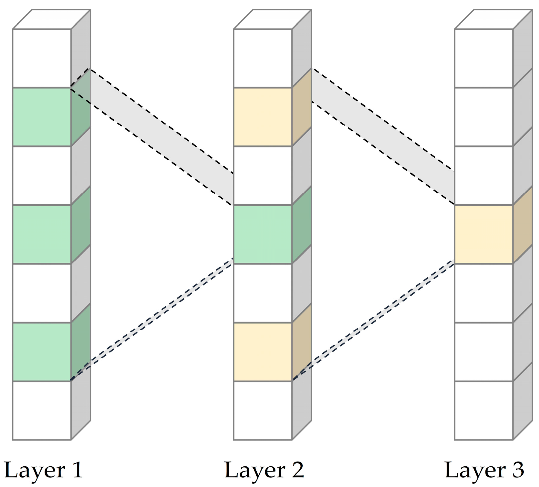
Residual connections, commonly known as shortcut or skip connections, as illustrated in Figure 7, play a pivotal role in addressing the challenges of vanishing or exploding gradients in deep neural networks [24]. These connections create shortcuts in the network architecture, allowing each layer to directly access the outputs of previous layers. This architecture facilitates the direct propagation of gradients during training, maintaining their strength across layers, and thus significantly improving the efficiency of the training process.

By enabling this direct flow of gradients, residual connections empower deep neural networks to more effectively process complex data patterns. This capability is particularly crucial for achieving deeper and broader learning within the network. The incorporation of these connections in deep networks ensures that even as the network depth increases, the learning process remains robust and effective, overcoming the common pitfalls associated with deep learning architectures.

4.2.2. Parametric Rectified Linear Unit

The integration of the PReLU as the activation function marks a critical enhancement in our CNN architecture [25]. PReLU represents an evolution of the traditional ReLU activation function, retaining its benefits such as non-linearity and computational efficiency while overcoming a significant limitation known as the ‘dying ReLU problem’, where neurons become inactive and output only zero. PReLU addresses this by introducing a small, learnable coefficient ($w$) for negative input values, shown in Equation (3).

$$f\left(x\right)=\left\{\begin{array}{cc}x& x>0\\ wx& x\le 0\end{array}\right.$$

(3)

where $x$ represents the input to a neuron, and $f\left(x\right)$ is the output after activation. The parameter $w$ is a small, learnable coefficient that provides a non-zero gradient for negative input values, thereby allowing for a small, controlled flow of the gradient during the backpropagation process. This coefficient $w$ allows for a controlled flow of the gradient during backpropagation, mitigating the gradient vanishing problem and enhancing the network’s ability to learn complex patterns.

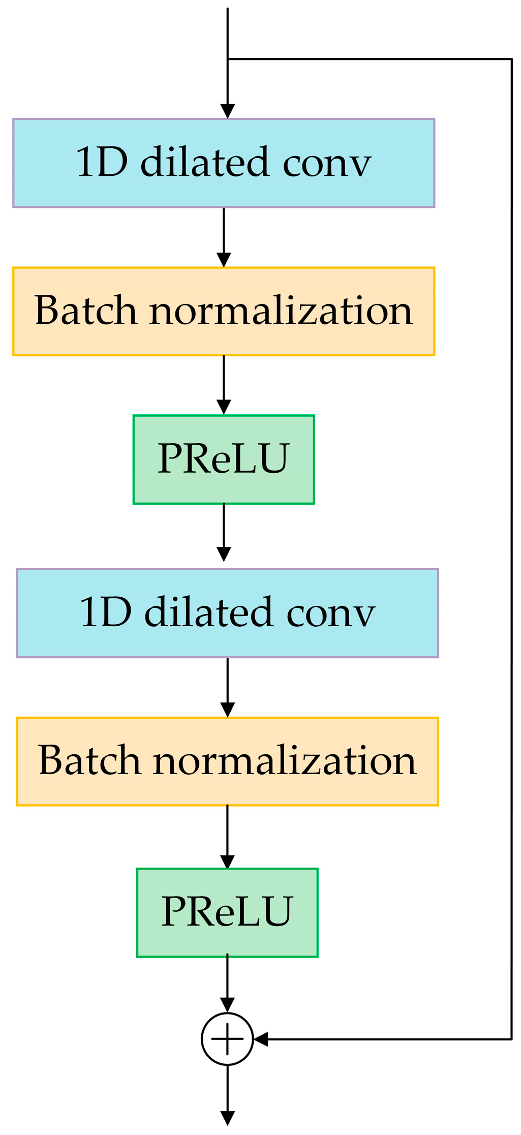
4.3. Innovations in Neural Network Architecture: The DRN Module

The DRN module in our neural network architecture, present in Figure 8, marks a significant advancement by synergistically integrating dilated convolutions, batch normalization, residual connections, and the PReLU. This innovative module combines the broadened receptive field offered by dilated convolutions with the gradient-enhancing capabilities of residual connections, along with the stabilizing influence of BN and the dynamic adaptability of PReLU.

Dilated convolutions in the DRN module expand the network’s field of perception without increasing computational costs, crucial for intricate spatial pattern recognition. This expansion allows the network to process extensive contextual information from input data more effectively. Residual connections within the module facilitate an unimpeded flow of gradients, addressing the common issue of gradient dissipation in deep neural networks. This feature not only promotes efficient training but also ensures that deeper network layers can learn identity functions, thus matching or surpassing the performance of shallower layers.

The integration of BN standardizes inputs across layers, achieving a uniform distribution that expedites training and enhances model generalization. Complementing this, the adoption of the PReLU activation function introduces a learnable parameter for negative input values. This parameter allows for a controlled flow of the gradient during backpropagation, enriching the network’s capacity to assimilate complex patterns and mitigating the limitations of standard non-linearity.

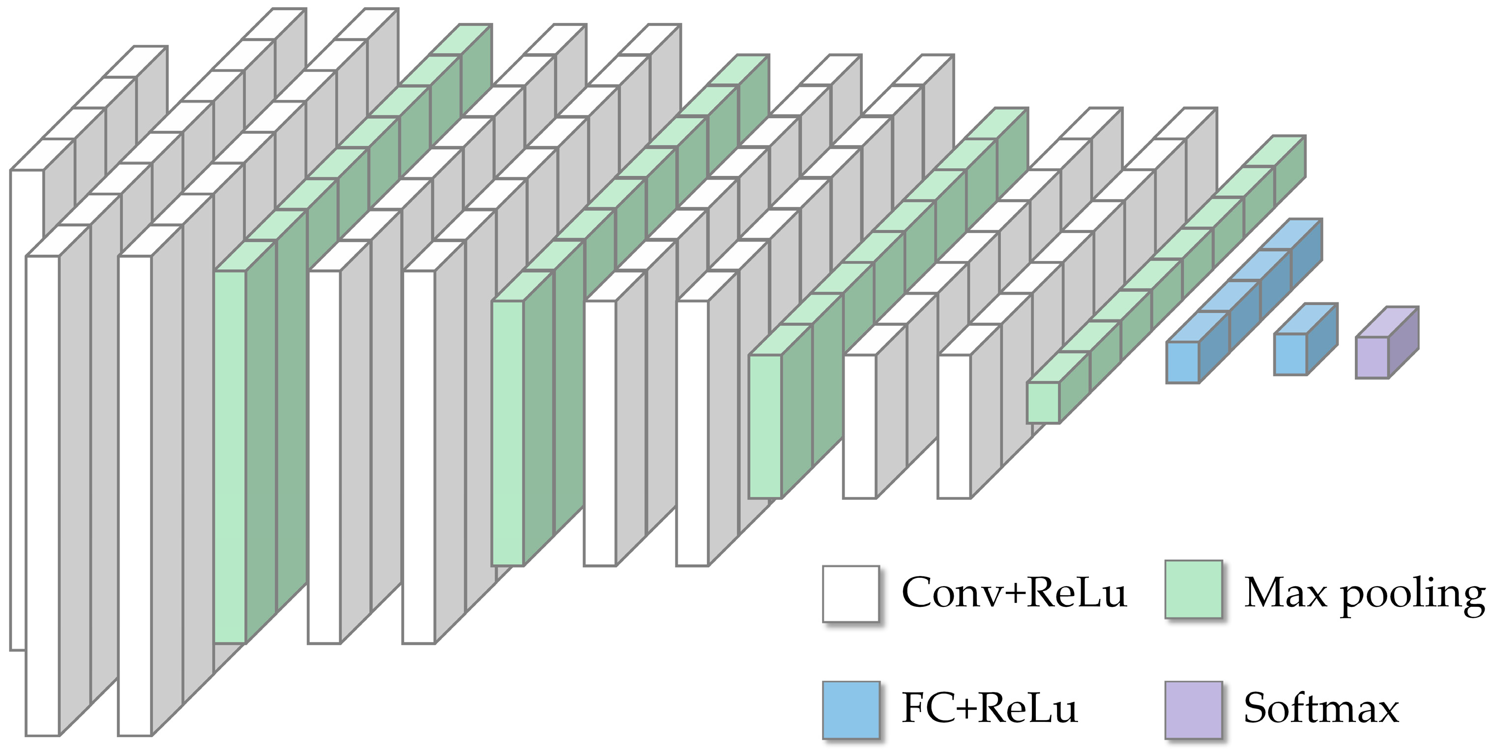
As depicted in Figure 9, the basic CNN model serves as the foundational framework upon which the DRN enhancements are superimposed. Building on this base, Figure 10 showcases the DRNCNN model, incorporating the DRN module into the traditional CNN architecture. This integration introduces advanced functionalities that address some of the inherent limitations of standard CNNs. The DRNCNN model, through the inclusion of the DRN Module, demonstrates how combining multiple technological advancements can improve the network’s ability to process and analyze complex datasets. It offers improved accuracy and efficiency for various computational tasks, illustrating the practical benefits of these enhancements in neural network design.

5. Case Study

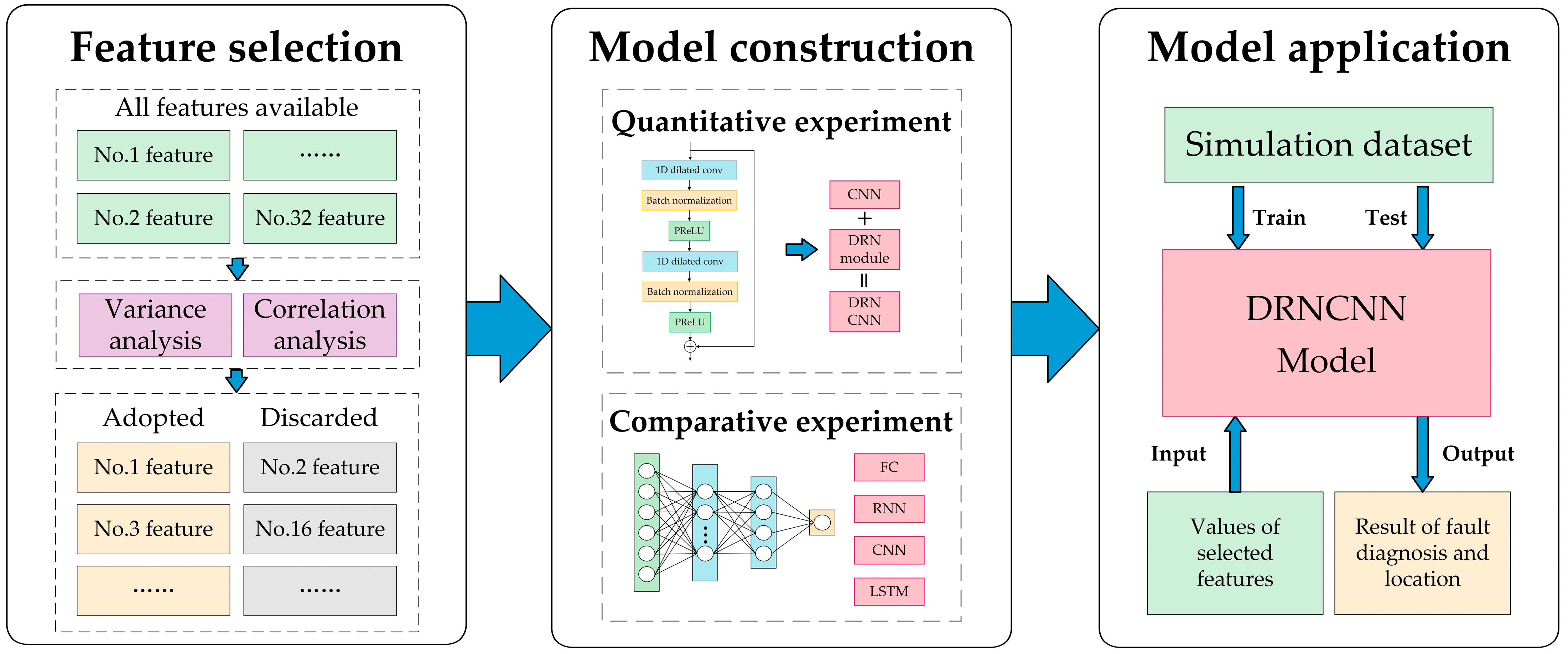
5.1. Data Processing

This research initiates with an extensive variance and correlation examination of the dataset, discarding features deemed irrelevant or superfluous to distill a core set of significant attributes, as depicted in Figure 11. The study then methodically processes fault data from DC filters to prepare for subsequent analysis. Initially focusing on a CNN as the foundational model, enhancements are applied through the incorporation of dilated convolution techniques, batch normalization, and PReLU, leading to the development of the advanced DRNCNN model. This model is evaluated against a simulation dataset, undergoing a comprehensive training and testing regimen to affirm its performance. Inputs to the DRNCNN model consist of selected feature values, which result in outputs that accurately delineate fault diagnostics and localization within the DC filters. This refined CNN model sets the benchmark against which other models, such as fully connected (FC) networks and Long Short-Term Memory (LSTM) networks, are subsequently compared to underscore its relative proficiency.

5.1.1. Variance Analysis

The first step of data processing is to perform variance analysis to assess the variability of each feature. During this process, features such as ‘IZ1T12rms’, ‘SER2DCP1’, ‘SER1DCP2’, ‘SER2DCP2’, ‘SER3DCP2’, ‘SER2DCP3’, and ‘SER1DCP4’ are identified to have zero variance, indicating that they are constant throughout the dataset and do not provide valuable information for the model. Therefore, to enhance model efficiency and reduce computational load, these features are removed from the dataset.

5.1.2. Correlation Analysis

The remaining features undergo correlation analysis to identify and remove highly correlated feature pairs. This analysis is conducted using Pearson correlation coefficient, whose formula is displayed in Equation (4).

$$r_{uv}=\frac{\sum _{i=1}^n(u_i-E(u\left)\right)(v_i-E(v\left)\right)}{\sqrt{\sum _{i=1}^n{\left(u_i-E\left(u\right)\right)}^2{\left(v-E\left(v\right)\right)}^2}}$$

(4)

where $r_{uv}$ represents the correlation coefficient, which quantifies the linear relationship between the variables u and v. The term n refers to the total number of data. Each data pair consists of corresponding sample points, denoted by $u_i$ and $v_i$, where i is the index of the sample points. The symbol $E\left(u\right)$ signifies the expected value, of the sample set for u, and similarly, $E\left(v\right)$ represents the mean of the sample set for v.

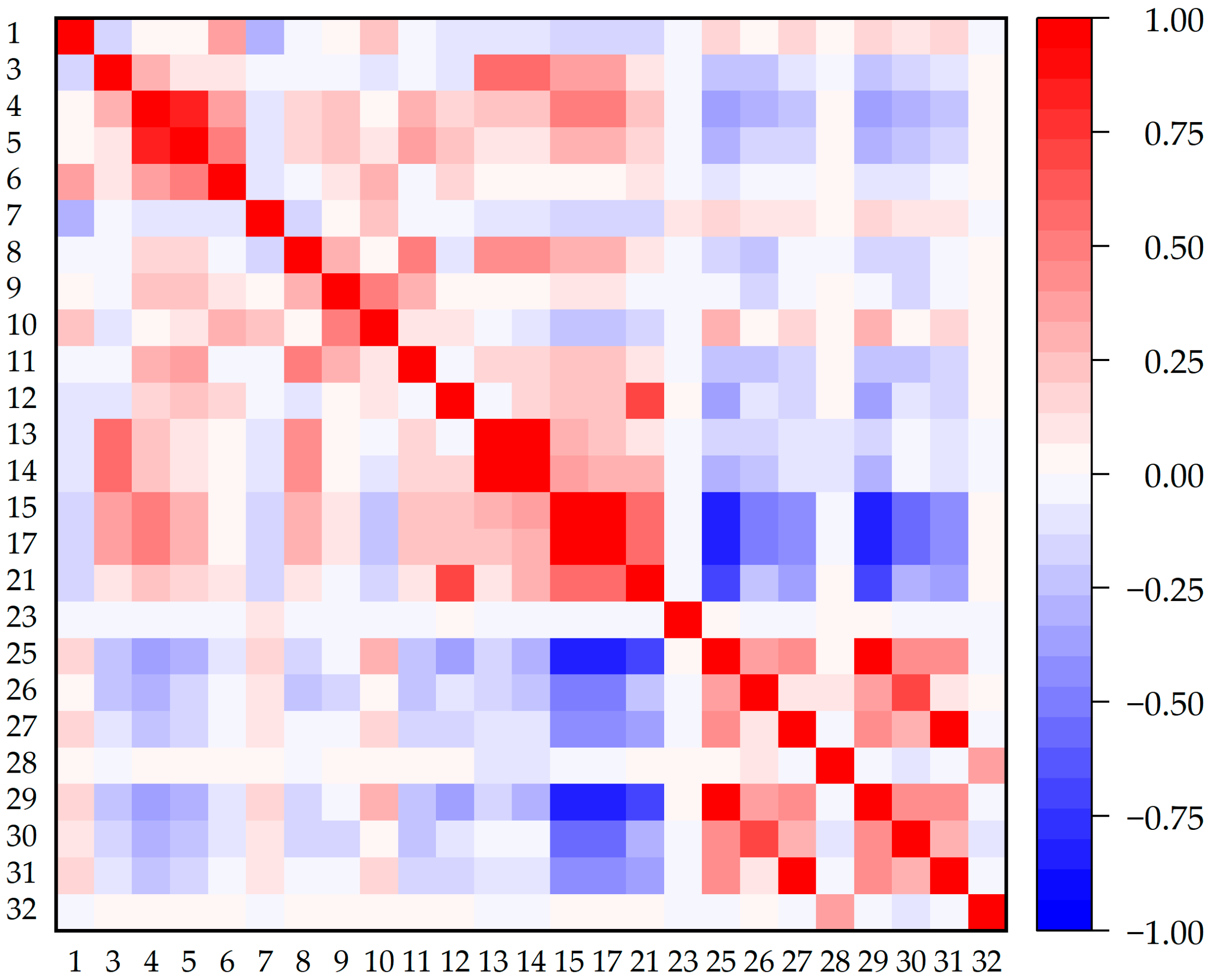
As depicted in Figure 12, the correlation analysis outcomes are effectively visualized using a correlation matrix plot. This plot succinctly illustrates the correlation levels among various features. In accordance with the analysis, if the correlation coefficient between any pair of features surpasses 0.9, such pairs are considered to exhibit high redundancy. Consequently, to mitigate multicollinearity within the feature set, one feature from each pair exhibiting high redundancy is omitted from the dataset. These pairs are systematically enumerated in

Table 3. Feature pairs with high similarity.

Feature Pair	Feature 1	Feature 2	Correlation Coefficient
1	Rectifier Station Pole 2 DC Line Current (28)	Inverter Station Pole 2 DC Line Current (32)	0.999916
2	Rectifier Station Pole 2 DC Line Voltage (26)	Inverter Station Pole 2 DC Line Voltage (29)	0.996388
3	SER2DCP1 (16)	SER1DCP2 (18)	0.989927
4	DC Filter Differential Current (14)	SER1DCP1 (15)	0.976978

.

5.1.3. Normalization

To eliminate the impact of different scales among features, it is necessary to normalize the data to ensure comparability. The min–max normalization method is used to scale the data, bringing feature values into the [0,1] range, as shown in Equation (5).

$$D_{norm}=\frac{D-D_{min}}{D_{max}-D_{min}}$$

(5)

where $D$ is the original value, $D_{min}$ is the minimum value of the feature, and $D_{max}$ is the maximum value of the feature. This process ensures that all features contribute equally to the model, improving its ability to learn from the data effectively.

5.1.4. Dataset Division

To eliminate the influence of transient characteristics at the initial stage of the fault and to enhance data utilization, the dataset is first divided into a training set and a test set in an 8:2 ratio. Following this division, within each subset, a 0.5 s segment of data is randomly selected five times from the simulation time between 2.1 and 4.1 s for each operating state. This process, applied separately to both the training and test sets, ensures that each sample contains 1000 data points. By adopting this methodology, the study provides a comprehensive and diversified dataset by capturing multiple snapshots of the same operational state through varied sampling instances, allowing for effective evaluation of the proposed model’s performance on independent data.

5.1.5. Performance Metrics in Fault Diagnosis

In the realm of fault diagnosis, four primary performance metrics are crucial [26]: accuracy, precision, recall, and F1 score. These metrics are instrumental in evaluating the efficacy of fault diagnosis models. Considering the presence of 27 distinct classes in the scenario, it becomes essential to compute these metrics individually for each class and subsequently derive their average values across all classes. For each class, data identified as belonging to that class are deemed positive. This positive classification is further delineated into true positives (TP) and false positives (FP). TP refers to the number of data points correctly identified as belonging to the class, whereas FP denotes those data points incorrectly classified as belonging to it. In contrast, data not associated with this class are labeled as negative. This category is further split into true negatives (TN) and false negatives (FN). TN represents data points accurately identified as not belonging to the class, while FN includes those incorrectly marked as not belonging to the class. The counts of TP, FP, TN, and FN for each class are pivotal for computing the aforementioned metrics. The formulas for calculating accuracy (acc), precision (pre), recall (rec), and F1 score are shown as Equations (6) to (9).

$$pre=\frac{TP}{TP+FP}$$

(6)

$$rec=\frac{TP}{TP+FP}$$

(7)

$$F1=\frac{2\times pre\times rec}{pre+rec}$$

(8)

$$acc=\frac{TP+TN}{TP+FP+TN+FN}$$

(9)

These formulas provide a comprehensive assessment of the model’s performance in accurately classifying each class, taking into account both the correct and incorrect classifications.

5.2. Case 1: Evaluation for the Improved CNN Model

In this case study, we present an improved CNN architecture that incorporates a DRN module to enhance model performance. This DRN module is a fusion of four advanced elements: residual connections (A), BN (B), dilated convolutions (C), and PReLU (D). We undertake an ablation study for our experimental design, methodically evaluating the contribution of each technique to the model’s effectiveness by sequentially integrating them. The initial architecture is shown in Figure 9, which forms the basis for our incremental enhancements, culminating in the ultimate architecture with all four modules combined, as depicted in Figure 10.

As is shown in

Table 4. Performance metrics of the improved CNN.

Model	Acc (%)	Pre	Rec	F1
CNN	89.316	0.9096	0.8931	0.8870
CNN + A	91.310	0.9402	0.9131	0.9111
CNN + B	92.877	0.9473	0.9287	0.9311
CNN + C	90.743	0.9190	0.9074	0.9087
CNN + D	92.450	0.9440	0.9245	0.9232
CNN + A + B	98.148	0.9834	0.9814	0.9815
CNN + A + C	96.438	0.9721	0.9643	0.9652
CNN + A + D	96.011	0.9642	0.9601	0.9604
CNN + B + C	97.863	0.9822	0.9786	0.9790
CNN + B + D	96.581	0.9704	0.9658	0.9664
CNN + C + D	96.296	0.9683	0.9629	0.9630
CNN + A + B + C	99.002	0.9916	0.9900	0.9900
CNN + A + B + D	98.860	0.9905	0.9886	0.9886
CNN + A + C + D	96.011	0.9698	0.9601	0.9606
CNN + B + C + D	98.005	0.9834	0.9800	0.9803
CNN + A + B + C + D	99.287	0.9943	0.9928	0.9929

Note: In the first column, “A”, “B”, “C” and ”D” represent residual connections, BN, dilated convolutions and PReLU, respectively.

, the experimental results begin with evaluating the performance of the baseline CNN model, followed by the step-by-step addition of the improved components. We observed that each new component added led to an enhancement in the model’s accuracy (Acc), precision (Pre), recall (Rec), and F1 score. With the integration of all improvement components A, B, C, and D into the CNN, the model demonstrated the best performance, achieving an accuracy of 99.287% and an F1 score of 0.9929. These significant results underscore the efficacy of the DRN module in enhancing CNN models.

Upon reviewing the experimental data, it is evident that each technological enhancement significantly improved the model’s performance. Dilated convolutions (B), by expanding the receptive field, notably increased accuracy, as seen in models like CNN + B (92.877% accuracy) and CNN + A + B (98.148%). Residual connections (A) effectively addressed the vanishing gradient problem in deep networks, evident from the improved results in models like CNN + A (91.310%) and CNN + A + B. Batch normalization (BN) accelerated training and improved stability, demonstrated by models like CNN + B (92.877%) and CNN + A + B. This improvement is clearly illustrated in Figure A1. The use of PReLU (D) also enhanced performance, as observed in models like CNN + D (92.450%) and CNN + A + D (96.011%).

The combined use of these technologies resulted in even more significant improvements. Models incorporating multiple enhancements, such as CNN + A + B + C + D, achieved the highest accuracy of 99.287%. This synergy highlights the effectiveness of integrating various advanced techniques in model development.

In addition to the aforementioned improvements, the incorporation of t-distributed stochastic neighbor embedding (t-SNE) visualization substantiates the effectiveness of our final model’s feature extraction capabilities. As is shown in Figure 13, by presenting a clear delineation of class clusters in a reduced dimensional space, t-SNE affirms the model’s enhanced discriminative capacity, enabling a more intuitive understanding of its classification boundaries and the high-quality feature representations it has learned. We apply t-SNE to the feature representations learned by our final model to project them into a two-dimensional space. This projection allows us to observe the clustering of different classes and to understand how well the model separates distinct categories in the feature space. The visualization provides an intuitive illustration of the model’s ability to discern and categorize various data points, highlighting the distinct clusters formed by different classes. Such a representation is instrumental in assessing the quality of the learned features and the model’s overall discriminative power.

Following t-SNE visualization, the construction of a confusion matrix provided a quantitative validation of the model’s discriminative prowess, complementing the t-SNE analysis and confirming the robustness and precision of the class predictions [27,28]. Within this matrix, the rows represent the actual class instances, and the columns signify the predicted class instances by the model. Correct classifications are depicted along the diagonal, where the predicted labels match the true labels, evidencing the model’s strong predictive performance. This matrix elucidates the model’s overall classification effectiveness, clearly indicating a high rate of accuracy in predictions and underscoring the model’s competency in fault diagnosis. The successful application of the model on test samples and the corresponding high-quality classification outcomes are encapsulated in Figure 14.

5.3. Case 2: Comparative Experiment

In the case study section of the paper, a series of comparative experiments were conducted to evaluate the performance of the enhanced model. The DRNCNN, embodying the latest advancements in neural network architecture, was juxtaposed against traditional architectures, including fully connected (FC) networks, Recurrent Neural Networks (RNNs), and Long Short-Term Memory (LSTM) networks [10]. These comparative trials aimed to underscore the efficacy of the DRNCNN model in handling complex datasets, specifically those associated with fault detection in DC filters. Metrics for comparison encompassed a range of performance indicators such as accuracy, precision, recall, and F1 score, ensuring a comprehensive assessment of each model’s capabilities in the context of fault diagnosis and localization. As is shown in

Table 5. Performance metrics of base neural network models.

Model	Acc (%)	Pre	Rec	F1
FC	85.312	0.8674	0.8631	0.8606
RNN	90.028	0.90.08	0.9002	0.8869
Basic CNN	89.316	0.9096	0.8931	0.8870
LSTM	95.293	0.9582	0.9529	0.9530
DRNCNN	99.287	0.9943	0.9928	0.9929

and Figure 15, the results of these experiments are integral in demonstrating the superiority of the DRNCNN model over conventional approaches, highlighting its potential to revolutionize predictive maintenance in power systems.

The experimental data leads to several key insights about the performance of different neural network architectures. Contrary to the initial analysis, it is evident that while CNNs (basic CNN with 89.316% accuracy) are effective for local feature extraction from sequential data, they are not the top-performing model in this comparison. The CNN’s strength lies in its ability to identify crucial characteristics within time series, especially in contexts like direct current filter fault data where localized temporal correlations are significant.

Contrary to emerging as a strong contender, FC networks actually displayed the weakest performance among the models tested, with an accuracy of 85.312%. Their simplicity and ease of training do not compensate for their limitations in handling high-dimensional data analysis. With an extensive parameter set yet restricted feature extraction capabilities compared to more advanced architectures like CNNs, FC networks struggle to effectively identify complex patterns in time series data. This inherent drawback positions them as the least effective model in this experimental comparison.

RNN (90.028% accuracy) and LSTM (95.293% accuracy) showed mixed results. While known for handling long-term dependencies, these architectures did not perform as well in this specific dataset, possibly due to the dataset’s characteristics or the computational complexity of RNN and LSTM, which could lead to longer training and prediction times.

The DRNCNN model, boasting an exceptional accuracy of 99.287%, clearly outperforms other models in this comparison. This enhanced variant of a standard CNN incorporates dilated convolutions to widen the receptive field and includes residual connections to effectively address the vanishing gradient problem. Moreover, the integration of batch normalization (BN) and parametric rectified linear unit (PReLU) activations significantly contributes to stabilizing and optimizing the learning process.

It is worth noting that, as shown in Figure 15b and Figure A1p, DRNCNN exhibits a faster iteration speed and enhanced stability compared to traditional CNN. These advantages, in addition to its remarkable accuracy, unequivocally establish the superiority of the DRNCNN model in this experimental evaluation.

6. Conclusions

This paper has established a novel CNN methodology for the fault diagnosis in DC filters. By conducting a thorough variance and correlation analysis to remove invalid and redundant data, the study has formulated a deep neural network with a strategically optimized structure. This network, encompassing four convolutional layers and two fully connected layers, leverages a streamlined set of features to enhance precision and reduce the risk of overfitting, achieving an impressive fault identification accuracy of 99.28% across various power levels and wiring methods.

The crux of the innovation presented in this paper is the development of the DRNCNN model. The DRNCNN model, which integrates dilated convolutions, residual connections, BN, and the PReLU, not only builds upon the inherent strengths of traditional CNNs but also ameliorates their limitations by enhancing gradient flow and broadening the receptive field without incurring extra computational costs. The robustness of the DRNCNN against vanishing gradients and its superior generalization capabilities have been demonstrated to be exceptionally effective for quick and precise ground fault identification in DC filters.

This research provides a comprehensive and efficient technical roadmap for fault localization in HVDC system direct current filters, addressing the challenge of overfitting typical of CNN models and enhancing computational efficiency and practical applicability. The conclusive findings of this study not only affirm the efficacy of the DRNCNN model in fault diagnosis but also highlight its potential to serve as a pivotal innovation in the predictive maintenance of power systems. This work lays the groundwork for future research, promising significant contributions to the reliability and efficiency of neural network-based diagnostic tools in power systems.