An Internet-of-Things-Based Dynamic Scheduling Optimization Method for Unreliable Flexible Manufacturing Systems under Complex Operational Conditions

Abstract

The dynamic scheduling problem (DSP) in unreliable flexible manufacturing systems (UFMSs) with concurrency, conflicts, resource sharing, and sequential operations is a complex optimization problem that requires the use of efficient solution methodologies. The effectiveness of scheduling UFMSs relies on the quality of equipment maintenance. Currently, UFMSs with consistently large queues of parts awaiting service employ a repair-after-failure approach as a standard maintenance procedure. This method may require unexpected resources, incur costs, consume time, and potentially disrupt the operations of other UFMSs, either partially or fully. This study suggests using a predictive maintenance (PdM) strategy that utilizes the Internet of Things (IoT) to predict and avoid early mechanical equipment failures before they happen in UFMSs, thereby reducing unplanned downtime and enhancing reliability. Therefore, the objective of this paper is to construct timed Petri net (TPN) models using the IoT for the PdM configuration of mechanical equipment in the dynamic scheduling problem of UFMSs. This necessitates that users represent the specific problem using TPNs. The process of PN modeling requires the utilization of domain knowledge pertaining to the target problems as well as to machine information. However, it is important to note that the modeling rules for PNs are straightforward and limited in number. Consequently, the TPN model is applied to generate and formulate mixed-integer linear programming (MILP) instances accurately. This is done to identify the optimal production cycle time, which may be implemented in real-life scenarios. Several UFMS instances are used to demonstrate the applications and effectiveness of the proposed method. The computational results demonstrate that the proposed method shows superior solution quality, effectively solves instances for a total of 10 parts and 6 machines, and achieves a solution in a reasonable CPU time.

1. Introduction

Flexible manufacturing systems (FMSs) are computer-controlled systems that can automatically execute a variety of activities based on predetermined process plans. The FMS includes a restricted number of resources, including machines, robots, automated guided vehicles (AGVs), and buffers, which are shared by multiple production processes within the system [1]. In an FMS, raw components are simultaneously processed in a predefined sequence to efficiently use constrained system resources and enhance overall system performance [2].

There are two major issues involved with the operation of an FMS: structural (design) issues and operational issues. The number of machine tools of each kind, the size of the material handling system, and the capacity of the buffers are FMS design considerations. FMS operational issues involve problems with planning, scheduling, and control. The decision of which parts should be sequentially machined and the assignment of pallets and fixtures to part kinds are planning issues. Given the selected part mix, the FMS scheduling problem involves deciding the optimal input order for components and the optimal order at each machine. The FMS control problems include observing the system to ensure that requirements and deadlines are met as well as addressing deadlock problems [3]. Real-world FMSs can be subject to unexpected uncertainties, including operator errors, machine malfunctions, and uncertain part processing times. Subsequently, the FMS encounters difficulties dealing with modifications in the manufacturing plans or orders. Hence, in order to enhance the promptness and adaptability of FMSs in dealing with uncertainties, it is imperative to optimize production scheduling, which is referred to as the dynamic scheduling problem (DSP). This entails adjusting the production scheduling strategies of FMSs based on the current production status in order to effectively adapt to the dynamic environment. Several combinatorial optimization problems (COPs) are NP-hard, and no solutions to these problems have been presented [4]. In the fields of manufacturing, agriculture, transportation, medical services, and sciences, combinatorial optimization can be used to minimize costs or maximize the impact of different systems. Optimization plays a crucial role in obtaining sustainable development objectives [5,6]. The era of big data has increased the significance of optimization studies, which extract important information from data using optimization methods [7,8,9]. Thus, this study has been considered one of the most significant subjects. If the feasible area is bounded, “integer programming” (IP) can be used to formulate combinatorial optimization problems [10]. This method is known as “integer linear programming” (ILP) if the objective function and all constraints of the COP are stated as linear equations. By combining integer and real variables in the mixed formulation, a greater number of COPs can be generated in comparison with simple IPs [11]; this is known as “mixed-integer programming” (MIP). When only linear constraints and objective functions are involved, therefore, MIP problems are referred to as “mixed-integer linear programming” (MILP) problems [12]. The FMS scheduling problem is a complicated optimization problem that is defined as NP-hard [13,14,15,16]. It is not feasible to find an exact solution to an FMS scheduling problem within an acceptable amount of time, even for instances of small size [16]. The optimal solution necessitates an exponential time frame. Hence, the solution to this NP-hard problem needs the utilization of metaheuristic methods. Researchers in the field of FMS scheduling have proposed several metaheuristic approaches, including the genetic algorithm (GA) [14,15,16,17,18], the ant colony optimization algorithm (ACO) [18,19], particle swarm optimization (PSO) [18,20], simulated annealing (SA) [21,22], Tabu Search (TS) [23,24], etc.

At present, simulation software is widely used for scheduling in several industries to guarantee the effective running of manufacturing processes, both technically and economically. Gholami and Zandieh [25] integrate the simulation and the genetic algorithm to minimize makespan and mean tardiness in flexible job-shop scheduling with machine stochastic breakdowns. Pergher et al. [26] combine simulation with the flexible and interactive tradeoff compensatory approach in job-shop production systems to determine the best combination of due order release, date assignment, and shop dispatching rules. Different combinations are assessed based on production quantity, total cost, total throughput time, and tardiness. Thenarasu et al. [27] integrate the simulation and the multi-criteria decision-making approaches to the model and evaluate flow time, makespan, and tardiness-based measures in partial flexible job-shop scheduling with both static and dynamic job arrivals. The open-source program Lekin is used to analyze and simulate the impact of dispatching rules on the makespan time in the flexible job-shop system [28]. The software also identifies the most efficient manufacturing process layout that minimizes production time [29].

Petri nets (PNs) are effective modeling and simulation tools for LP, ILP, and MILP problems because PNs contain mathematical expressions indicated as linear equations [30,31]. The work in [32] presented a method for constructing MILP based on PN models for combinatorial optimization problems involving “traveling salesman problems” and a “simple resource assignment problem”. Tuncel and Bayhan [33] provided a comprehensive study of scheduling challenges in which they highlighted the integration of Petri nets with other approaches and addressed both theoretical developments and practical experiences. Existing approaches have been divided into four categories: (1) Petri net-based simulations connected with “heuristic dispatching rules” for the control and scheduling of manufacturing systems; (2) generative scheduling methods in which Petri nets are applied to develop schedules in terms of the transition firing sequences through the “reachability graph”; (3) a special Petri net class model employed to construct the planning and scheduling problem as a mathematical model; and (4) Petri net modeling approach providing a basis for the search procedure of metaheuristic methods to find the near-optimal “resource allocation” and the “event-driven schedule” in terms of the Petri net model firing sequences of the transitions. Wu et al. [34,35] constructed a Petri net model to represent wafer production processes in cluster tools requiring wafer revisitation. They proposed a systematic approach for evaluating their effectiveness, which leads to the derivation of optimality requirements for three-wafer period scheduling. Qiao et al. [36,37] constructed a model to represent wafer production processes using a “timed Petri net” to optimize their schedule. Analytical expressions can be used to determine whether the systems are schedulable. They also provided a simple implementation method for the obtained schedule. Using PNs, Zhou et al. [38] modeled and evaluated an FMS cell. They used “top-down refinement”, “system decomposition”, and “modular composition ideas” to obtain the structure and preservation of essential system characteristics, such as “liveness”, “boundedness/safety”, and “reversibility”, which ensure the system’s “stability”, “deadlock-free”, and “cyclic manner”. A reduction approach was applied to transform the timed PN to an equivalent time-marked graph. Then, the typical method for determining cycle time for the marked graphs was implemented. In addition, Zhou et al. [39] developed PN models for FMS by scheduling the modeled FMS based on the firing sequences of the PN model from the initial marking to the final one. Using a class of timed PNs, they applied a branch-and-bound approach to determine the optimal schedule for the FMS. Artigues and Roubellat [40] proposed a PN model in the context of a generic approach for “on-line” scheduling in a job shop environment with various setup times and resources based on a detailed definition of essential states, decisions, and events for “on-line” and “off-line” scheduling. They used an “acyclic directed graph” to illustrate a set of static scheduling problem solutions. Mejia and Odrey [41] introduced Beam A* Search, a PN-based algorithm (BAS). This approach systematically increases segments of a PN “reachability graph” in order to identify a schedule that is close to optimal. Their proposed technique was evaluated by applying it on various FMS scheduling problems. Zhang et al. [42] modeled the assembly processes of the “flexible assembly system” using timed Petri nets (TPNs). A scheduling model was developed for the FAS, and a dynamic programming method was used to determine a viable allocation of processes to machines and to optimize the time to completion for either a “single product” or a “batch of products”. In their study, Kim et al. [43] introduced a new scheduling approach for production systems that relies on the TPN model and a “reactive fast graph search” approach. The main objectives of this method are to minimize the maximum completion time (makespan) and the overall tardiness. In order to accomplish the objectives, they proposed a new search algorithm that integrates the “RTA*” with a “rule-based supervisor”. Lee and Lee [44] developed heuristic functions for the A* method based on T-timed PNs for the purpose of optimizing the FMS scheduling problem by reducing the makespan. In addition, they developed enhanced versions of these heuristic functions, which obtained an initial near-optimal solution faster. Wang and Wang [45] investigated the FMS scheduling problem based on a PN with the objective of minimizing the makespan. Combining a “dynamic search window” with a “best-first algorithm” and “backtracking search”, they proposed a hybrid heuristic search method for the scheduling problem. Kammoun et al. [46] developed a mathematical model that uses the properties of decomposed TPNs to address the FMS scheduling problem. The model aims to determine the optimal firing sequence of TPN transitions and minimize the total processing time. Moreover, a genetic algorithm was presented to find effective solutions for large-scale scheduling problems. With the objective of finding an optimal transition sequence that minimizes firing time, the authors of [47] proposed a new “admissible heuristic function” for scheduling FMSs utilizing P-timed PNs. Using the structural symmetry of a PN model of an FMS to make a partial reachability graph reduces the state explosion problem as much as possible. The estimate function is applied to each generated marking to calculate the cost of firing the transition sequence. PNs’ ability to describe multiple states concisely, capture priority relations and structural connections, and model “deadlocks”, “conflicts”, “buffer sizes”, and “multi-resource constraints” are the primary advantages of implementing PNs in the FMS scheduling issue compared with alternative approaches. This will assist system analysts in modeling complicated, integrated scheduling issues [45]. Most researchers who studied the scheduling problem in industrial systems used the “reachability tree”. It is well known that the size of a “reachability tree” increases exponentially as the size of a PN increases. This makes it rather challenging to evaluate PN models with a significant number of places and transitions.

Several organizations are depending on a single maintenance approach to guarantee the optimal efficiency of their resources. Regrettably, only a small number of individuals take into account the expenses incurred by ignoring the monitoring of asset deterioration during the early phases of defect formation. Maintenance can be categorized into three distinct types: corrective maintenance (CM), preventive maintenance (PM), and predictive maintenance (PdM). PM and CM primarily revolve around the age of the asset and adhering to a regular maintenance schedule. However, their drawback lies in the fact that they address resource repairs only when they have reached an advanced degree of deterioration. Frequently, these resources experience failures during the intervals between inspections, resulting in escalated repair expenses and significant hazards to human safety. Many companies mistakenly believe that a strategy that combines breakdown maintenance and the life of the resource is enough to accurately anticipate resource failure. Frequently, they neglect significant faults that result in severe malfunction and necessitate the replacement of resources rather than their repair, resulting in additional expenses. During CM, maintenance workers promptly commence work upon the occurrence of a problem. The objective of CM is to expedite the restoration of systems to their normal functioning state. CM does not involve a scheduled program for normal maintenance. Maintenance can take place only when there is an existing problem. The cost of repairs may be marginally higher, but it is significantly more affordable than the expense of routinely employing staff to maintain equipment. The equipment is repaired promptly; however, this approach can have adverse consequences in the event of a catastrophic occurrence. PdM is an improved approach to performing maintenance activities. It involves using test results and trends to anticipate or identify issues with a component of equipment. These methods employ noninvasive testing procedures to quantify and calculate trends in equipment performance. Some examples include vibration analysis, infrared analysis, thermography, ultrasound, and various other techniques.

The IoT enables the connection of physical things, enabling them to communicate information via the Internet. This capability has the potential to facilitate the collection of large volumes of data, which may be a strong asset for the success of businesses and future predictions [48,49]. At present in the field of maintenance, the use of embedded hardware consisting of sensors and other intelligent equipment controlled by the IoT is changing industrial and manufacturing operations [50,51]. The utilization of IoT in the predictive maintenance approach can be highly effective in this context. It involves directly monitoring equipment by continuously capturing real-time data on key stress-related variables, such as noise level, temperature, vibration, pressure, power consumption, and other interconnected devices [52]. This allows users to gain visibility into the performance of their assets and discover valuable insights. It also enables the detection of anomalies, the identification of patterns, and the recognition of warning signals that may indicate an imminent failure [52,53].

As mentioned in the literature, repairing UFMS equipment is a standard procedure because the equipment often fails without any prior communication to the maintenance team. As a result, the detection of faults and the subsequent unplanned maintenance can disrupt the current operations of the remaining UFMSs, either fully or partially. In order to enhance the use, availability, and reliability of equipment and minimize the costs associated with equipment maintenance, it is crucial for the maintenance team to have access to real-time condition-based data. This allows for efficient repairs and minimizes downtime, unnecessary inspections, maintenance time, and undue pressure on the maintenance team [54,55]. Motivated by the issues mentioned previously, this study identifies a lack of adoption of current PdM systems for this type of equipment. This is caused by variations in mechanical characteristics among various equipment and the absence of historical or real-time performance data. Therefore, the main contribution of this paper is to develop TPN models for the dynamic scheduling problem of UFMSs with concurrency, conflicts, resource sharing, and sequential operations. Subsequently, the proposed TPN model is utilized to generate the MILP in order to determine the optimal production cycle time, which can be implemented in real-life situations. Additionally, the paper proposes the utilization of the IoT for the PdM configuration to prevent early mechanical equipment malfunctions in UFMSs and avoid interruptions in the scheduled operations of other UFMSs. Finally, several cases of UFMSs are used to demonstrate the practical applications and effectiveness of the proposed approach.

The rest of the paper is organized as follows: Section 2 introduces timed Petri net synthesis and the estimation of resource failure time using the Internet of Things. Section 3 describes a statement and MILP model based on TPN to address the dynamic scheduling problem in unreliable flexible manufacturing systems with concurrency, conflicts, resource sharing, and sequential operations constraints. Section 4 demonstrates the practical use and effectiveness of the developed MILP model through the use of instances. Section 5 presents a brief summary and outlines the future research endeavors of the study.

2. Preliminaries

2.1. Timed Petri Nets Synthesis

Petri nets are a mathematical modeling tool that involves symbols such as place, transition, arc, and token, as depicted in Figure 1. The original PN did not indicate any time aspect. Timed Petri nets (TPNs) are created by including time in the PN to evaluate performance associated with time. TPNs are formally defined as a six-tuple N = (P, T, F, W, h(T), M) where:

• P = P_A ∪ P_R: represents a non-empty finite set of model places, where P_A = ∪_i∈|m|{p_i}, m > 0 and P_R = ∪_i∈k{p_mk}, k > 0 represent sets of model operation and resource places, respectively;
• T = ∪_j∈|T|{t_j}: represents a non-empty finite set of model transitions, P ∩ T = ∅, and P ∪ T ≠ ∅;
• F ⊆ (P × T) ∪ (T × P): represents flow relations and is denoted by arcs connecting places to transitions (P × T) or from transitions to places (T × P);
• W: (P × T) ∪ (T × P) → IN: is the weight-to-arc affectation function, where IN = {0, 1, 2, …}.
• h(t_j) ∈ h(T): denotes the static time that is assigned to t_j, t_j ∈ T;
• ^•p_i(p_i^•): represents the input transitions (and corresponding output) of the place p_i;
• ^•t_j(t_j^•): represents the input places (and corresponding output) of the transition t_j;
• M: P →IN denotes the function of the marking, which allocates to p_i ∈ P a number of tokens, the initial marking is denoted by M_o, and place marking is represented by M(p_i);
• M[t_j⟩: represents that at marking M, the transition t_j can be fired.

Figure 1. Icons for the Petri net symbols.

Figure 1. Icons for the Petri net symbols.

It is essential to note that marking M enables the transition t_j to be fired if M(p_i) ≥ W(p_i, t_j), t_j ∈ p_i^•. When the transition t_j ∈ T is enabled at marking M, the marking M can be modified from M to a new marking M′, designated as M[$t⟩$ M′ and expressed as follows:

$$M^{\prime }\left(p_i\right)=\left[\begin{array}{ll}M\left(p_i\right)+W\left(p_i, t_j\right)& \mathrm{if} p_i\in {}^{•}t_j\setminus {t_j}^{•}\\ M\left(p_i\right)-W\left(t_j,p_i\right)& \mathrm{if} p_i\in {t_j}^{•}\setminus {}^{•}t_j\\ M\left(p_i\right)+W\left(t_j, p_i\right)-W\left(p_i, t_j\right)& \mathrm{if} p_i\in {t_j}^{•}\cap {}^{•}t_j\\ M\left(p_i\right)& \mathrm{otherwise}\end{array}\right]$$

(1)

To represent the synthesis of the TPN model, consider Figure 2, which consists of three places and two transitions. The transition t₁ is enabled at the initial marking M_o = p₁ + 0p₂ + 0p₃, i.e., M_o[t₁⟩. At M_o, the transition t₁ fires after two time slices (t.s). It selects a token from p₁ and deposits one token into p₂. Then, it creates a new marking M₁ = 0p₁ + p₂+ 0p₃ and expresses it as M_o[t₁⟩ M₁. Similarly, at M₁, the transition t₂ is enabled and can be fired with a delay of 4 t.s to create a succeeding marking, which can be expressed as M₁[t₂⟩ M₂ with M₂ = p₁ + 0p₂ + p₃.

There are typically three types of places for PN models of FMSs: the set of idle places, the set of operation places, and the set of resource places. The number of tokens in the corresponding operation place at the initial marking indicates the maximum number of jobs that can be processed concurrently for a certain job type. In this study, an idle place is referred to as a sink place. The sink place is free of output transitions. A token at an initial operation place denotes a raw job that is ready for processing, while a token in a sink place indicates a finished job. In an FMS, resource places represent the resources (such as machines and robots). At the initial marking, the tokens in a resource place reflect the available resource units. The operation places, which are initially unmarked, represent the procedures that must be completed for the jobs in the production sequences. On the basis of timed PNs, each transition is associated with a time delay that indicates the time that is required to perform the appropriate operation. When the token’s time delay finishes, it becomes available at an operation place.

In order to demonstrate the modeling of TPNs, consider an FMS, presented in Figure 3, that is composed of two machines m = 1, 2, operating two different jobs i = 1, 2, in a sequential manner; one robot, r₁ (material-handling equipment); and a load/unload station.

Table 1. Scheduling data of an FMS shown in Figure 3.

Job	Operation	Time	Machine
1	1	4	1
	2	6	2
2	1	8	2
	2	10	1

displays the sequence of job-production operations, the duration of each operation, and the machine that can be used for each operation. As shown in Table 1, each job involves a set of operations. For instance, job 1 contains two operations that sequentially require m₁ and m₂. Thus, job 1 can be completed sequentially using machines m₁ and m₂ with corresponding processing times of 4 and 6, respectively.

Figure 4 illustrates the TPN model for this system, and the description of places and transitions in the TPN model is given in

Table 2. Description of places and transitions of the TPN model shown in Figure 4.

Places	Description
p11	Process 1 for part 1
p12	Process 2 for part 1
p21	Process 1 for part 2
p22	Process 2 for part 2
pm1	Machine 1 is available
pm2	Machine 2 is available
t11	End process 1 of part 1
t12	End process 2 of part 1
t21	End process 1 of part 2
t22	End process 2 of part 2

.

2.2. Estimation of Resource Failure Time Using IoT

In the context of FMSs, the term “resource failure” denotes an issue characterized by temporal uncertainty. In case of a “resource failure”, it is necessary to establish a “recovery subnet” with the ability to fix the problem [56]. The resource possesses the characteristic of reusability. This section aims to provide formal definitions for the purpose of estimating the occurrence of faults in an FMS using the IoT. It is assumed that the system contains sensors for the purpose of detecting the occurrence of resource breakdowns. The sensors facilitate the transmission of data to the Internet. Consequently, the gathered data can be accessed from any geographical point across the world. After the transmission of data to the Internet, a computer system will initiate the process of downloading and then utilize the acquired data to identify and rectify any cases of malfunction or failure. Hence, in the case of a failure of any given resource, online operations can persist by utilizing the availability of other resources. The value obtained from the sensors serves as a “set point” or “threshold value” to aid the system in determining its self-regulation strategy. Figure 5 illustrates the flowchart and architecture of the developed systems.

Consider a TPN denoted by N, where N is defined as N = (P, T, F, W, h(T), M_o). Let N_IoT be an estimation resource of the p_i failure time and recovery net based on IoT, denoted as N_IoT = ({p_mi, p_Sij, p_DT, p_RT, p_X, p_PC, p_Rmi}, {t_Imi, t_fmi, t_tmi, t_DT, t_RT, t_X, t_PC}, F_IoT), where M_IoTo indicates the initial markings of N_IoT, M_IoTo(p_i) ≥ 0. F_IoT = {(t_Imi, p_Sij), (p_Sij, t_DT), (t_DT, p_DT), (p_DT, t_RT), (t_RT, p_RT), (p_RT, t_X), (t_X, p_X), (p_X, t_PC), (t_PC, p_PC), (p_PC, t_fmi), (p_mi, t_fmi), (t_fmi, p_Rmi), (p_Rmi, t_rmi), (t_rmi, p_mi)}, where p_Sij represents the sensor’s system for resource p_i failure sensing, p_DT indicates the “data capture with wireless shield”, and p_RT denotes the router. The data collected by the p_Sij sensors are transmitted to the Internet, specifically to the servers of Xively (expressed as p_X), which is a platform specifically developed for the IoT. The data that have been gathered can be accessed and observed through the PC-LabVIEW program, which is denoted as p_PC. The transitions t_Imi, t_fmi, t_rmi, t_DT, t_RT, t_X, and t_PC represent various types of transitions within the system. Specifically, these transitions correspond to the resource input sensors data p_mi, the resource failure time p_mi, the resource recovery of the resource p_mi, the data capture, the router, the Xively, and the PC/lab view, respectively. An unreliable net is formed when the TPN (N, M_o) is joined with the estimating resource failure net (N_IoT, M_IoTo), as shown in Figure 6. This combination is denoted by the formula (N_S, M_So) = (N_IoT, M_IoTo) ‖ (N, M_o), where ‖ indicates the combination of (N_IoT, M_IoTo) and (N, M_o).

Algorithm 1 illustrates the steps of synthesizing a network for estimating resource failure and recovery using the IoT. Algorithm 1 has the capability to rapidly identify changes in sensors through the monitoring function software integrated into the resource failure monitoring system. When an important malfunction happens in any machine within the system, there is a substantial increase in the amplitude of the sensors. The software will issue a notification in the event of a substantial breakdown in the resource and when the sensor data reach the predetermined threshold.

In order to demonstrate the synthesizing of an estimating resource failure time using the IoT, reconsider the TPN presented in Figure 4. It has one unreliable resource, which is p_m1 (machine 1). The unreliable resource p_m1, as illustrated in Figure 7, consists of three sensors designed to identify tool failure: p_s11 for the current sensor, p_s13 for the accelerometer sensor, and p_s13 for the acoustic emission sensor. The data transmission procedure to the Internet comprises multiple different phases.

Algorithm 1: Synthesizing of estimating resource failure time and recovery net using the IoT.

Input:  The TPN with N = (P, T, F, W, h(T), Mo); Output: The TPN based on IoT (NS, MSo); 1. To the given TPN 1.1 Add places pDT, pRT, pX, pPC, pRmi; 1.2 Insert transitions tDT, tRT, tX, tPC; 1.3 Connect arcs (tDT, pDT), (pDT, tRT), (tRT, pRT), (pRT, tX), (tX, pX), (pX, tPC), (tPC, pPC); 2. for (1 ≤ |PR| ≤ k++), do/* for all unreliable places */ 2.1 Insert an input transition tImk of place pmk; 2.2 Insert a failure transition tfmk of place pmk; 3. for (1 ≤ ψki ≤ i++), do/* ψki is the number of sensors in pk*/ 3.1 Add a sensor place pSkj to pmk; 3.2 Connect an arc from tImk to pmk; 3.3 Connect an arc from pSkj to tDT; 4.  end for 5. Connect arcs (pPC, tfmk), (pmk, tfmk), (tfmk, pRmi), (pRmi, pmk); 6. end for 7. Output: The net (NS, MSo); 8. End

During the initial phase, data readings from the sensors p_s11, p_s12, and p_s13 are obtained (via t_Imi) and subsequently transmitted to the “Wi-Fi wireless shield” represented by t_DT and p_DT. Subsequently, the shield transmits the data to a wireless router, denoted by t_RT and p_RT. Integration of objects into a communication network constitutes a fundamental component of the IoT. Fundamentally, it represents an innovative methodology in which each entity is fully interconnected via the Internet infrastructure and participates in immediate transfers. In practical terms, the IoT refers to the seamless connection of equipment, sensors, and common household items via wired or wireless networks with the Internet. The implementation of this methodology is viable, and its operation will yield financial benefits due to the pervasive availability of the Internet. The integration of this technology will enable seamless integration of sensors across various automation applications, including residential and commercial settings. Therefore, a correlation between an object and a digital network can be established, facilitating the storage of the object’s data and their subsequent visualization in the physical environment. This study presents a PC-LabVIEW-based system that has been designed to send Internet data to the TPN. The data stored in the cloud are retrieved and sent to the TPN at t_fmi for analysis and transmission. This is performed using a PC that is equipped with LabVIEW, referred to as the t_PC and p_PC. The TPN implements the OPC communication standard to implement the execution of the PC-LabVIEW program for estimating resource p_m1 failure time.

3. Problem Formulation

3.1. Problem Definition

This study concentrates on a specific type of FMS where the machine’s flexibility allows it to perform a variety of tasks. The machine’s time taken to switch between modes of operation is insignificant. The studied FMS is described as a compilation of multiple job types with a predetermined and well-known processing sequence for all jobs inside the machine set. In the FMS scheduling problem, there are n independent job types, Ω independent machines, and Ψ_i operations. Indexes i,j represent job types, m denotes machines, and k,l indicate operations, where i,j = 1, 2, …, n; m = 1, 2, …, Ω; and k,l = 1, 2, …, Ψ_i. Each job _i has a predetermined sequence of Ψ_i operations, and each operation has to be processed on a predetermined machine m denoted as O_i,k,m with processing time D_i,k. The following assumptions are considered:

• n jobs of various types are initially inserted in the initial place.
• The starting and finishing places of each job type are represented, respectively, by p_i1 and p_i, where i = 1, 2, …, n.
• At time zero, all machines are available for job processing.
• All jobs are available for processing at time zero.
• Each job is processed based on its defined and known sequence through the machine set.
• Due to PdM actions, machines could be unavailable for a period of time.
• The processing time varies by job type.
• Effective part processing (no rework allowed).
• Each machine can process only one type of job at a time.
• Each job must be completed without interruption.

The purpose is to find the optimal sequence of parts and minimize the overall time it takes to complete them. Furthermore, our focus lies on implementing an efficient way to construct the production system supervisor that is connected to the first TPN model.

3.2. MILP Formulation

PN time constraints are typically related to places or transitions. In this study, TPNs are employed. The graphical models of TPNs are constructed from the logical sequence of the modeled system. Therefore, they are simple to build, extend, and apply to production system scheduling problems. In FMS, there are three major precedence relations for part processing: operations are processed in accordance with specific sequences, operations are processed in any sequence, or both relations are included in a part process plan. Synchronization and concurrency principles are essential to the study of FMS, and TPNs enable simple structures to describe these crucial concepts, as well as “conflicts”, “non-determinism”, “timing information”, and “resource sharing environment”. In this paper, the problem is FMS scheduling with PdM to minimize the total completion time.

3.2.1. Decision Variables

The FMS scheduling problem requires the assignment of machines to all jobs without machine conflicts. Such a machine assignment involves job scheduling. To represent the behavior of Petri nets, three types of decision variables are used. First, for all jobs, t_i,k denotes the transition for the operation k of a job i; the firing start and end times of operation k for job i are represented as follows:

$$h\left(t_{i,k}^{Start}\right), h\left(t_{i,k}^{End}\right)\ge 0\hspace{1em}\hspace{1em}\hspace{1em}\forall i,k$$

(2)

Second, the machine m assignment for each operation k of a job i is defined, which provides the conditional information of the token for the transition t_i,k to fire, as follows:

X_i,k,m ∈{0,1}   ∀i,k,m

(3)

where X_i,k,m = 1 indicates that the machine m is allocated to a transition t_i,k, and X_i,k,m = 0 otherwise.

Third, to define the precedence relation of operations for a job i in the scheduled Petri net, the following variables are defined:

Y_i,k,l ∈{0,1}   ∀i,k,l

(4)

where Y_i,k,l = 1 indicates that the operation l is processed after operation k for job i, and Y_i,k,l = 0 otherwise.

Fourth, to address the machine conflict between jobs i and j, the following variables are used to determine the utilization priority of shared machines:

O_i,k,m,j,l ∈{0,1}   ∀i,j,k,l,m

(5)

where O_i,k,m,j,l = 1 indicates that the operation l for job j is processed after operation k for job i in machine m, and O_i,k,m,j,l = 0 otherwise.

Finally, to represent the maintenance activity for machine m, the following variables are used:

Z_i,k,m ∈{0,1}   ∀i,k,m

(6)

where Z_i,k,m = 1 denotes that the maintenance activity is conducted before processing job i in machine m, and Z_i,k,m = 0 otherwise.

3.2.2. Constraints and Objective Function

The constraints and objective function for the FMS scheduling can be formulated by extracting the required information from the timed PN model. To execute an operation k for a job i, a machine m must be allocated to each operation defined by R_i, where R_i denotes ^•t_i,k ∩ P_R, or the set of resource places associated with t_i,k. M₀ contains tokens representing the available machines. To allocate the necessary machines to each job i, the following constraints are used:

$${\sum }_{i=1}^{\Omega }{X}_{i,k,m}\le 1\hspace{1em}\hspace{1em}\hspace{1em}\forall i,k.$$

(7)

As shown in Figure 8, the completion time of the operation k for each job i depends on the processing time of operation k and the time to repair for corrective maintenance of the assigned machine m and can be formulated as follows:

$$h\left(t_{i,k}^{End}\right)\ge h\left(t_{i,k}^{Start}\right)+D_{i,k}·X_{i,k,m}\hspace{1em}\hspace{1em}\hspace{1em}\forall i,k,m$$

(8)

where D_i,k is the processing time of operation k in the job i.

Figure 9 illustrates the sequence of operations when operation k precedes operation l for job i. The processing time of the first operation (k) is included in the firing time of the end transition $h\left(t_{i,k}^{End}\right)$. If there are two operations in series, as shown in Figure 8, then the time interval between the firing completion of both the end transitions $h\left(t_{i,k}^{End}\right)$ and $h\left(t_{i,l}^{End}\right)$ must be equal to or larger than the operation time of the second operation. By testing the condition t_i,k^• ∩ P_A = ^•t_i,l ∩ P_A, the precedence relation can be obtained from the timed PN model shown in Figure 9, where t_i,k^• ∩ P_A = ^•t_i,l ∩ P_A = p_il. This constraint can be represented as follows:

$$h\left(t_{i,l}^{End}\right)-h\left(t_{i,k}^{End}\right)\ge D_{i,l}\hspace{1em}\hspace{1em}\hspace{1em}\forall i,k,l {t_{i,k}}^{•} \cap P_A ={ }^{•}{t}_{i,l} \cap P_A$$

(9)

In many cases, some operations in a job are not linked by precedence. This can be modeled in TPN by utilizing the synchronization and mutual exclusion properties of PN, as shown in Figure 10. In this case, the machine can start processing the selected operation without precedence restriction, but both operations will be processed in a certain sequence because the job entity is considered a shared job.

By checking the condition t_i,k^• ∩ P_A = ^•t_i,l ∩ P_A, the precedence relation can be derived from the TPN model. The precedence variable, Y_i,k,l is introduced in (4) to prevent machine conflicts, which can be formulated as

$$h\left(t_{i,l}^{End}\right)-h\left(t_{i,k}^{End}\right)+H·(1-Y_{i,k,l})\ge D_{i,l}\hspace{1em}\hspace{1em}\hspace{1em}\forall i,k,l, k\ne l, {t_{i,k}}^{•}\cap P_A={ }^{•}{t}_{i,l}\cap P_A$$

(10)

$$h\left(t_{i,k}^{End}\right)-h\left(t_{i,l}^{End}\right)+H·Y_{i,k,l}\ge D_{i,k}\hspace{1em}\hspace{1em}\hspace{1em}\forall i,k,l, k\ne l, {t_{i,k}}^{•}\cap P_A={ }^{•}{t}_{i,l}\cap P_A$$

(11)

$$Y_{i,k,l}+Y_{i,l,k}\le 1\hspace{1em}\hspace{1em}\hspace{1em}\forall i,k,l, k<l, {t_{i,k}}^{•}\cap P_A={ }^{•}{t}_{i,l}\cap P_A$$

(12)

where H represents a sufficiently large number.

As shown in Figure 11, if the same machine m is allocated to both jobs i and j, there cannot be any processing overlap. The precedence variable O_i,k,m,j,l is introduced in (5), to prevent machine conflicts.

If O_i,k,m,j,l = 1, Constraints (13) and (14) guarantee that job j cannot start before job i is completed. Moreover, Constraints (15) and (16) are required to guarantee that the variables O_i,k,m,j,l have the correct values: O_i,k,m,j,l or O_j,l,m,i,k should be either one or zero if jobs i and j use the same machine m; otherwise, both variables must be zero.

$$h\left(t_{j,l}^{End}\right)-h\left(t_{i,k}^{End}\right)+H·(1-O_{i,k,m,j,l})\ge D_{j,l}\hspace{1em}\hspace{1em}\hspace{1em}\forall i,j,k,l,i\ne j,R_i\cap R_j\ne \varnothing$$

(13)

$$h\left(t_{i,k}^{End}\right)-h\left(t_{j,l}^{End}\right)+H·O_{i,k,m,j,l}\ge D_{i,k}\hspace{1em}\hspace{1em}\hspace{1em}\forall i,j,k,l,i\ne j,R_i\cap R_j\ne \varnothing$$

(14)

$$O_{i,k,m,j,l}+O_{j,l,m,i,k}\le 1\hspace{1em}\hspace{1em}\hspace{1em}\forall i,j,k,l,i<j,R_i\cap R_j\ne \varnothing$$

(15)

$$X_{i,k,m}+X_{j,l,m}-O_{i,k,m,j,l}-O_{j,l,m,i,k}\le 1\hspace{1em}\hspace{1em}\hspace{1em}\forall i,j,k,l,i<j,R_i\cap R_j\ne \varnothing$$

(16)

Constraint (17) guarantees that the end firing time of a transition for any operation is greater than the corresponding processing time.

$$h\left(t_{i,k}^{End}\right)\ge D_{i,k}\hspace{1em}\hspace{1em}\hspace{1em}\forall i,k$$

(17)

In Figure 10, the shared resource is the job, while in Figure 9, the shared resource is the machine. The proposed formulation restricts the use of shared resources to an optimal sequence. As shown in Figure 12, consider that all FMS machines are available at time 0. Each machine m is subject to failure, and it is assumed that the time to failure can be estimated using the IoT. To provide higher machine reliability, the age of a machine cannot exceed a maintenance period [$t_m^f$, $t_m^R$], where $t_m^f$ and $t_m^R$ indicate the time to failure and repair time on machine m, respectively. Therefore, Constraints (18) and (19) guarantee that the completion time of job i on machine m must respect the estimated failure time and repair time [$t_m^f$, $t_m^R$].

$$h\left(t_{i,k}^{End}\right)-Z_{i,k,m}·{(t}_m^f+t_m^R)\ge D_{i,k}\hspace{1em}\hspace{1em}\hspace{1em}\forall i,k,m$$

(18)

$$h\left(t_{i,k}^{End}\right)-H·Z_{i,k,m}\le t_m^f\hspace{1em}\hspace{1em}\hspace{1em}\forall i,k,m$$

(19)

In addition, Constraints (20)–(22) guarantee the non-negativity of the variables.

$$h\left(t_{i,k}^{Start}\right)\ge 0\hspace{1em}\hspace{1em}\hspace{1em}\forall i,k$$

(20)

$$h\left(t_{i,k}^{End}\right)\ge 0\hspace{1em}\hspace{1em}\hspace{1em}\forall i,k$$

(21)

$$D_{i,k}\ge 0\hspace{1em}\hspace{1em}\hspace{1em}\forall i,k$$

(22)

Finally, the objective function is to find the optimal firing sequence (denoted as δ) of transitions according to the time intervals related to the completion time of firing $h\left(t_{i,k}^{End}\right)$ of the last transition, which corresponds to operation k for job i in the last machine m. Thus, the objective function is defined as follows:

$$Min \left(\underset{\begin{array}{c}i=1, 2,\dots ,\Omega \\ k=1, 2,\dots ,\Psi i\end{array}}{\max }h\left(t_{i,k}^{End}\right)\right)$$

(23)

3.3. Validation of the MILP Formulation

This section illustrates the MILP formulation’s validity. In other words, it implies that viable solutions to the formulation above relate to feasible schedules in the sense that all jobs must be completed while meeting the precedence connection and conflict-free constraint on shared jobs and machines.

Theorem 1.

A viable schedule for the UFMS scheduling problem is constructed by a solution that satisfies all of the constraints from (7) to (25).

Proof. 

In the MILP formulation, there are five main types of decision variables: $h\left(t_{i,k}^{Start}\right)$ and $h\left(t_{i,k}^{End}\right)$ are real variables, while X_i,k,m, Y_i,k,l, and O_i,k,m,j,l are binary (integer) variables. Consider the ζ to be a viable solution. The ζ is guaranteed to meet the precedence relationship by Constraint (24). The value of X_i,k,m in ζ indicates that operation k for job i has been assigned to machine m. The value of Y_i,k,l shows that operation l is processed after operation k for job i. The value of O_i,k,m,j,l specifies the order of precedence between operations k and l that use the shared machine m. Using the values of X_i,k,m, Y_i,k,l, and O_i,k,m,j,l, a scheduled timed PN can be constructed. □

Using the developed MILP formulation, the optimal solution for the UFMSs’ scheduling problem is converted into a system controller to ensure that the resulting sequence is executed. The final TPN model is reconstructed based on the optimal firing sequences and the number of shared resources (machine tools) in the systems, as presented in Algorithm 2.

Algorithm 2: Controlled TPN model based on the optimal firing sequences

Input: A TPN-based IoT (NS, MSo); Output: The optimal firing sequences δ and scheduling controllers for shared resources; 1. Create a MILP model based on the timed PN; 2. Solve the MILP model; 3. Compute the optimal firing sequences δ; 4. Generate copies of the shared places for an optimal firing sequence δ, i.e., the number of shared resource copies = the number of end transitions in δ – the number of the shared machines in the model; 5. Generate the incidence matrix for the δ; 6. Design scheduling controllers for shared resources based on the above matrix.

Theorem 2.

The controlled TPN model based on the optimal firing sequences is live.

Proof. 

It is necessary to demonstrate that all transitions in T in (N, M_o) are live. For all t_i,k ∈ T; if ∀p_i,k ∈ ^•t_i,k, M(p_i,k) > 0, then t_i,k can fire. Therefore, the controlled net (N, M_o) is live. □

3.4. Illustrative Example

Consider the FMS example presented in Figure 13 to demonstrate the modeling of timed PNs. It consists of three machines (resources) (m₁, m₂, and m₃) that can process four kinds of parts (part 1, part 2, part 3, and part 4) in a sequential manner; two robots, r₁ and r₂ (material handling equipment); and a load/unload station.

Table 3. Scheduling data of an FMS shown in Figure 13.

Part	(Operation, Operation Time, Machine)
1	(1, 3, M1)	(2, 5, M2)	(3, 6, M3)
2	(1, 8, M3)	(2, 4, M1)	(3, 9, M2)
3	(1, 2, M1)	(2, 7, M3)	(3, 5, M1)
4	(1, 3, M1)	(2, 2, M2)	(3, 6, M2)

displays the sequence of job-production operations, the duration of each operation, and the machine that can be used for each operation. As shown in Table 3, each part involves a set of operations. For instance, part 1 contains three operations that sequentially require m₁, m₂, and m₃. Thus, part 1 can be completed sequentially using machines m₁, m₂, and m₃ with corresponding processing times of 3, 5, and 6, respectively.

Figure 14 illustrates the timed PN model for this system, and the transitions of the TPN model are given in

Table 4. Description of places and transitions of the TPN model shown in Figure 13.

Places	Description	Transitions	Description
p11	Process 1 for part 1	t11	End process 1 of part 1
p12	Process 2 for part 1	t12	End process 2 of part 1
p13	Process 3 for part 1	t13	End process 3 of part 1
p21	Process 1 for part 2	t21	End process 1 of part 2
p22	Process 2 for part 2	t22	End process 2 of part 2
p23	Process 3 for part 2	t23	End process 3 of part 2
p31	Process 1 for part 3	t31	End process 1 of part 3
p32	Process 2 for part 3	t32	End process 2 of part 3
t33	Process 3 for part 3	t33	End process 3 of part 3
p41	Process 1 for part 4	t41	End process 1 of part 4
p42	Process 2 for part 4	t42	End process 2 of part 4
p43	Process 3 for part 4	t43	End process 3 of part 4
pm1	Machine 1 is available	$t_{B1}^{PM}$	Start PdM on machine 1
pm2	Machine 2 is available	$t_{B2}^{PM}$	Start PdM on machine 2
pm3	Machine 3 is available	$t_{B3}^{PM}$	Start PdM on machine 3
$p_1^{PM}$	PdM on machine 1	$t_{E1}^{PM}$	End PdM on machine 1
$p_2^{PM}$	PdM on machine 2	$t_{E2}^{PM}$	End PdM on machine 2
$p_3^{PM}$	PdM on machine 3	$t_{E3}^{PM}$	End PdM on machine 3

. The parameters of machine maintenance are displayed in

Table 5. PdM parameters for machines presented in Figure 13.

Parameter	Machine
	1	2	3
$t_m^f$ (hr)	Based on sensor system
$t_m^R$ (hr)	3	3	3

.

A portion of a mill dataset is used to assess the tool’s condition in a specific operational setting, as conducted by [57]. Data gathering involves the sampling of data using three different kinds of sensors: a “vibration sensor”, an “acoustic emission sensor”, and a “current sensor”. Figure 14 illustrates that the system utilizes nine sensors to detect tool failure. These sensors include the current sensors p_s11, p_s12, and p_s13, which monitor changes in both the direct current (DC) and alternating current (AC) spindle motors for machines 1–3. Additionally, the system uses the accelerometer sensors p_s21, p_s22, and p_s23, which measure vibrations in the table and spindle for machines 1–3. Finally, the acoustic emission sensors p_s31, p_s32, and p_s33 are used to measure how acoustic stress waves affect the table and spindle. This helps find a tool break for machines 1–3. The sensors initially collect the data and transmit it to the “Wi-Fi wireless shield”, the “wireless router”, Xively, and ultimately to the PC/lab view. The data collected by the sensors and transmitted to the Internet are illustrated in Figure 15. It allows for the analysis and visualization of the data to detect possible patterns or significant occurrences. When the sensor data surpass a certain threshold, the TPN model initiates the system’s response.

With this example, the Lingo solver solves the MILP model derived from Figure 14.

Table 6. Optimal results for the illustrative example.

Job	Operation	Time	Machine	${\mathit{t}}_{\mathit{i},\mathit{k}}^{\mathit{S}\mathit{t}\mathit{a}\mathit{r}\mathit{t}}$	${\mathit{t}}_{\mathit{i},\mathit{k}}^{\mathit{E}\mathit{n}\mathit{d}}$
1	1	3	1	5	8
	2	5	2	13	18
	3	6	3	18	24
2	1	8	3	0	8
	2	4	1	8	12
	3	9	2	21	30
3	1	2	1	3	5
	2	7	3	8	15
	3	5	1	16	21
4	1	3	1	0	3
	2	2	2	3	5
	3	6	2	5	11

provides the optimal results. Figure 16 depicts Gantt charts for the results obtained by the proposed MILP model.

The optimal sequence of start firing transitions is: t₄₁, t₂₁, t₃₁, t₄₂, t₁₁, t₄₃, t₂₂, t₃₂, t₁₂, t₃₃, t₁₃, t₂₃. The controlled TPN model is designed and displayed in Figure 17 using Algorithm 2 and the optimal firing sequences achieved. Note that the arcs connecting the last place to the first place are excluded in each sequential system and in the estimation resource failure time networks, as depicted in Figure 17.

4. Computational Experiments

To validate the effectiveness of the proposed optimal scheduling and modeling approach, MILP generation software was developed. This software was created using the MATLAB-based GPenSIM tool [58]. The GPenSIM tool is particularly useful for modeling target-scheduling problems and exporting Excel documents. The Lingo solver utilizes the Petri net structure and tokens extracted from Excel documents as input data for the MILP process, which is subsequently used to solve the problem. The developed methodology is applied to systematically create MILP instances for the dynamic scheduling problem of unreliable flexible manufacturing systems. The developed methodology necessitates that users represent their desired problems using a Petri net. However, the modeling process is easy, provided the users possess expertise in the specific problem domain and are familiar with the fundamental concepts of Petri nets.

Case study 1: The system has two machines and three components. Parts 1, 2, and 3 were subjected to 3, 2, and 3 processes, respectively. The data related to this example are depicted in

Table 7. Scheduling data of case study 1.

Part	(Operation, Operation Time, Machine)
1	(1, 3, M1)	(2, 5, M1)	(3, 6, M2)
2	(1, 8, M1)	(2, 4, M2)	-
3	(1, 9, M2)	(2, 2, M1)	(3, 7, M2)

and

Table 8. PdM parameters for the machines presented in case study 1.

Parameter	Machine
	1	2
$t_m^f$ (hr)	Based on sensor system
$t_m^R$ (hr)	3	3

.

The inputs for the derived mathematical model are acquired from the TPN model, as previously explained. The resultant model is solved using the Lingo solver to obtain the optimal schedule. The minimal compilation time is 34 h. Figure 18 depicts Gantt charts for the results obtained using the proposed MILP model. The optimal sequence of start firing transitions is: t₁₁, t₃₁, t₂₁, t₃₂, t₂₂, t₁₂, t₃₂, t₁₃, t₁₂. The controlled TPN model is displayed in Figure 19 using Algorithm 2 and the optimal firing sequences achieved.

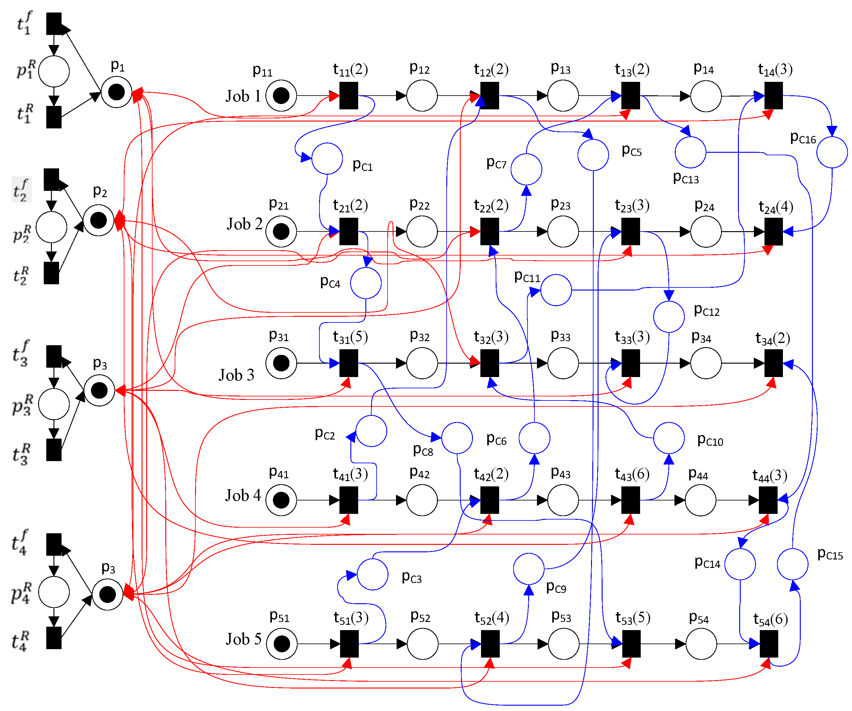
Case study 2: The system has four machines and five components. Each component is subjected to a series of four processes. The data related to this example are depicted in

Table 9. Scheduling data of case study 2.

Part	(Operation, Operation Time, Machine)
1	(1, 2, M1)	(2, 2, M3)	(3, 2, M4)	(4, 3, M2)
2	(1, 2, M1)	(2, 2, M4)	(3, 3, M3)	(4, 4, M2)
3	(1, 5, M1)	(2, 3, M2)	(3, 3, M3)	(4, 2, M4)
4	(1, 3, M3)	(2, 2, M4)	(3, 6, M2)	(4, 3, M4)
5	(1, 3, M2)	(2, 4, M3)	(3, 5, M1)	(4, 6, M4)

and

Table 10. PdM parameters for the machines presented in case study 2.

Parameter	Machine
	1	2	3	4
$t_m^f$ (hr)	Based on sensor system
$t_m^R$ (hr)	2	3	2	3

.

The minimal compilation time is 25 h. Figure 20 depicts Gantt charts for the results obtained using the proposed MILP model. The optimal sequence of start firing transitions is: t₁₁, t₅₁, t₄₁, t₂₁, t₁₂, t₄₂, t₃₁, t₄₃, t₅₂, t₂₂, t₁₃, t₅₃, t₂₃, t₃₂, t₄₄, t₁₄, t₃₃, t₅₄, t₂₄, t₃₄. The controlled TPN model is displayed in Figure 21.

The proposed approach is applicable to problems of large scale. The number of controllers will be augmented in proportion to the increase in shared resources, and the final result of the developed mathematical model might require the use of heuristic methods to minimize computational time. Despite the fact that most FMS scheduling problems are small, the proposed approach is applied to address larger problems. In order to validate the effectiveness of the proposed approach for more complex, dynamic scheduling problems with unreliable flexible manufacturing systems, it is implemented on a larger scale.

Case study 3: The system consists of 10 different types of parts and 6 machines. Each component is subjected to a series of five processes. The data related to this scenario are depicted in

Table 11. Scheduling data of case study 3.

Part	(Operation, Operation Time, Machine)
1	(1, 3, M1)	(2, 5, M2)	(3, 6, M3)	(4, 7, M4)	(5, 8, M5)
2	(1, 8, M3)	(2, 4, M1)	(3, 9, M2)	(4, 6, M6)	(5, 5, M6)
3	(1, 2, M1)	(2, 7, M3)	(3, 5, M1)	(4, 4, M5)	(5, 6, M4)
4	(1, 3, M1)	(2, 2, M2)	(3, 6, M2)	(4, 3, M4)	(5, 2, M5)
5	(1, 5, M6)	(2, 4, M3)	(3, 6, M1)	(4, 7, M2)	(5, 5, M5)
6	(1, 6, M5)	(2, 1, M6)	(3, 8, M6)	(4, 9, M4)	(5, 7, M5)
7	(1, 6, M1)	(2, 5, M2)	(3, 9, M3)	(4, 8, M4)	(5, 7, M6)
8	(1, 5, M5)	(2, 4, M4)	(3, 3, M3)	(4, 4, M2)	(5, 5, M1)
9	(1, 6, M6)	(2, 7, M6)	(3, 7, M4)	(4, 6, M1)	(5, 5, M5)
10	(1, 6, M4)	(2, 5, M3)	(3, 4, M2)	(4, 5, M5)	(5, 6, M6)

and

Table 12. PdM parameters for the machines presented in case study 3.

Parameter	Machine
	1	2	3	4	5	6
$t_m^f$ (hr)	Based on sensor system
$t_m^R$ (hr)	5	3	1	1	2	2

. Figure 22 depicts the optimal schedule for this problem. The minimal cycle time is 64 units of time.

Table 13. Performance of the developed model in all case studies.

Parameter	Case Study
	1	2	3
No. of Parts	3	5	10
No. of Machines	2	4	6
CPU time (second)	2	8	5160

illustrates the size and efficiency of the proposed approach across all of the studies. It demonstrates that the proposed approach includes a greater number of variables and constraints when the problem size is larger. Furthermore, the CPU processing time undergoes a significant increase as the problem size is increased. Thus, the scheduling problem is a complicated and NP-complete problem with a combinatorial structure.

5. Conclusions

This paper presents a method for generating MILP models using timed Petri nets. The method is designed to address the dynamic scheduling problems in UFMSs’ complex industrial conditions. The objective is to construct TPN models using the IoT for the PdM configuration of mechanical equipment in the dynamic scheduling problem of UFMSs to determine the optimal production cycle time. The effectiveness of the proposed approach is demonstrated through several computational instances. The main contributions of the proposed method are as follows:

• It can methodically build MILP instances based on TPN models for UFMSs under complex operational conditions such as concurrency, conflicts, resource sharing, and sequential processes, which can be applied in practical scenarios.
• It provides a hybrid approach that integrates the TPN, the PdM configuration, and the IoT to predict and prevent early mechanical equipment failures in UFMSs, thereby avoiding disruptions to the scheduled operations of other UFMSs.
• The optimal solution for the UFMS scheduling problem obtained from MILP can be converted into a system controller to guarantee the execution of the resulting sequence.

The following is a list of the significant results of the proposed method:

• The computational results are better in terms of the quality of the obtained solutions.
• It enables faster, optimal decision-making in DSP and solves instances for up to 10 parts and 6 machines.
• It is capable of handling all unreliable machines in the UFMSs, and it is perfectly adequate to reach a solution in an acceptable CPU time.

While the current optimization solvers, such as LINGO and high-performance computers, are capable of solving large-scale scheduling problems with significant CPU time, there is a need for approximate approaches such as GA, ACO, PSO, SA, and TS to address these scheduling problems. This will be the focus of future research in this field. Furthermore, our objective is to expand our approach to address optimization issues that involve uncertainty. Stochastic TPNs can be applied to address uncertainty and formulate stochastic optimization problems based on PN models.

References

1. Kaid, H.; Al-Ahmari, A.; Li, Z.; Ameen, W. An Improved Synthesis Method Based on ILPP and Colored Petri Net for Liveness Enforcing Controller of Flexible Manufacturing Systems. IEEE Access 2022, 10, 68570–68581. [Google Scholar] [CrossRef]
2. Chen, Y.; Li, Z.; Al-Ahmari, A. Nonpure Petri net supervisors for optimal deadlock control of flexible manufacturing systems. IEEE Trans. Syst. Man Cybern. Syst. 2012, 43, 252–265. [Google Scholar] [CrossRef]
3. Stecke, K.E. Design, planning, scheduling, and control problems of flexible manufacturing systems. Ann. Oper. Res. 1985, 3, 1–12. [Google Scholar] [CrossRef]
4. Lewis, H.R. Michael R. Garey and David S. Johnson. Computers and intractability. A guide to the theory of NP-completeness. W. H. Freeman and Company, San Francisco1979, x + 338 pp. J. Symb. Log. 1983, 48, 498–500. [Google Scholar] [CrossRef]
5. Modibbo, U.M.; Raghav, Y.S.; Hassan, M.; Mijinyawa, M. A Critical Review on the Applications of Optimization Techniques in the UN Sustainable Development Goals. In Proceedings of the 2021 2nd International Conference on Intelligent Engineering and Management (ICIEM), London, UK, 28–30 April 2021; pp. 572–576. [Google Scholar]
6. Modibbo, U.M.; Ali, I.; Ahmed, A. Multi-objective optimization modelling for analysing sustainable development goals of Nigeria: Agenda 2030. Environ. Dev. Sustain. 2021, 23, 9529–9563. [Google Scholar] [CrossRef]
7. Emrouznejad, A. Big Data Optimization: Recent Developments and Challenges; Springer: Berlin/Heidelberg, Germany, 2016; Volume 18. [Google Scholar]
8. Brouer, B.D.; Karsten, C.V.; Pisinger, D. Big data optimization in maritime logistics. In Big Data Optimization: Recent Developments and Challenges; Springer: Berlin/Heidelberg, Germany, 2016; pp. 319–344. [Google Scholar]
9. Abualigah, L.; Gandomi, A.H.; Elaziz, M.A.; Hamad, H.A.; Omari, M.; Alshinwan, M.; Khasawneh, A.M. Advances in meta-heuristic optimization algorithms in big data text clustering. Electronics 2021, 10, 101. [Google Scholar] [CrossRef]
10. Ibaraki, T. Integer programming formulation of combinatorial optimization problems. Discret. Math. 1976, 16, 39–52. [Google Scholar] [CrossRef]
11. Kantor, I.; Robineau, J.-L.; Bütün, H.; Marechal, F. A mixed-integer linear programming formulation for optimizing multi-scale material and energy integration. Front. Energy Res. 2020, 8, 49. [Google Scholar] [CrossRef]
12. Al-Ahmari, A.; Kaid, H.; Li, Z.; Wu, N.; El-Tamimi, A.-A.; Qiao, Y. A New MINLP Continuous Time Formulation for Scheduling Optimization of Oil Refinery with Unreliable CDUs. Math. Probl. Eng. 2022, 2022, 1298495. [Google Scholar] [CrossRef]
13. Liu, J.; MacCarthy, B.L. A global MILP model for FMS scheduling. Eur. J. Oper. Res. 1997, 100, 441–453. [Google Scholar] [CrossRef]
14. Sankar, S.S.; Ponnanbalam, S.; Rajendran, C. A multiobjective genetic algorithm for scheduling a flexible manufacturing system. Int. J. Adv. Manuf. Technol. 2003, 22, 229–236. [Google Scholar] [CrossRef]
15. T Taghavifard, M.; Heydar, M.; S Mousavi, S. A genetic algorithm for scheduling flexible manufacturing cells. J. Appl. Sci. 2009, 9, 97–104. [Google Scholar] [CrossRef]
16. Candan, G.; Yazgan, H.R. Genetic algorithm parameter optimisation using Taguchi method for a flexible manufacturing system scheduling problem. Int. J. Prod. Res. 2015, 53, 897–915. [Google Scholar] [CrossRef]
17. Sharma, D.; Singh, V.; Sharma, C. GA based scheduling of FMS using roulette wheel selection process. In Proceedings of the International Conference on Soft Computing for Problem Solving (SocProS 2011), Roorkee, India, 20–22 December 2011; Volume 2, pp. 931–940. [Google Scholar]
18. Udhayakumar, P.; Kumanan, S. Some metaheuristic approaches for optimising tardiness of job and tool in a flexible manufacturing system. Int. J. Adv. Oper. Manag. 2012, 4, 219–252. [Google Scholar] [CrossRef]
19. Udhayakumar, P.; Kumanan, S. Sequencing and scheduling of job and tool in a flexible manufacturing system using ant colony optimization algorithm. Int. J. Adv. Manuf. Technol. 2010, 50, 1075–1084. [Google Scholar] [CrossRef]
20. Jerald, J.; Asokan, P.; Prabaharan, G.; Saravanan, R. Scheduling optimisation of flexible manufacturing systems using particle swarm optimisation algorithm. Int. J. Adv. Manuf. Technol. 2005, 25, 964–971. [Google Scholar] [CrossRef]
21. Zhang, C.Y.; Li, P.; Rao, Y.; Guan, Z. A very fast TS/SA algorithm for the job shop scheduling problem. Comput. Oper. Res. 2008, 35, 282–294. [Google Scholar] [CrossRef]
22. Tiwari, M.K.; Kumar, S.; Shankar, R. Solving part-type selection and operation allocation problems in an FMS: An approach using constraints-based fast simulated annealing algorithm. IEEE Trans. Syst. Man Cybern. Part A: Syst. Hum. 2006, 36, 1170–1184. [Google Scholar] [CrossRef]
23. Pitts, R., Jr.; Ventura, J.A. Scheduling flexible manufacturing cells using Tabu Search. Int. J. Prod. Res. 2009, 47, 6907–6928. [Google Scholar] [CrossRef]
24. Sarma, U.; Kant, S.; Rai, R.; Tiwari, M. Modelling the machine loading problem of FMSs and its solution using a tabu-search-based heuristic. Int. J. Comput. Integr. Manuf. 2002, 15, 285–295. [Google Scholar] [CrossRef]
25. Gholami, M.; Zandieh, M. Integrating simulation and genetic algorithm to schedule a dynamic flexible job shop. J. Intell. Manuf. 2009, 20, 481–498. [Google Scholar] [CrossRef]
26. Pergher, I.; Frej, E.A.; Roselli, L.R.P.; de Almeida, A.T. Integrating simulation and FITradeoff method for scheduling rules selection in job-shop production systems. Int. J. Prod. Econ. 2020, 227, 107669. [Google Scholar] [CrossRef]
27. Thenarasu, M.; Rameshkumar, K.; Di Mascolo, M.; Anbuudayasankar, S.P. Multi-criteria scheduling of realistic flexible job shop: A novel approach for integrating simulation modelling and multi-criteria decision making. Int. J. Prod. Res. 2024, 62, 336–358. [Google Scholar] [CrossRef]
28. Bihari, M.; Kane, P. Evaluation and Improvement of Makespan Time of Flexible Job Shop Problem Using Various Dispatching Rules—A Case Study. In Proceedings of the Advances in Mechanical Engineering: Select Proceedings of ICAME 2020, Makassar, Indonesia, 14–15 October 2020; pp. 611–617. [Google Scholar]
29. Balog, M.; Dupláková, D.; Szilágyi, E.; Mindaš, M.; Knapcikova, L. Optimization of time structures in manufacturing management by using scheduling software Lekin. TEM J. 2016, 5, 319. [Google Scholar]
30. Murata, T. Petri nets: Properties, analysis and applications. Proc. IEEE 1989, 77, 541–580. [Google Scholar] [CrossRef]
31. Richard, P. Modelling integer linear programs with Petri nets. RAIRO-Oper. Res. 2000, 34, 305–312. [Google Scholar] [CrossRef]
32. Nakamura, M.; Tengan, T.; Yoshida, T. A Petri net approach to generate integer linear programming problems. IEICE Trans. Fundam. Electron. Commun. Comput. Sci. 2019, 102, 389–398. [Google Scholar] [CrossRef]
33. Tuncel, G.; Bayhan, G.M. Applications of Petri nets in production scheduling: A review. Int. J. Adv. Manuf. Technol. 2007, 34, 762–773. [Google Scholar] [CrossRef]
34. Wu, N.; Chu, F.; Chu, C.; Zhou, M. Petri net modeling and cycle-time analysis of dual-arm cluster tools with wafer revisiting. IEEE Trans. Syst. Man Cybern. Syst. 2012, 43, 196–207. [Google Scholar] [CrossRef]
35. Wu, N.; Zhou, M.; Chu, F.; Chu, C. A Petri-net-based scheduling strategy for dual-arm cluster tools with wafer revisiting. IEEE Trans. Syst. Man Cybern. Syst. 2013, 43, 1182–1194. [Google Scholar] [CrossRef]
36. Qiao, Y.; Wu, N.; Zhou, M. Scheduling of dual-arm cluster tools with wafer revisiting and residency time constraints. IEEE Trans. Ind. Inform. 2013, 10, 286–300. [Google Scholar] [CrossRef]
37. Qiao, Y.; Wu, N.; Zhou, M. A Petri net-based novel scheduling approach and its cycle time analysis for dual-arm cluster tools with wafer revisiting. IEEE Trans. Semicond. Manuf. 2012, 26, 100–110. [Google Scholar] [CrossRef]
38. Zhou, M.; McDermott, K.; Patel, P.A. Petri net synthesis and analysis of a flexible manufacturing system cell. Syst. Man Cybern. IEEE Trans. 1993, 23, 523–531. [Google Scholar] [CrossRef]
39. Zhou, M.; Chiu, H.-S.; Xiong, H.H. Petri net scheduling of FMS using branch and bound method. In Proceedings of the IECON’95—21st Annual Conference on IEEE Industrial Electronics, Orlando, FL, USA, 6–10 November 1995; pp. 211–216. [Google Scholar]
40. Artigues, C.; Roubellat, F. A Petri net model and a general method for on and off-line multi-resource shop floor scheduling with setup times. Int. J. Prod. Econ. 2001, 74, 63–75. [Google Scholar] [CrossRef]
41. Mejía, G.; Odrey, N.G. An approach using Petri nets and improved heuristic search for manufacturing system scheduling. J. Manuf. Syst. 2005, 24, 79–92. [Google Scholar] [CrossRef]
42. Zhang, W.; Freiheit, T.; Yang, H. Dynamic scheduling in flexible assembly system based on timed Petri nets model. Robot. Comput.-Integr. Manuf. 2005, 21, 550–558. [Google Scholar] [CrossRef]
43. Kim, Y.W.; Suzuki, T.; Narikiyo, T. FMS scheduling based on timed Petri Net model and reactive graph search. Appl. Math. Model. 2007, 31, 955–970. [Google Scholar] [CrossRef]
44. Lee, J.; Lee, J.S. Heuristic search for scheduling flexible manufacturing systems using lower bound reachability matrix. Comput. Ind. Eng. 2010, 59, 799–806. [Google Scholar] [CrossRef]
45. Wang, Q.; Wang, Z. Hybrid heuristic search based on Petri net for FMS scheduling. Energy Procedia 2012, 17, 506–512. [Google Scholar] [CrossRef]
46. Kammoun, M.A.; Ezzeddine, W.; Rezg, N.; Achour, Z. FMS scheduling under availability constraint with supervisor based on timed Petri nets. Appl. Sci. 2017, 7, 399. [Google Scholar] [CrossRef]
47. Xu, G.; Chen, Y. Petri-Net-Based Scheduling of Flexible Manufacturing Systems Using an Estimate Function. Symmetry 2022, 14, 1052. [Google Scholar] [CrossRef]
48. Ravidas, S.; Lekidis, A.; Paci, F.; Zannone, N. Access control in Internet-of-Things: A survey. J. Netw. Comput. Appl. 2019, 144, 79–101. [Google Scholar] [CrossRef]
49. Ray, P.P. A survey on Internet of Things architectures. J. King Saud Univ. Comput. Inf. Sci. 2018, 30, 291–319. [Google Scholar]
50. Asghari, P.; Rahmani, A.M.; Javadi, H.H.S. Internet of Things applications: A systematic review. Comput. Netw. 2019, 148, 241–261. [Google Scholar] [CrossRef]
51. Cachada, A.; Barbosa, J.; Leitão, P.; Alves, A.; Alves, L.; Teixeira, J.; Teixeira, C. Using internet of things technologies for an efficient data collection in maintenance 4.0. In Proceedings of the 2019 IEEE International Conference on Industrial Cyber Physical Systems (ICPS), Taipei, Taiwan, 6–9 May 2019; pp. 113–118. [Google Scholar]
52. Niyonambaza, I.; Zennaro, M.; Uwitonze, A. Predictive maintenance (Pdm) structure using internet of things (iot) for mechanical equipment used into hospitals in Rwanda. Future Internet 2020, 12, 224. [Google Scholar] [CrossRef]
53. Kaid, H.; Al-Ahmari, A.; Alqahtani, K.N. Fault Detection, Diagnostics, and Treatment in Automated Manufacturing Systems Using Internet of Things and Colored Petri Nets. Machines 2023, 11, 173. [Google Scholar] [CrossRef]
54. Mobley, R.K. Maintenance Fundamentals; Elsevier: Amsterdam, The Netherlands, 2011. [Google Scholar]
55. Iadanza, E.; Gonnelli, V.; Satta, F.; Gherardelli, M. Evidence-based medical equipment management: A convenient implementation. Med. Biol. Eng. Comput. 2019, 57, 2215–2230. [Google Scholar] [CrossRef]
56. Kaid, H.; Al-Ahmari, A.; Li, Z.; Ameen, W. Deadlock Control and Fault Detection and Treatment in Reconfigurable Manufacturing Systems Using Colored Resource-Oriented Petri Nets Based on Neural Network. IEEE Access 2021, 9, 84932–84947. [Google Scholar] [CrossRef]
57. Agogino, A.; Goebel, K.; Mill Data Set. BEST lab, UC Berkeley. NASA Ames Prognostics Data Repository. NASA Ames: Moffett Field, CA, USA, 2007. Available online: https://ti.arc.nasa.gov/project/prognostic-data-repository (accessed on 1 December 2022).
58. Davidrajuh, R. Modeling Discrete-Event Systems with GPenSIM: An Introduction; Springer: Berlin/Heidelberg, Germany, 2018. [Google Scholar]
Figure 2. An example of a timed Petri net.
Machines 12 00192 g002
Figure 3. An example of an FMS.
Machines 12 00192 g003
Figure 4. A timed PN model of the system shown in Figure 3.
Machines 12 00192 g004
Figure 5. Resources failure detection flowchart.
Machines 12 00192 g005
Figure 6. Estimation resource failure time using IoT.
Machines 12 00192 g006
Figure 7. Estimating resource failure time and recovery net using the IoT for Figure 6.
Machines 12 00192 g007
Figure 8. An example of the completion time of an operation for a job.
Machines 12 00192 g008
Figure 9. Start and end of operations for job i (operations k and l).
Machines 12 00192 g009
Figure 10. Representation of two independent operations for the same job type.
Machines 12 00192 g010
Figure 11. Shared machine in an FMS for jobs i and j.
Machines 12 00192 g011
Figure 12. Representation of maintenance period for machine in an FMS based on IoT.
Machines 12 00192 g012
Figure 13. An illustrative example of an FMS.
Machines 12 00192 g013
Figure 14. A timed PN model of the system shown in Figure 13.
Machines 12 00192 g014
Figure 15. Data collected by sensors to monitor the condition of the tool used in the model depicted in Figure 14.
Machines 12 00192 g015
Figure 16. The optimal schedule for the illustrative example.
Machines 12 00192 g016
Figure 17. The controlled TPN for the model shown in Figure 14.
Machines 12 00192 g017
Figure 18. The optimal schedule for case study 1.
Machines 12 00192 g018
Figure 19. The controlled TPN for the system in case study 1.
Machines 12 00192 g019
Figure 20. The optimal schedule for case study 2.
Machines 12 00192 g020
Figure 21. The controlled TPN for the system in case study 2.
Machines 12 00192 g021
Figure 22. The optimal schedule for case study 3.
Machines 12 00192 g022