
Enhancing Real-Time Kinematic Relative Positioning for Unmanned Aerial Vehicles

1
Research Institute of Science and Technology, Hongik University, Seoul 04055, Republic of Korea
2
PGM Seeker R&D, LIG Nex1, Yongin 16911, Republic of Korea
3
Department of Mechanical Engineering, Hongik University, Seoul 04055, Republic of Korea
4
Department of Mechanical & System Design Engineering, Hongik University, Seoul 04055, Republic of Korea
*
Author to whom correspondence should be addressed.
Machines 2024, 12(3), 202; https://doi.org/10.3390/machines12030202
Submission received: 11 February 2024
/
Revised: 17 March 2024
/
Accepted: 18 March 2024
/
Published: 19 March 2024
(This article belongs to the Special Issue Autonomous Navigation of Mobile Robots and UAV)
Abstract
:Real-time kinematic (RTK) positioning of the global navigation satellite systems (GNSS) is used to provide centimeter-level positioning accuracy. There are several ways to implement RTK but a Kalman filter-based RTK is preferred because of its superior capability to resolve GNSS carrier phase integer ambiguities. However, the positioning performance of the Kalman filter-based RTK is often compromised by various factors when it comes to determining a precise relative position vector between moving unmanned aerial vehicles (UAVs) equipped with low-cost GNSS receivers and antennas, where the locations of both GNSS antennas are not accurately known and change over time. Some of the critical factors that lead to a high rate of incorrect resolutions of carrier phase integer ambiguities are measurement time differences between GNSS receivers, frequent cycle slips with high noise in code and carrier phase measurements, and an improper Kalman filter gain due to a newly risen satellite. In this paper, effective methods to deal with those factors to achieve a seamless Kalman filter-based RTK performance in moving UAVs are presented. Using our extensive 45 flight tests data sets, conducted over a duration of 3 to 12 min, the RTK positioning results showed that the root-mean-square position error (RMSE) decreased by up to 95.13%, with an average of 65.31%, and that the percentage of epochs that passed the ratio test, which is the most common method for validating double differenced carrier phase integer ambiguity resolution, increased by up to 130%, with an average of 23.54%.
1. Introduction
Numerous applications, including construction, surveying, agriculture, and autonomous vehicles, which demand centimeter-level precision, necessitate precise relative positioning. Real-time kinematic (RTK) systems based on the carrier-based differential global navigation satellite system (GNSS) have satisfied these extremely stringent accuracy requirements [1,2,3,4]. An RTK system typically uses double difference (DD) code and carrier phase measurements of the base and rover receivers to achieve centimeter-level relative positioning accuracy [5]. To use carrier phase measurements as precise ranging sources, integer ambiguities in the carrier phase measurements must be resolved and the high level of positioning accuracy is possible only when the integer ambiguities associated with the double difference measurements are correctly resolved. Among various methods for integer ambiguity resolution and validation [6,7], Least-squares Ambiguity Decorrelation Adjustment (LAMBDA) algorithms [8,9,10] with ratio test have gained the most popularity.
While a typical RTK system comprises a static reference receiver and a rover, there are instances where a moving reference station is necessary for RTK applications. Pervan et al., developed a navigation architecture for ship-relative positioning during aircraft carrier landings, utilizing a moving baseline RTK [11,12,13]. Related to that, Khanafseh devised fault detection methods for reference receivers and formulated protection level equations specific to ship-relative positioning [14,15,16]. Kim et al. introduced methods enabling precise operations of ground vehicles and drones solely through moving baseline RTK, extending the benefits of RTK through correction data transmission from ground vehicles [17]. Harish et al. proposed positioning algorithms for single-frequency multi-constellation GNSS systems based on moving baseline RTK [18]. Additionally, Xi et al. applied moving baseline RTK principles to address the health monitoring of bridges, proposing suitable measurement models for the task [19].
Regardless of whether the base station remains stationary [20] or is in motion, both LAMBDA and ratio tests are equally capable of resolving and validating integer ambiguities. Furthermore, while resolving integer ambiguities allows for the computation of the relative position vector between the base station and a rover in a similar manner, it is essential to note that achieving the same level of RTK performance as with a static base station may prove challenging for small unmanned aerial vehicles (UAVs) having low-cost GNSS receivers and antenna. This difficulty arises due to dynamic baseline changes experienced by UAVs, compounded by the large noise levels in code and carrier phase measurements. Also, considerable differences in measurement times between GNSS receivers may exist. Furthermore, frequent satellite inclusion and exclusion may occur during maneuvers, potentially resulting in poor performance of an RTK process. In summary, compared to the relatively straightforward scenario involving a stationary base station, achieving RTK performance between moving UAVs with a dynamic baseline poses greater challenges. Addressing these challenges comprehensively is crucial for ensuring seamless RTK performance and should consider the below problems that have been rarely discussed in the literature, as far as the author is aware.
- GNSS Measurements Time Synchronization between UAVs;
- Cycle slip detection strategy for a UAV;
- Adopting Dual Kalman filter (KF) structure to cope with ratio test failures owing to relatively inaccurate estimates of newly added states.
First, if there is a relatively large difference in measurement time when processing measurements from low-cost receivers on UAVs, the difference should be adjusted as if they were measured simultaneously. The ranging measurement offsets resulting from this time difference are not a problem when the location of the base station is precisely known [21]. However, for a moving-baseline RTK, it is crucial to correct the measurement time difference to obtain an accurate relative position vector.
Secondly, a KF-based RTK algorithm outperforms the single-epoch least-squares method [22,23] in terms of resolving integer ambiguities by LAMBDA due to its more precise integer ambiguity estimates and corresponding covariance matrix. The KF-based RTK measurement model assumes the consistency of integer ambiguities between two consecutive epochs. Therefore, a reliable cycle slip detection method is necessary to handle these changes in carrier phase measurements. Although some GNSS receivers generate a loss of lock indicator (LLI) to report cycle slip measurements, LLI may contain incorrect information [24]. Therefore, it is not recommended to rely solely on LLI for cycle slip detection, and a robust cycle slip detection strategy for single and dual-frequency measurements is required. Moreover, for UAVs in motion, the noise level of the cycle slip test metrics can be significantly higher than that for static ground receivers. As a result, this study developed cycle slip detection thresholds for UAVs based on the test statistics of flight test data to avoid unnecessary and frequent exclusion of carrier phase measurements.
Thirdly, an additional problem with implementing a KF-based RTK is that the ratio tests of the estimated integer ambiguities from LAMBDA often fail when new GNSS measurements are included with an initial estimate of the state values and their covariance. As a result, it can take several tens of epochs for the resolved integer ambiguities with the newly incorporated satellites to pass the ratio test threshold. Therefore, in this paper, we briefly explained why the ratio test can fail in the presence of newly added KF states and introduced a dual KF structure to solve this problem.
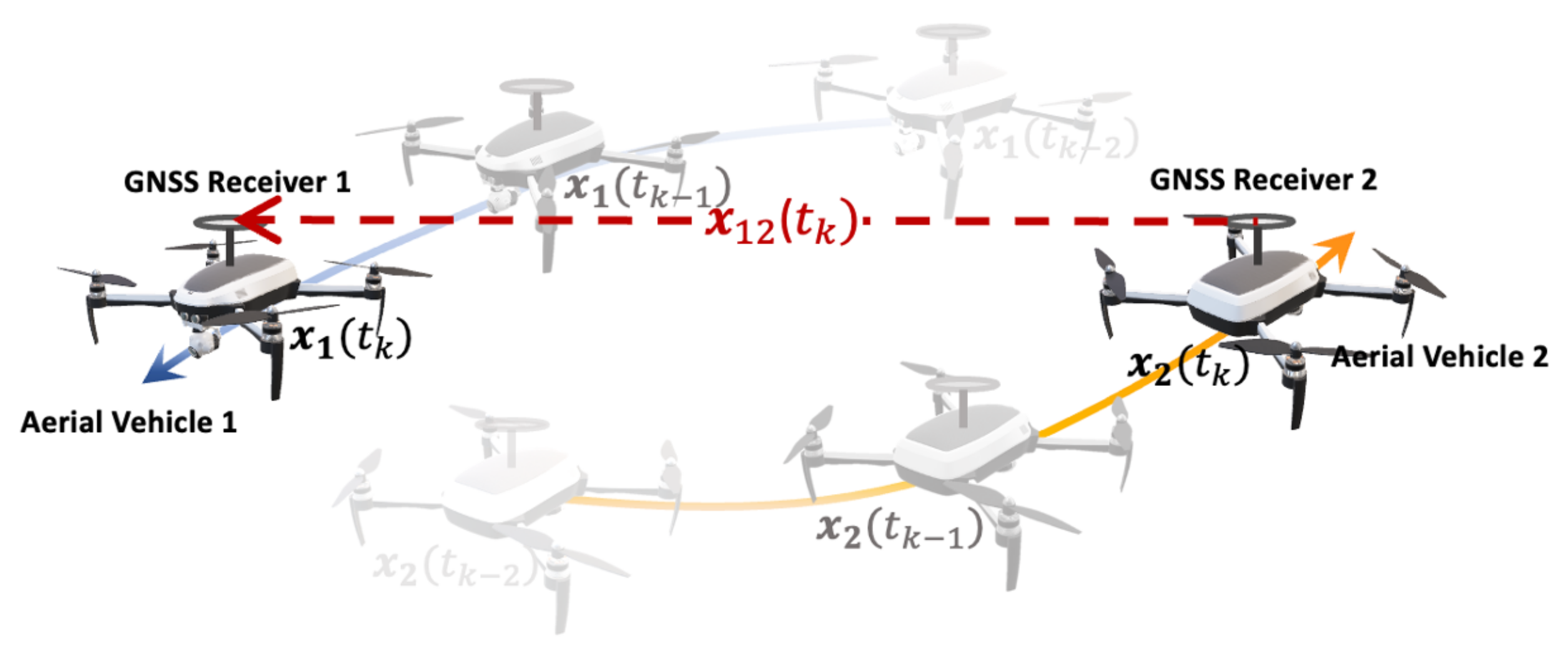
The limited exploration of the aforementioned three problems in previous studies is attributed to the understanding that no single algorithm can address them all. Instead, they are best solved by distinct logical approaches within the RTK process. The primary contribution of this work lies in identifying the key factors impeding the attainment of centimeter-level RTK position solutions when dealing with two UAVs flying in close proximity. Additionally, it proposes a comprehensive RTK process aimed at addressing these challenges, incorporating measurement time synchronizations, cycle slip detection methods tailored for small UAVs, and dual KF structures. These proposed methods were validated through extensive flight test data. Note that the overall methods proposed in this study primarily focused on a short baseline RTK method for situations where two UAVs equipped with GNSS receivers and antennas are moving, as shown in Figure 1.
This paper is structured as follows: Section 2 outlines the GNSS measurement model and the time synchronization process between measurements from two different GNSS receivers. Section 3 describes techniques for detecting single- and dual-frequency GNSS carrier phase cycle slips for a UAV. In Section 4, the implementation of a dual KF structure is discussed with its rationales, in order to derive an accurate and robust navigation solution when the number of GNSS measurements varies and to cope with ratio test failures. Section 5 evaluates the performance improvements of the proposed methods using the flight test data collected from UAVs, followed by conclusions in Section 6.
2. Gnss Measurements Pre-Processing and Time Synchronization
The GNSS measurements pre-processing procedure, as shown in Figure 2, involves cycle slip detection and measurement time synchronization between the two GNSS receivers. To ensure accurate time synchronization of the GNSS measurements, only measurements with a carrier-to-noise ratio (C/N0) of more than 35 dBHz and that passed the cycle slip tests were used in the RTK process.
The GNSS observables of satellite k at f frequency for receiver i can be formulated as follows
where and are carrier phase , code and Doppler frequency measurements of a GNSS signal, respectively. Here, is a geometric range between the receiver i and a satellite k. and refer to ionospheric and tropospheric delays. and are the receiver and satellite clock biases, respectively. and are signal wavelength and integer ambiguity of carrier phase measurements. Each measurement noise and errors are denoted as , , and .
As we are dealing with a short baseline RTK problem where the distance between two receivers is less than several kilometers, a single difference of GNSS measurements between receiver i and receiver j for satellite k is as follows:
Common satellite clock biases and ionospheric and tropospheric delays are eliminated using a single difference between receivers. Then, the receiver clock biases are removed by double-differencing between satellite k and pivot satellite l as follows
where stands for a user-to-satellite line-of-sight unit vector and is a relative position vector between receiver i and receiver j. Under the short baseline assumption, has been considered virtually the same as .
In contrast to the ideal case where both GNSS measurements are received simultaneously at the exact same time, subtle measurement time differences between two distinct GNSS receivers may exist in practical scenarios as shown in Figure 3. Having additional unmodeled biases in the GNSS measurements may lead to a false resolution of LAMBDA if not corrected. Therefore, the time differences between the measurements should be adjusted.
The following equations show how the carrier and code measurements at time from receiver j are synchronized to receiver i at time using Doppler frequency measurements.
The times and are computed by subtracting each receiver clock bias from the GNSS measurement observation time. In cases where Doppler frequency measurements are unavailable, the time-differenced value of the cycle-slip-free carrier phase measurements can be used as an alternative.
3. Cycle Slip Detection Strategy for a UAV
Cycle slips can be detected by differencing GNSS measurements gathered from two closely located receivers to form DD measurements, eliminating many common measurement errors [25,26,27,28,29]. However, in this paper, a cycle slip detection capability has been integrated into a single GNSS receiver to simplify implementation and ensure robust independent operation. A common method for cycle slip detection in a single GNSS receiver uses a combination of single- or dual-frequency codes and carrier phase measurements [30,31].
Although there are many cycle slip detection methods in the literature, carrier phase measurement characteristics should be considered to obtain proper cycle slip detection performance for a relatively low-cost GNSS receiver on small rotary-wing vehicles. In this work, we developed cycle slip detection strategies based on the test statistics of the following three cycle slip detection methods obtained through flight test data.
- Time-Differenced Dual-Frequency carrier phase Combination (TDDFC);
- Doppler-Aided Cycle Slip Detection (DACSD);
- Time-Differenced Single-Frequency carrier phase Measurements (TDSFM);
GNSS data from GPS, Galileo (GAL), and Beidou (BDS), corresponding to the frequencies and wavelengths listed in Table 1 were collected and used.
3.1. Time-Differenced Dual-Frequency Carrier Phase Combination (TDDFC)
First, TDDFC values are calculated as follows [31]:
where the multipath-induced range errors in each measurement are denoted as . is a differencing operator between successive epochs. Assuming that ionospheric delay can be ignored owing to ionospheric inactivity, Equation (7) can be expressed as follows if the integer ambiguities are the same in consecutive epochs.
Figure 4 shows the TDDFC values from the flight data within the threshold value at which no cycle slips occur. The threshold for is formulated from our flight test data at a false alarm level of using a third-order polynomial equation.
Although the TDDFC thresholds are sufficiently low to detect small cycle slips, there are some particular dual-frequency cycle slip combinations that result in low values of TDDFC such that no cycle slips can be observed. Some examples of these particular combinations and the corresponding TDDFC values are listed in Table 2.
As an example, Figure 5 shows the missed detection probabilities of the TDDFC detector for 39 and 30 cycle slips in and bands, respectively. As shown in Figure 5, all of the TDDFC values of GAL and BDS were smaller than the threshold, indicating that certain cycle slip combinations would be difficult to detect in practice using TDDFC alone. To address these challenges, the DACSD was used in parallel with the TDDFC.
3.2. Doppler-Aided Cycle Slip Detection (DACSD)
DACSD uses time-differenced single-frequency carrier phase and Doppler measurements as the test metric, calculated as follows:
where is the time duration between and .
Figure 6 shows the DACSD values without cycle slips and the derived threshold values.
Due to the large noise level of Doppler measurements from UAVs, the threshold was set to have a false alarm rate of . Here, the thresholds of DACSD were found to be four to six cycles, depending on the elevation angle. Therefore, cycle slip combinations listed in Table 2 can be reliably detected, except for the (1,1) cycle combination. Other monitoring approaches could be used for the (1,1) cycle slip case, including range residual tests, which require further investigation.
3.3. Time-Differenced Single-Frequency Carrier Phase Measurements (TDSFM)
In general, the DACSD can be also used for single-frequency measurements. However, because of its large thresholds, DACSD is recommended for use in conjunction with another test metric. In this study, the use of time-differenced single-frequency carrier phase measurements (TDSFM) [32] was proposed for cycle slip detection of single-frequency-only measurements. To derive the TDSFM metric, the time rate of the carrier phase is modeled as follows:
where dot is a differentiation operator, and are the velocities of the UAV and satellite k, respectively.
To calculate TDSFM, the velocity of the UAV and its clock drifts are computed using dual-frequency measurements that have already passed the TDDFC and DACSD thresholds. Then, can be assumed to be zero, and Equation (10) can be reformulated as follows:
where is an estimated satellite velocity from the broadcast ephemeris data. Using m sets of carrier phase rates that have passed the TDDFC and DACSD tests, and can be determined from the following linear equation:
where
With estimated , denoted as , TDSFM values, , for nth single frequency-only measurements are computed as follows:
collected from flight tests are shown in Figure 7. There was no apparent trend in the TDSFM with respect to the satellite elevation angles, which seemed to be caused by the small number of single-frequency measurement samples. Based on the test statistics, the threshold for is set as a constant of 0.1160 m/s to allow a false alarm rate of . The TDDFC, DACSD, and TDSFM thresholds are summarized in Table 3.
4. Proposed Dual Kalman Filter Structure for RTK and Its Rationales
This section begins with a brief introduction to a conventional KF-based RTK approach with its outcomes. Subsequently, the dual KF structure proposed in this paper and the rationale behind it are investigated.
4.1. Conventional Kalman Filter Based RTK Approach
In Section 3, the preprocessing of GNSS measurements is discussed, such as GNSS measurement selection with the satellite elevation angle and C/N0 of the measurements, the detection of cycle slips, and the time synchronization of GNSS measurements. This section deals with the procedures that remain after the GNSS measurement time synchronization block in Figure 8.
The state vector for a KF-based RTK denoted as includes relative position vector, relative velocity vector, and single differenced integer ambiguities.
Here, , are relative position and velocity vector and () are single differenced integer ambiguities between receiver i and receiver j when m GNSS carrier phase measurements are available. With a discrete state transition matrix from the ()th epoch to the kth epoch, denoted as , the predicted state vector, and its covariance matrix are computed from the previously updated state vector and its covariance matrix.
where
Here, and are predicted state vector and its covariance matrix at the kth epoch, and and are updated state vector and its covariance matrix at the ()th epoch. A constant-velocity model is used for the state transition matrix and is the time duration between the ()th epoch and the kth epoch. refers to the system noise matrix over the time .
When new measurements arrive, KF gain, , which determines weights to the new measurements are calculated as follows
where
Here, is a linearized measurement model that incorporates the matrix in Equation (5), and is a covariance matrix for measurement noise. The initial parameters of the KF were set based on established benchmarks from previous work, particularly referencing [21]. These parameters were subsequently updated through heuristic comparison with results obtained from our experimental data. The matrix converts single differenced integer ambiguities into double differenced integer ambiguities of carrier phase measurements, where is a diagonal matrix composed of wavelengths of the respective carrier phase measurements. Given that each satellite constellation, such as GPS, GAL, and BDS, has its own pivot satellite, the matrix with all of these constellations is formulated as follows:
For example, if the integer ambiguity state of a pivot satellite in the GPS is located at the first element of the single differenced integer vector, is defined as below.
Finally, the KF updates the state and corresponding covariance matrix based on the KF gain with received measurements . To avoid numerical instability of the KF process, the Joseph form of the covariance update equation in [33] is used.
From Equation (21), the estimated states and covariance matrix are re-transformed to derive a float solution of double differenced integer ambiguities.
where
In this equation, the covariance matrix associated with the float solution, , is denoted separately as , while represents the covariance matrix for the updated relative position and velocity vector. Then, the LAMBDA algorithm [10] is applied to compute the so-called fixed integer solutions, , from the float solution and its covariance matrix. This fixed integer solution undergoes a validation process via a well-known ratio test. Employing the widely adopted criteria, if the ratio value exceeds the threshold of three, the final fixed relative position, , and velocity vector, , are calculated as follows:
when the ratio test was not passed, which means the ratio value did not exceed the threshold of 3, the float solution, , was used instead of the fixed solution, .
4.2. Dual Kalman Filter Structure
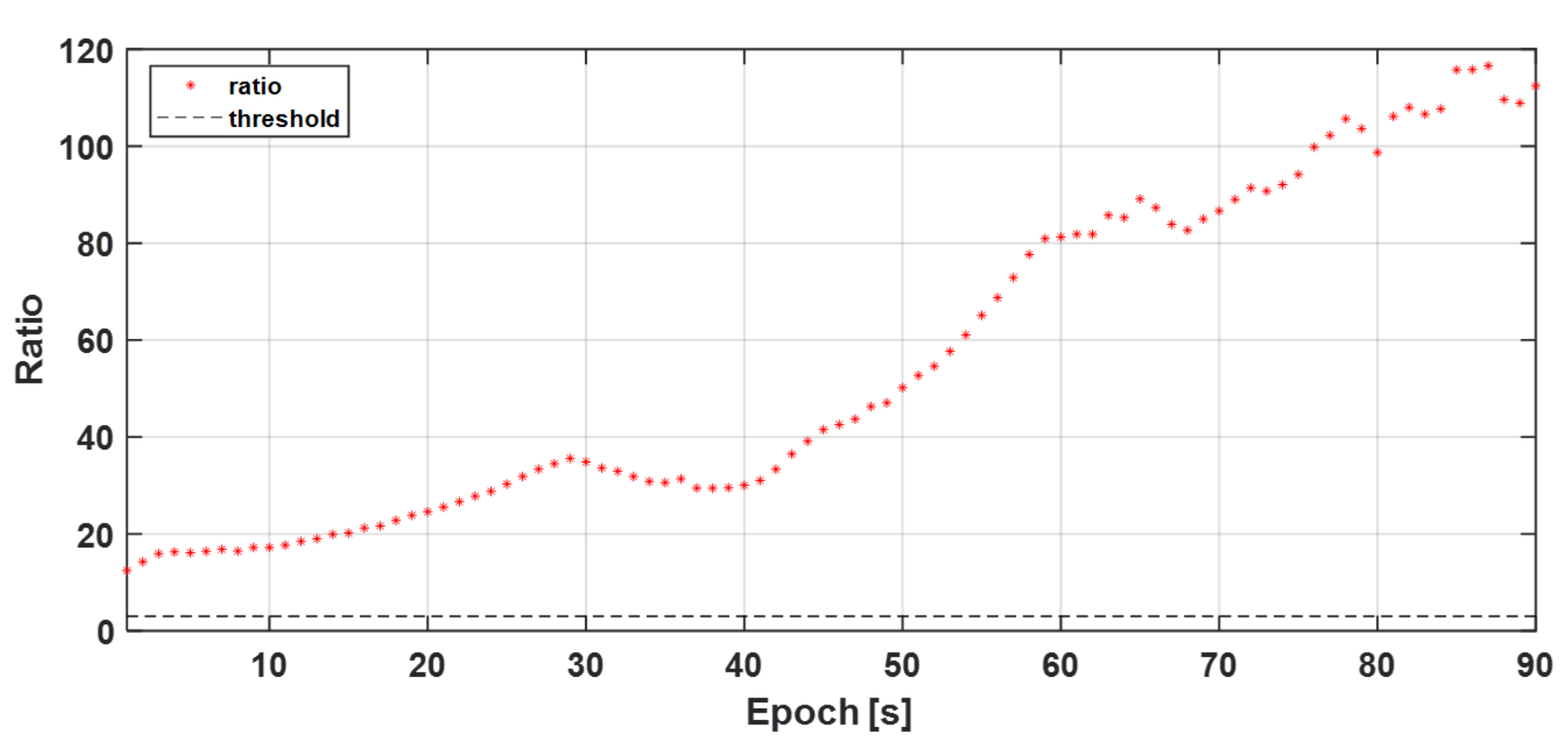
Once the float integer solutions converge in the KF, the integer solutions tend to continuously pass a ratio test with an escalating ratio value, as shown in Figure 9, except in some cases.
One such case is the addition of satellites to the KF, which often causes a ratio test to fail. This subsection discusses the causes of the ratio test failure owing to the newly added satellite and the remedies used in this paper by a dual KF structure.
4.2.1. Analysis of the Effect of a Newly Risen Satellite on the KF and Integer Ambiguity Resolution in LAMBDA
During KF-based RTK operations, satellites may rise or fall. When the satellite falls, the corresponding integer ambiguity state is removed in KF, which usually does not cause a problem if several satellites still remain in view. However, a problematic case occurs when the KF includes additional integer ambiguity (AIA) states to incorporate a newly risen satellite or reintroduce satellites previously excluded due to cycle slips. In this case, a so-called ratio test value, r in Equation (24), could drastically drop below three.
where and are the best and second-best integer vector solutions resulting from LAMBDA.
The reason for the low r is that the AIA states are introduced with a roughly predicted initial value with a large covariance whereas the current integer ambiguity (CIA) states that have been estimated in KF have accurate means with a very small state covariance. The large covariance gap, typically more than several thousand times, between the AIA and CIA states results in a KF gain, K, that places small weights on KF innovations associated with the AIA states. However, the KF gain associated with the CIA states was only slightly affected by the additional satellites. In particular, this characteristic of K prevents the AIA states from being effectively updated by KF innovations, and the updated AIA state float solution would have a similar bias to the roughly estimated initial AIA value. This bias subsequently induces an integer bias in vectors of the best and second-best solutions in LAMBDA.
This KF gain characteristic is best observed by numerical inspections rather than algebraic derivations. A typical KF gain characteristic before and after the inclusion of the AIA state is shown in Figure 10. As shown in Figure 10, the KF gain magnitudes have similar values in two consecutive epochs. The index of the AIA state is 42, and its KF gain magnitude is more than 10 times smaller than most of the gain magnitudes of the other integer states. The integer states with indices 4–6 also have very small gain magnitudes, but these are not of concern as they are already very small before the AIA state is included.
Here, it is interesting to note that the resolved integers for the CIA are usually correct even when r is less than three, and the resolved integer is incorrect for the AIA, whose characteristics are used to develop the proposed dual KF structure. To see these characteristics more clearly, let us first consider the following cost function used in LAMBDA:
where
In the above equations, is a transformation matrix that decorrelates the original integer ambiguity of . denotes a unit lower triangular matrix and is a diagonal matrix with conditional variances of . The LAMBDA search process sequentially determines integer candidates from those with the smallest to those with the largest conditional variances, i.e., a move-down step from to . Once a complete first set of integer vector solution with a tentative minimum cost function has been obtained, the second solution is set identically to the first solution except that the vector element with the largest conditional covariance is added by . The search for the second solution is performed by adding integers in a search space from to , a move-up step. If a lower cost function is found during the move-up steps, the search direction then changes to the move-down steps. The search process is terminated when no further integer candidates are found in the search space.
Now, when an AIA state is introduced into the KF, there are states, and is assigned to the newly added state. Then, the cost function becomes:
Here, because of the large covariance of the AIA state, is much larger than through . Assuming that and in Equations (25) and (28) are very close, then the minimized cost functions in Equations (25) and (28) would also be very close because is negligible in Equation (28). The almost same values of Equations (25) and (28) indicate that the fixed integers of through are essentially identical. Again, would be incorrect and differed by 1 in the best and the second-best integer solution vectors while through are the same in both solutions.
4.2.2. Dual KF Structure Development Strategy
From the above analysis, we can deduce that the approximately predicted initial value and the large covariance of an AIA state must be refined to correctly resolve integer ambiguities with . Thus, it might be beneficial to remove the problematic integer state and wait for it to be refined before passing it to LAMBDA. A convenient and practical approach is to therefore implement a dual KF structure. The dual KF structure consists of a primary main-KF and temp-KF. The main-KF was primarily used for determining position solutions with resolved integer ambiguities. The temp-KF was operated only when the ratio test failed and at least one AIA existed.
The dual KF structure-based RTK procedure is illustrated in Figure 11. The proposed KF procedure starts with a main-KF. In a typical RTK implementation, the main-KF passes the ratio test after some initialization time and results in centimeter-level positioning accuracy. In the course of RTK operation, new satellites can appear and be included in the main-KF. As discussed previously, the ratio test may fail with a high probability if an AIA has been introduced to the main-KF. If the main-KF fails the ratio test, the AIA is excluded and re-updated without the AIA state by temp-KF. Now, a temp-KF without AIA is implemented and used for position solutions instead of the main-KF until the main-KF LAMBDA solution with AIA passes a ratio test owing to the convergent state covariance.
Figure 12 compares the ratios of the main-KF and the temp-KF. In the figure, the ratio of the main-KF alone drops below three when new satellites are included in the KF filter. However, the ratio of the temp-KF is above three.
5. Results
5.1. Experimental Set-Up and Methods
A total of 45 flight test data samples were used to validate the proposed RTK technique with up to four UAVs. Figure 13 shows an example flight path of the four UAVs and one of our UAV testbed used for the flight test. Each UAV followed pre-programmed flight trajectories using a Pixhawk flight controller and a standalone GNSS receiver (3DR, Chula Vista, CA, USA) for about 10 min in a test. The speed of the UAVs was between 1.0 and 3.5 m/s at an altitude of 10 m. During the flight tests, separate Ublox ZED-F9P GNSS receivers (Ublox AG, Thalwil, Switzerland) and Trimble AV17 GNSS antennas (Trimble, Sunnyvale, CA, USA) were mounted on the UAVs to capture dual-frequency code and carrier phase measurements of GPS, GAL, and BDS constellations at a 1 Hz rate. The dual-frequency raw measurements were stored on a memory card within a Raspberry Pi 4 mini computer (Raspberry Pi LTD, Cambridge, England) and subsequently processed to generate RTK position solutions in a post-processing mode using Matlab software version R2022a. To validate the proposed algorithms, the true relative position vectors between the UAVs were determined by subtracting RTK solutions between each UAV and a nearby continuously operating static reference station in Suwon, South Korea, using open-source RTKLIB software version 2.4.3 b34 and TRIMBLE TBC software version 1 [34,35].
5.2. Performance Improvement through Synchronization of Measurement Times
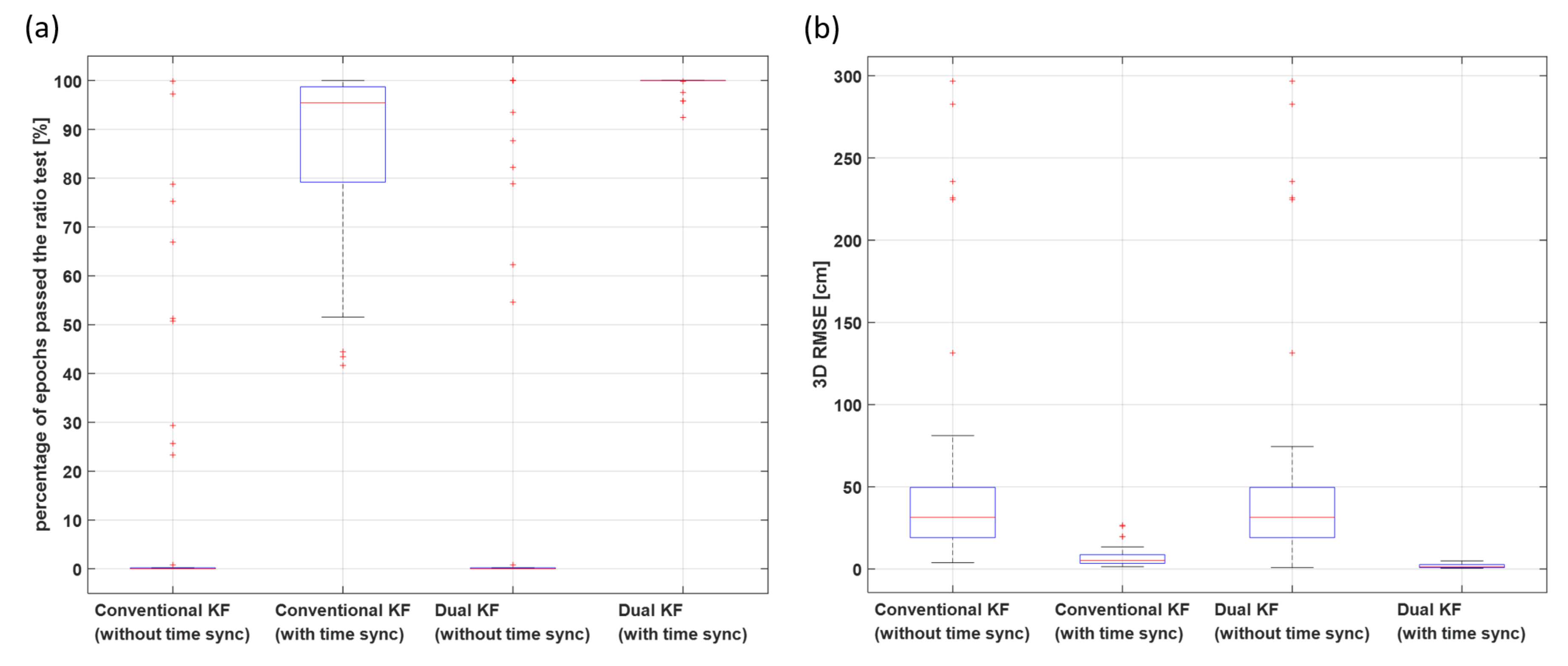
Figure 14 shows the ratios of the test pass rates and the 3D Root Mean Square Errors (RMSE) of the relative positions between the UAVs. The flight test data was used to compare the results of using conventional and dual KFs with and without GNSS measurement time synchronization. The results reveal that neither conventional nor dual KFs without time synchronization can achieve centimeter-level positioning performance. With measurement time synchronization, both KFs had ambiguity fix rates above 40% on all datasets, while without the time synchronization process, both KFs had fix rates of 0% on 34 out of 45 datasets. The average ratio-test pass rate increased from 13.31% to 85.93% for the conventional KF and from 19.11% to 99.59% for the dual KF, representing an overall performance improvement of 545% and 421%, respectively. Also, the average 3D RMSE decreased from 57.96 cm to 7.14 cm for the conventional KF and from 57 cm to 1.93 cm for the dual KF, showing a 3D RMSE reduction of 87.7% and 96.6%, respectively. The difference in RTK performance with and without the time synchronization process is significant, except for a few limited cases where the time difference between the received measurements is sufficiently small to be negligible.
5.3. Performance Improvement via Proposed Cycle Slip Detection Strategy for a UAV
Compared to the GNSS measurements received from a stationary GNSS receiver, we found that the code and carrier phase measurements of a UAV contain a relatively large level of noise. Figure 15a compares experimental distributions of the TDDFC metrics from the static GNSS receivers and the flight test data. Therefore, using the well-known carrier phase measurement noise model derived from static ground receivers in [36] may lead to a significant number of false alarms in detecting cycle slips. The effect of tight thresholds not only reduces the average number of carrier phase measurements, but frequent exclusions and re-introduction of satellites into the KF lead to poor convergence performance overall.
Figure 15b shows the minimum, maximum, and average number of carrier phase measurements remaining after the proposed cycle slip detectors with threshold in [36] and from Table 3, respectively. It can be clearly seen that with the TDDFC threshold in [36], a large amount of GNSS data from moving UAVs would be declared as a cycle-slipped carrier phase and excluded accordingly.
5.4. Performance Improvement via Dual Kalman Filter Structure
Table 4 shows the pass rates of the ratio tests and the 3D RMSE of the relative positions between the UAVs with conventional and dual KFs. In this test, measurement time synchronization and the proposed cycle slip detection approach were implemented in both KFs. Overall, the dual KF performed better than the conventional KF in both aspects. Compared to the conventional KF, average improvements in the ambiguity fix ratio and 3D RMSE of position errors are 23.54 and 65.31 percent, respectively. A total of 43 out of 45 tests showed an improved performance in terms of 3D RMSE reduction along with ratio test pass rate. The remaining two cases had 100 % ratio test pass rates with the conventional KF; thus, there were no advantages to using the dual KF. Although an increase in the ratio test pass rate seemed to result in a reduction in 3D RMSE, the dataset that showed the largest improvement in fix rate differed from the dataset with the largest RMSE reduction. This is because the reduction in 3D RMSE was highly dependent on the overall accuracy of the conventional KF’s float solution, in addition to the ratio test pass rate. The conventional KF produced inaccurate float solutions when it frequently failed the ratio test in the early stages of the KF. Therefore, improving the ratio test pass rate in the early stages of the KF contributed to result in a greater reduction in 3D RMSE for the dual KF structure. With the proposed dual KF structure, all 45 datasets had 3D position RMSE less than 10 cm. Nonetheless, some datasets did not achieve a 100% pass rate on the ratio test, and some fixed solutions had instantaneous 3D position errors over 10 cm. The results suggest that if the ratio test failures were due to problems other than the inclusion of new satellites into the KF, the proposed dual KF structure is subject to the same problems. To address these concerns, implementing partial ambiguity resolution or residual tests needs to be explored in conjunction with the dual KF structure, which will be a topic for our future research.
6. Conclusions
This paper presents effective techniques that improve the RTK performance of moving UAVs. These include measurement time synchronizations and cycle slip detectors for low-cost GNSS receivers on flying vehicles. In addition, the causes of ratio test failure in a typical KF filter-based RTK owing to newly included satellites are discussed, and dual KF structures that overcome these drawbacks are presented. The effectiveness of the proposed algorithms was confirmed using data from 45 UAV flight tests. Without synchronized measurement times, both the conventional and dual Kalman filters exhibited notably low average ratio test pass rates, about 16.21 percent. However, implementing the proposed synchronization method for measurement times, the average ratio test pass rates for the conventional and dual Kalman filters improved significantly by 545 and 421 percent, respectively. Also, the appropriate cycle slip detection metrics and thresholds were introduced, tailored to the measurement characteristics of small UAVs. Through the implementation of these proposed cycle slip detection thresholds, our flight test data showed the prevention of false exclusions of two to six satellites. By employing the suggested measurement time synchronization and cycle slip detection techniques, the dual Kalman filter demonstrated significant enhancements in both the ambiguity fix ratio and 3D RMSE of position errors. Specifically, compared to the conventional KF, the dual KF showed average improvements of 23.54 percent and 65.31 percent, respectively, in these metrics. Overall, the proposed algorithms can be used to improve the RTK solutions of dynamic platforms with low-cost GNSS receivers.
Author Contributions
Conceptualization, E.K. and Y.S. Experiments, C.L., Y.S., Software, C.L., Y.S. All authors have read and agreed to the published version of the manuscript.
Funding
This research was supported by the Unmanned Vehicles Core Technology Research and Development Program through the National Research Foundation of Korea (NRF) and the Unmanned Vehicle Advanced Research Center (UVARC) funded by the Ministry of Science and ICT, Republic of Korea (No. 2020M3C1C1A01086407). This work was also supported by Future Space Navigation & Satellite Research Center through the National Research Foundation funded by the Ministry of Science and ICT, Republic of Korea (2022M1A3C2074404).
Data Availability Statement
Data used for the paper are currently unavailable.
Conflicts of Interest
The authors declare no conflicts of interest.
References
- Sun, H.; Slaughter, D.C.; Ruiz, M.P.; Gliever, C.; Upadhyaya, S.K.; Smith, R.F. RTK GPS mapping of transplanted row crops. Comput. Electron. Agric. 2010, 71, 32–37. [Google Scholar] [CrossRef]
- Varbla, S.; Puust, R.; Ellmann, A. Accuracy assessment of RTK-GNSS equipped UAV conducted as-built surveys for construction site modelling. Surv. Rev. 2020, 53, 477–492. [Google Scholar] [CrossRef]
- Tamura, Y.; Matsui, M.; Pagnini, L.; Ishibashi, R.; Yoshida, A. Measurement of wind-induced response of buildings using RTK-GPS. J. Wind Eng. Ind. Aerodyn. 2002, 90, 1783–1793. [Google Scholar] [CrossRef]
- Meguro, J.; Hashizume, T.; Takiguchi, J.; Kurosaki, R. Development of an autonomous mobile surveillance system using a network-based RTK-GPS. In Proceedings of the 2005 IEEE International Conference on Robotics and Automation, Barcelona, Spain, 18–22 April 2005; pp. 3096–3101. [Google Scholar] [CrossRef]
- Zhao, S.; Cui, X.; Guan, F.; Lu, M. A Kalman Filter-Based Short Baseline RTK Algorithm for Single-Frequency Combination of GPS and BDS. Sensors 2014, 14, 15415–15433. [Google Scholar] [CrossRef] [PubMed]
- Verhagen, S. Integer ambiguity validation: An open problem? GPS Solut. 2004, 8, 36–43. [Google Scholar] [CrossRef]
- Li, T.; Wang, J. Some remarks on GNSS integer ambiguity validation methods. Surv. Rev. 2012, 44, 230–238. [Google Scholar] [CrossRef]
- Jonge, P.D.; Tiberius, C. Integer ambiguity estimation with the lambda method. In GPS Trends in Precise Terrestrial, Airborne, and Spaceborne Applications; Springer: Berlin/Heidelberg, Germany, 1996; pp. 280–284. [Google Scholar] [CrossRef]
- Jonge, P.D.; Tiberius, C. The LAMBDA method for integer ambiguity estimation: Implementation aspects. Publ. Delft Comput. Cent. LGR Ser. 1996, 12, 1–47. [Google Scholar]
- Verhagen, S.; Li, B.; Geodesy, M. LAMBDA Software Package: Matlab Implementation, Version 3.0; Delft University of Technology and Curtin University: Perth, Australia, 2012. [Google Scholar]
- Pervan, B.; Chan, F.C.; Gebre-Egziabher, D.; Pullen, S.A.M.; Enge, P.E.R.; Colby, G. Performance Analysis of Carrier-Phase DGPS Navigation for Shipboard Landing of Aircraft. Navigation 2003, 50, 181–191. [Google Scholar] [CrossRef]
- Pervan, B.; Chan, F.C. System concepts for cycle ambiguity resolution and verification for aircraft carrier landings. In Proceedings of the 14th International Technical Meeting of the Satellite Division of The Institute of Navigation (ION GPS 2001), Salt Lake City, UT, USA, 11–14 September 2001; pp. 1228–1237. [Google Scholar]
- Heo, M.B.; Pervan, B. Carrier phase navigation architecture for shipboard relative GPS. IEEE Trans. Aerosp. Electron. Syst. 2006, 42, 670–679. [Google Scholar]
- Khanafseh, S.; Pervan, B. New approach for calculating position domain integrity risk for cycle resolution in carrier phase navigation systems. IEEE Trans. Aerosp. Electron. Syst. 2010, 46, 296–307. [Google Scholar] [CrossRef]
- Khanafseh, S.; Langel, S.; Pervan, B. H1-integrity of carrier phase navigation algorithms using multiple reference receivers. In Proceedings of the 2009 International Technical Meeting of The Institute of Navigation, Anaheim, CA, USA, 26–28 January 2009; pp. 236–247. [Google Scholar]
- Rife, J.; Khanafseh, S.; Pullen, S.; de Lorenzo, D.; Kim, U.-S.; Koenig, M.; Chiou, T.-Y.; Kempny, B.; Pervan, B. Navigation, interference suppression, and fault monitoring in the sea-based joint precision approach and landing system. Proc. IEEE 2008, 96, 1958–1975. [Google Scholar] [CrossRef]
- Kim, G.; Park, W.; Park, B. Moving Baseline RTK-based Ground Vehicle-Drone Combination System. In Proceedings of the 2024 International Technical Meeting of the Institute of Navigation, Long Beach, CA, USA, 22–25 January 2024; pp. 630–636. [Google Scholar]
- Sridhara, H.S.; Kubo, N.; Kikuchi, R. Single-Frequency Multi-GNSS RTK Positioning for Moving Platform. In Proceedings of the 2015 International Technical Meeting of the Institute of Navigation, Dana Point, CA, USA, 26–28 January 2015; pp. 504–511. [Google Scholar]
- Xi, R.; Jiang, W.; Xuan, W.; Xu, D.; Yang, J.; He, L.; Ma, J. Performance Assessment of Structural Monitoring of a Dedicated High-Speed Railway Bridge Using a Moving-Base RTK-GNSS Method. Remote Sens. 2023, 15, 3132. [Google Scholar] [CrossRef]
- Herrera, A.M.; Suhandri, H.F.; Realini, E.; Reguzzoni, M.; De Lacy, M.C. goGPS: Open-source MATLAB software. GPS Solut. 2016, 20, 595–603. [Google Scholar] [CrossRef]
- Takasu, T.; Yasuda, A. Development of the low-cost RTK-GPS receiver with an open source program package RTKLIB. In Proceedings of the International Symposium on GPS/GNSS, International Convention Center, Jeju, Republic of Korea, 4–6 November 2009; pp. 1–6. [Google Scholar]
- Baroni, L.; Kuga, H.K. Analysis of navigational algorithms for a real time differential GPS system. In Proceedings of the 18th International Congress of Mechanical Engineering, Ouro Preto, Brazil, 6–11 November 2005. [Google Scholar]
- Yujin, S.; Euiho, K. GNSS-based Short Baseline Relative Positioning of Moving Vehicles and Evaluation on its Positioning Performance. In Proceedings of the 2021 IPNT Conference, Gangneung, Republic of Korea, 3–5 November 2021. [Google Scholar]
- Zhao, J.; Hernández-Pajares, M.; Li, Z.; Wang, L.; Yuan, H. High-rate Doppler-aided cycle slip detection and repair method for low-cost single-frequency receivers. GPS Solut. 2020, 24, 80. [Google Scholar] [CrossRef]
- Li, Y.G.; Li, Z. Cycle slip detection and ambiguity resolution algorithms for dual-frequency GPS data processing. Mar. Geod. 1999, 22, 169–181. [Google Scholar] [CrossRef]
- Bisnath, S.B. Efficient, automated cycle-slip correction of dual-frequency kinematic GPS data. In Proceedings of the 13th International Technical Meeting of the Satellite Division of the Institute of Navigation (ION GPS 2000), Salt Lake City, UT, USA, 19–22 September 2000; pp. 145–154. [Google Scholar]
- Bastos, L.; Landau, H. Fixing cycle slips in dual-frequency kinematic GPS-applications using Kalman filtering. Manuscripta Geod. 1988, 13, 249–256. [Google Scholar]
- Kim, D.; Langley, R.B. Instantaneous real-time cycle-slip correction of dual frequency GPS data. In Proceedings of the International Symposium on Kinematics Systems in Geodesy, Geomaticsand Navigation, Banff, AB, Canada, 5–8 June 2001; pp. 255–264. [Google Scholar] [CrossRef]
- Chen, D.; Ye, S.; Zhou, W.; Liu, Y.; Jiang, P.; Tang, W.; Yuan, B.; Zhao, L. A double-differenced cycle slip detection and repair method for GNSS CORS network. GPS Solut. 2016, 20, 439–450. [Google Scholar] [CrossRef]
- Liu, Z. A new automated cycle slip detection and repair method for a single dual-frequency GPS receiver. J. Geod. 2011, 85, 171–183. [Google Scholar] [CrossRef]
- Dai, Z. MATLAB software for GPS cycle-slip processing. GPS Solut. 2012, 16, 267–272. [Google Scholar] [CrossRef]
- Lee, C.; Kim, E. Cycle Slip Detection of Single-Frequency Measurements in Drone Platforms. Eng. Proc. 2023, 54, 13. [Google Scholar] [CrossRef]
- Zanetti, R.; DeMars, K.J. Joseph formulation of unscented and quadrature filters with application to consider states. J. Guid. Control. Dyn. 2013, 36, 1860–1864. [Google Scholar] [CrossRef]
- Takasu, T. RTKLIB: Open Source Program Package for RTK-GPS. 2009. Available online: https://www.rtklib.com (accessed on 10 February 2024).
- Trimble Business Center User Guide, 2nd ed.; Trimble Inc.: Dayton, OH, USA, 2008.
- Jiang, Y.; Gao, Y.; Ding, W.; Liu, F.; Gao, Y. An Improved Ambiguity Resolution Algorithm for Smartphone RTK Positioning. Sensors 2023, 23, 5292. [Google Scholar] [CrossRef]
Figure 1.
The conceptual scenario of moving baseline RTK in short baseline situations, mainly covered in this paper, when sufficient GNSS measurements for RTK are available.
Figure 1.
The conceptual scenario of moving baseline RTK in short baseline situations, mainly covered in this paper, when sufficient GNSS measurements for RTK are available.

Figure 2.
Detailed GNSS measurements preprocessing procedure and the time synchronization process between UAVs prior to the Kalman filter algorithm.
Figure 2.
Detailed GNSS measurements preprocessing procedure and the time synchronization process between UAVs prior to the Kalman filter algorithm.

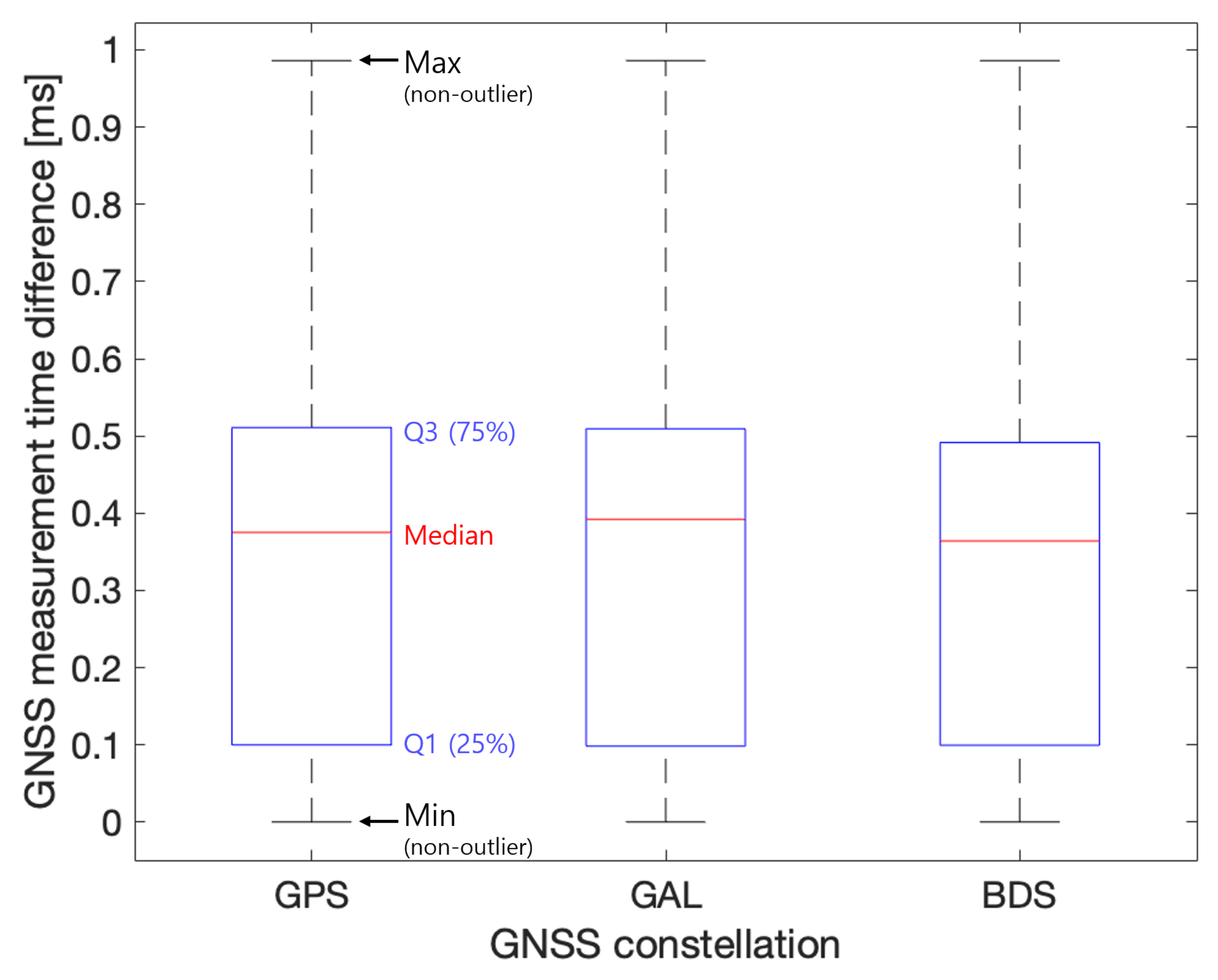
Figure 3.
Box plot of time differences between two GNSS receivers’ (Ublox ZED-F9P) measurements from the flight test data used in this paper. The box plot graphically displays information on the minimum, first quartile, median, third quartile, and maximum values of the given data.
Figure 3.
Box plot of time differences between two GNSS receivers’ (Ublox ZED-F9P) measurements from the flight test data used in this paper. The box plot graphically displays information on the minimum, first quartile, median, third quartile, and maximum values of the given data.

Figure 4.
TDDFC (without cycle slip) values and thresholds derived from the flight test data.

Figure 5.
Miss detection (MD) rates and TDDFC values of (39,30) cycle slips at and bands without noise.
Figure 5.
Miss detection (MD) rates and TDDFC values of (39,30) cycle slips at and bands without noise.

Figure 6.
DACSD (without cycle slip) values and derived thresholds from the flight data. DACSD serves as a complement to the TDDFC method.
Figure 6.
DACSD (without cycle slip) values and derived thresholds from the flight data. DACSD serves as a complement to the TDDFC method.

Figure 7.
TDSFM (without cycle slip) values from the flight data and threshold for cycle slip detection in single-frequency GNSS measurements.
Figure 7.
TDSFM (without cycle slip) values from the flight data and threshold for cycle slip detection in single-frequency GNSS measurements.

Figure 8.
Flowchart for a conventional Kalman filter-based RTK.

Figure 9.
A Kalman filter-based RTK ratio test result with a trend of increasing ratio values.

Figure 10.
Comparison of the Kalman filter gain before and after the inclusion of an AIA state.

Figure 11.
Flowcharts for the proposed dual Kalman filter structure for RTK.

Figure 12.
Ratio values from the flight test #34: main-KF and temp-KF.

Figure 13.
(a) The flight path of four UAVs during the flight tests conducted to collect GNSS data. (b) A hexacopter UAV used for the flight test. The colors of the lines were employed to differentiate the flight paths of each UAV.
Figure 13.
(a) The flight path of four UAVs during the flight tests conducted to collect GNSS data. (b) A hexacopter UAV used for the flight test. The colors of the lines were employed to differentiate the flight paths of each UAV.

Figure 14.
Box plots comparing (a) the percentage of ratio test passes and (b) 3D RMSE with and without GNSS measurements time synchronizations based on the 45 flight test data sets.
Figure 14.
Box plots comparing (a) the percentage of ratio test passes and (b) 3D RMSE with and without GNSS measurements time synchronizations based on the 45 flight test data sets.

Figure 15.
(a) The TDDFC metrics from both static GNSS receivers and flight test data. (b) Number of carrier phase measurements passing the thresholds of the prior art and proposed methods, respectively. The threshold in [36] excludes numerous GNSS data from flight test data (UAVs) compared to the proposed modeled cycle slip detection threshold.


Table 1.
Dual-frequency GNSS signals (,) used in this paper according to each satellite constellation and frequency.
Table 1.
Dual-frequency GNSS signals (,) used in this paper according to each satellite constellation and frequency.
| GPS | Galileo | BeiDou | ||
|---|---|---|---|---|
| Band | L1 | E1 | B1 | |
| Wavelength [m] | 0.19029 | 0.19029 | 0.19204 | |
| Band | L2 | E5b | B2b | |
| Wavelength [m] | 0.24421 | 0.24835 | 0.24835 | |
Table 2.
Examples of cycle slip combinations that result in low TDDFC values [m] without noise.
| TDDFC Values [m] 1 | ||||
|---|---|---|---|---|
| (1,1) | (77,60) | (39,30) | (13,10) | |
| GPS | −0.05392 | 1.7763 | 0.09515 | 0.03172 |
| Galileo | −0.05806 | −0.24835 | −0.02903 | −0.00968 |
| BeiDou | −0.05631 | −0.11392 | 0.03906 | 0.01302 |
1 from the specific cycle slips combination at and (amount of slip in , amount of slip in ).
Table 3.
Thresholds for the absolute values of TDDFC, DACSD, and TDSFM based on flight test data.
| Method | Polynomial Coefficients | |||
|---|---|---|---|---|
| 3rd-Order | 2nd-Order | 1st-Order | Constant | |
| TDDFC [m] | +4.1162 | −1.9358 | −8.2256 | +0.1013 |
| DACSD [cyc] | −1.1586 | +1.8570 | −0.1093 | +7.2164 |
| TDSFM [m/s] | - | - | - | +0.1160 |
Table 4.
A comparison of the RTK performance with conventional KF and dual KF methods (Same cycle slip thresholds were used). Flight test idx 13, highlighted in yellow, showed the largest decrease in RMSE, while the test idx 40, highlighted in gray, demonstrated the largest improvement in passing the ratio test.
| Flight Test Idx | 3D RMSE [cm] (Position Error) | 3D RMSE Reduction Rate [%] | Percentage of Epochs That Passing the Ratio Test [%] | Increase Rate in Passing the Ratio Test [%] | ||
|---|---|---|---|---|---|---|
| Conventional KF | Dual KF | Conventional KF | Dual KF | |||
| 1 | 2.79 | 2.03 | 27.40 | 96.98 | 100.00 | 3.12 |
| 2 | 8.29 | 2.34 | 71.80 | 85.93 | 100.00 | 16.37 |
| 3 | 19.77 | 2.29 | 88.42 | 82.04 | 100.00 | 21.89 |
| 4 | 8.61 | 1.59 | 81.52 | 80.39 | 100.00 | 24.39 |
| 5 | 13.43 | 1.24 | 90.75 | 79.47 | 100.00 | 25.83 |
| 6 | 8.97 | 1.69 | 81.14 | 78.34 | 100.00 | 27.66 |
| 7 | 26.64 | 4.33 | 83.76 | 58.65 | 100.00 | 70.50 |
| 8 | 5.76 | 3.12 | 45.76 | 94.01 | 100.00 | 6.37 |
| 9 | 26.10 | 2.92 | 88.80 | 59.48 | 100.00 | 68.12 |
| 10 | 8.35 | 1.35 | 83.81 | 92.48 | 100.00 | 8.13 |
| 11 | 12.03 | 0.74 | 93.88 | 71.39 | 100.00 | 40.07 |
| 12 | 4.54 | 0.86 | 80.96 | 93.93 | 99.84 | 6.29 |
| 13 | 19.69 | 0.96 | 95.13 | 70.51 | 100.00 | 41.83 |
| 14 | 5.38 | 0.60 | 88.92 | 90.58 | 100.00 | 10.39 |
| 15 | 3.64 | 0.89 | 75.40 | 95.43 | 100.00 | 4.79 |
| 16 | 4.44 | 1.53 | 65.62 | 96.77 | 100.00 | 3.34 |
| 17 | 3.88 | 1.47 | 62.06 | 99.54 | 100.00 | 0.47 |
| 18 | 4.38 | 0.69 | 84.19 | 98.85 | 100.00 | 1.17 |
| 19 | 3.47 | 0.77 | 77.77 | 98.95 | 100.00 | 1.06 |
| 20 | 4.05 | 1.09 | 73.13 | 98.69 | 100.00 | 1.33 |
| 21 | 5.25 | 2.60 | 50.46 | 97.65 | 100.00 | 2.41 |
| 22 | 2.26 | 0.78 | 65.63 | 99.86 | 100.00 | 0.14 |
| 23 | 2.69 | 0.64 | 76.14 | 98.47 | 100.00 | 1.56 |
| 24 | 4.46 | 0.87 | 80.46 | 97.77 | 100.00 | 2.28 |
| 25 | 1.77 | 1.28 | 27.45 | 99.41 | 100.00 | 0.60 |
| 26 | 2.51 | 1.03 | 58.99 | 99.11 | 100.00 | 0.90 |
| 27 | 3.47 | 1.57 | 54.77 | 98.36 | 100.00 | 1.66 |
| 28 | 5.66 | 0.95 | 83.29 | 92.65 | 100.00 | 7.94 |
| 29 | 2.15 | 0.57 | 73.64 | 98.74 | 100.00 | 1.28 |
| 30 | 5.71 | 0.72 | 87.42 | 94.32 | 100.00 | 6.03 |
| 31 | 2.34 | 2.17 | 7.19 | 94.76 | 95.81 | 1.11 |
| 32 | 1.42 | 0.48 | 65.87 | 98.32 | 100.00 | 1.71 |
| 33 | 3.39 | 0.73 | 78.47 | 98.75 | 100.00 | 1.27 |
| 34 | 9.69 | 4.61 | 52.37 | 51.54 | 100.00 | 94.03 |
| 35 | 11.12 | 4.28 | 61.56 | 52.70 | 100.00 | 89.76 |
| 36 | 9.30 | 4.16 | 55.27 | 52.32 | 100.00 | 91.13 |
| 37 | 5.55 | 1.08 | 80.61 | 98.00 | 100.00 | 2.04 |
| 38 | 7.47 | 0.96 | 87.21 | 95.48 | 100.00 | 4.74 |
| 39 | 4.65 | 0.75 | 83.95 | 97.51 | 100.00 | 2.56 |
| 40 | 10.30 | 4.12 | 60.04 | 41.64 | 95.82 | 130.10 |
| 41 | 7.12 | 4.23 | 40.58 | 43.45 | 92.44 | 112.73 |
| 42 | 7.49 | 4.93 | 34.24 | 44.46 | 97.57 | 119.45 |
| 43 | 2.98 | 2.00 | 33.00 | 99.06 | 100.00 | 0.95 |
| 44 | 4.42 | 4.42 | 0.00 | 100.00 | 100.00 | 0.00 |
| 45 | 4.31 | 4.31 | 0.00 | 100.00 | 100.00 | 0.00 |
Disclaimer/Publisher’s Note: The statements, opinions and data contained in all publications are solely those of the individual author(s) and contributor(s) and not of MDPI and/or the editor(s). MDPI and/or the editor(s) disclaim responsibility for any injury to people or property resulting from any ideas, methods, instructions or products referred to in the content. |
© 2024 by the authors. Licensee MDPI, Basel, Switzerland. This article is an open access article distributed under the terms and conditions of the Creative Commons Attribution (CC BY) license (https://creativecommons.org/licenses/by/4.0/).
Share and Cite
MDPI and ACS Style
Shin, Y.; Lee, C.; Kim, E. Enhancing Real-Time Kinematic Relative Positioning for Unmanned Aerial Vehicles. Machines 2024, 12, 202. https://doi.org/10.3390/machines12030202
AMA Style
Shin Y, Lee C, Kim E. Enhancing Real-Time Kinematic Relative Positioning for Unmanned Aerial Vehicles. Machines. 2024; 12(3):202. https://doi.org/10.3390/machines12030202
Chicago/Turabian StyleShin, Yujin, Chanhee Lee, and Euiho Kim. 2024. "Enhancing Real-Time Kinematic Relative Positioning for Unmanned Aerial Vehicles" Machines 12, no. 3: 202. https://doi.org/10.3390/machines12030202
Note that from the first issue of 2016, this journal uses article numbers instead of page numbers. See further details here.