
Anti-Offset Multicoil Underwater Wireless Power Transfer Based on a BP Neural Network
1
School of Marine Electrical Engineering, Dalian Maritime University, Dalian 116026, China
2
Dalian Key Laboratory, Swarm Control and Electrical Technology for Intelligent Ships, Dalian 116026, China
*
Authors to whom correspondence should be addressed.
Machines 2024, 12(4), 275; https://doi.org/10.3390/machines12040275
Submission received: 13 March 2024
/
Revised: 18 April 2024
/
Accepted: 18 April 2024
/
Published: 20 April 2024
(This article belongs to the Section Automation and Control Systems)
Abstract
:Autonomous underwater vehicles (AUVs) are now widely used in both civilian and military applications; however, wireless charging underwater often faces difficulties such as disturbances from ocean currents and errors in device positioning, making proper alignment of the charging devices challenging. Misalignment between the primary and secondary coils can significantly impact the efficiency and power of the wireless charging system energy transfer. To address the issue of misalignment in wireless charging systems, this paper proposes a multiple transfer coil wireless power transfer (MTCWPT) system based on backpropagation (BP) neural network control combined with nonsingular terminal sliding mode control (NTSMC) to enhance further the system robustness and efficiency. To achieve WPT in the ocean, a coil shielding case structure was equipped. In displacement experiments, the proposed multi-transmitting coil system could achieve stable power transfer of 40 W and efficiency of over 78.5% within a displacement range of 8 cm. The system robustness was also validated. This paper presents a new AUV energy supply solution based on MTCWPT. The proposed MTCWPT system can significantly improve the navigation performance of AUVs.
1. Introduction
Underwater wireless charging is an innovative approach designed to provide a continuous energy supply to underwater devices. With the increase in the number of underwater operations and exploration activities, including deep-sea research, underwater pipeline maintenance, and seabed resource exploration, there is a growing demand for an efficient and reliable underwater energy supply [1,2,3]. Wet-mate charging, which requires precise coordination with autonomous underwater vehicles (AUVs) and uses wet connectors that are unreliable, expensive, and have a limited lifespan, is the conventional method [4]. In contrast, underwater wireless charging offers a solution that eliminates the need for physical connections [5,6], significantly enhancing the safety, flexibility, and efficiency of underwater operations.
Wireless charging technology can be divided into three categories based on its working principle: magnetic field coupling, electric field coupling, and electromagnetic radiation.
Inductive power transfer (IPT) technology, whose principle is similar to that of traditional transformers, generates an alternating magnetic field through the action of alternating current on the primary coil. The alternating magnetic field passes through the secondary coil, inducing electromotive force and achieving wireless transmission of electrical energy [7].
The principle of capacitive power transfer (CPT) is similar to that of capacitors. Metal electrode plates are placed on the primary and secondary sides, and an alternating electric field is generated by applying an AC voltage to the primary electrode plate. The secondary metal electrode couples with the primary side through this alternating electric field to achieve wireless transmission of electrical energy [8].
Electromagnetic radiation (ER) wireless charging technology uses electromagnetic waves to transmit electrical energy, converting electrical energy into antenna microwaves. It uses array antennas or other forms of antennas to dissipate and release microwave energy and then converts microwaves back into electrical energy achieving wireless transmission of electrical energy [9].
Compared with IPT, CPT usually considers the use of large-area electrode plates or higher operating frequencies to achieve high-power transmission. However, the greater the operating frequency in seawater, the greater is the eddy current loss. The ER also needs to work in high-frequency mode. The conductivity of the seawater medium will absorb most of the high-frequency electromagnetic wave energy, resulting in low transmission efficiency; therefore, IPT technology is simpler and more practical underwater. Regarding IPT technology, Refs. [10,11,12,13,14,15,16,17,18,19] have mainly conducted further research on coupling devices, compensation networks, power control methods, and other aspects.
However, in the complex environment of underwater wireless charging applications, there may be lateral or longitudinal displacement of the coils between the transmitter and receiver, which reduces the output power and efficiency [10]. Many scholars have conducted extensive research on this issue. The docking system developed by the Woods Hole Institute of Oceanography (WHOI) in Massachusetts, USA, for the Odyssey class underwater robot [11] uses deep-sea mooring equipment supported by surface buoys, as shown in Figure 1a. It provides a protective garage around the underwater robot and does not require additional hardware modifications. This concept is implemented in the REMUS docking stations [12] and the EURODOCKER [13], as shown in Figure 1b. Refs. [11,12] proposed a complete docking method for underwater charging, but the solutions in [11,12] require complex equipment and have high costs.
In 2017, researchers at Zhejiang University in China modified an annular magnetic coupling device placed on an AUV using hollow coils wound around the exterior of the AUV to reduce the weight of the magnetic core of the AUV [3]. However, this configuration makes the internal equipment of the AUV susceptible to electromagnetic interference from the magnetic field, necessitating the installation of aluminum plates within the coils for magnetic shielding. In 2018, researchers at the University of Michigan adopted a segmented design for the annular magnetic coupling device, dividing the secondary side into three identical receiving devices, with the primary side having three identical I-shaped magnetic cores. Three-phase electricity is used for the excitation current in the transmitter, with the excitation current amplitudes and frequencies of the three devices being the same, but shifted by 120° [2]. Based on the bipolar magnetic coupling device, a team from Harbin Institute of Technology proposed an orthogonal coil bipolar magnetic coupling device [14]. In 2019, Hiroyasu Kifune and others from Tokyo University of Marine Science and Technology proposed an optimized coil layout for underwater WPT systems, achieving over 74% transfer efficiency without the need for coil position adjustment [15]. Lee and others studied the effects of high pressure and axial misalignment on the operation of electromagnetic couplers in deep-sea environments by building a 400 W prototype inductive coupler with a pot core [16]. Wang and others designed a loosely coupled wireless system for a 50 kg manned AUV, transmitting 500 W of power with 88% efficiency over a gap distance varying from 6 to 10 mm [17].
However, the various schemes mentioned above are limited to single coil transfer. Single coil wireless power transfer cannot enhance the magnetic field in a certain direction in a directional manner. Therefore, when the secondary coil is offset, a large amount of magnetic leakage is inevitable in single coil wireless power transfer. These magnetic leaks interfere with the operation of AUVs and generate a large amount of eddy current loss in seawater. However, multicoil wireless power transfer can enhance the magnetic field in a certain direction, so it is necessary to conduct research on multicoil wireless energy transfer in the field of underwater wireless power transfer.
This paper introduces a multiple transfer coil WPT (MTCWPT) system with three advantages: resistance to efficiency loss and output reduction due to misalignment, concentration of the magnetic field on the receiving coil to reduce magnetic leakage and eddy current losses, and robustness through nonsingular sliding mode control. The system achieves a transfer power of 40 W within an 80 mm offset range at an input voltage of 25 V, maintaining an efficiency of over 78.5%.
2. Materials and Methods
2.1. Coil Design
2.1.1. The Impact of Seawater on Wireless Power Transfer
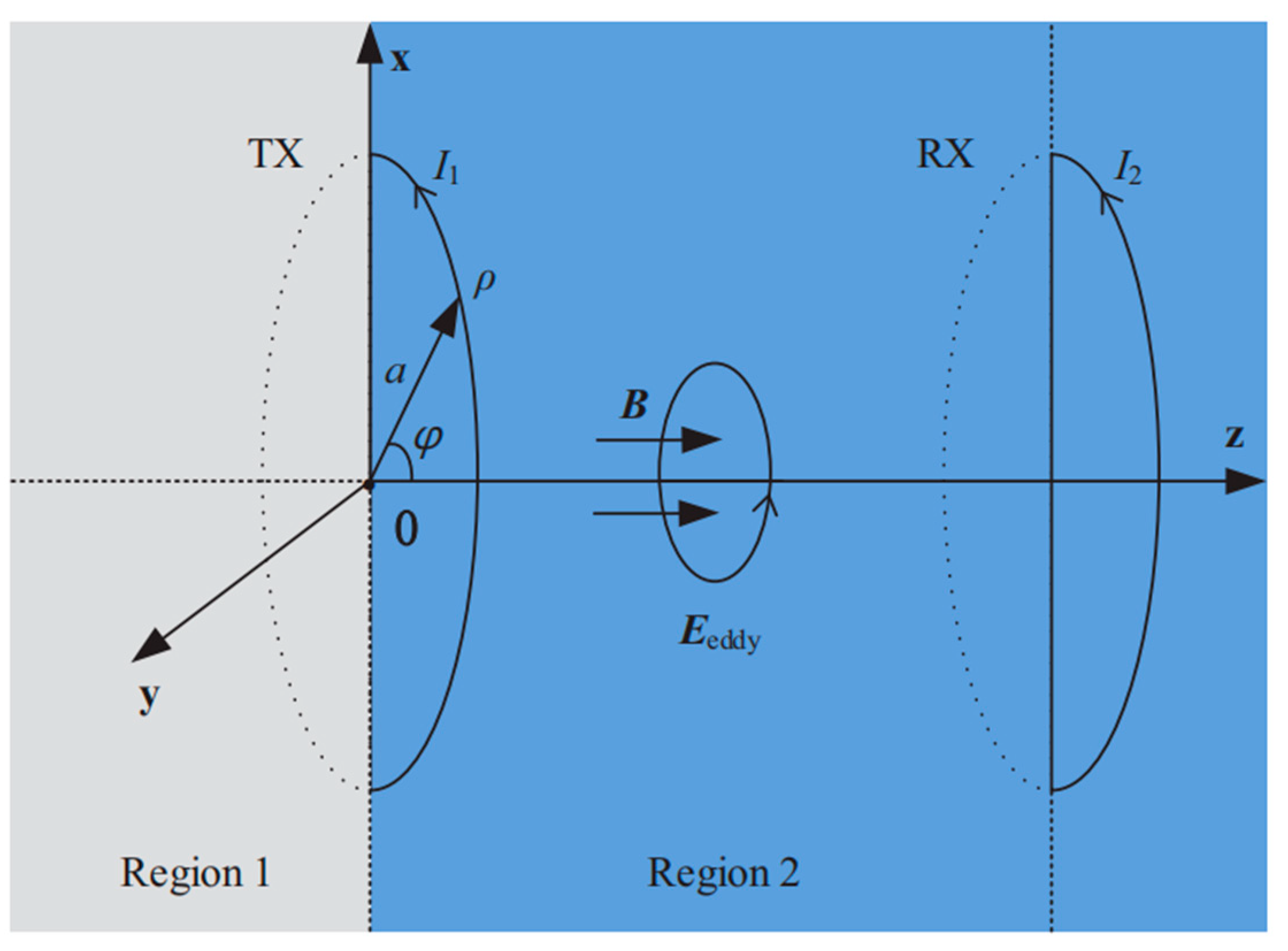
The permeabilities of air and seawater are almost the same, but there is a significant difference in conductivity between air and seawater. The alternating electromagnetic field generated by the high-frequency alternating current in the coil will ultimately result in eddy current losses. Eddy current loss is an important issue in power systems because it can lead to energy waste and equipment heating, thereby affecting the stability and safety of the power system. Figure 2 shows a simplified electric field model for underwater radio energy transfer.
According to Figure 2, the expression for eddy current loss during underwater wireless energy transfer can be listed as follows:
In Equation (1), Peddy is the eddy current loss power, K is a constant, f is the frequency of the electromagnetic field, B is the magnetic induction intensity, δ is the resistivity of seawater, and V is the volume of seawater.
Equation (1) shows that the eddy current loss of underwater wireless energy transfer is mainly affected by the magnetic induction intensity B and the frequency f of the alternating magnetic field. Therefore, the frequency of underwater wireless energy transfer should not be too high. However, a low transfer frequency can also reduce the transfer capacity of wireless energy transfer. After comprehensive consideration, in this article 100 kHz was selected as the frequency for underwater wireless energy transfer.
2.1.2. Single Coil Comparison
The coupling coils used in wireless charging mainly include planar spiral coils and spatial spiral coils. The shape of the spatial spiral coil is cylindrical, and it is installed on the equipment in a vertical structure, occupying a large space. The shape of the planar spiral coil is flat, and it is installed on the equipment in a flat structure, occupying little space. In this article the wireless charging coil structure applied to AUVs was mainly studied. Due to the limited space inside AUVs and underwater AUV charging devices, a planar spiral coil was chosen as the research object. The commonly used planar spiral coils have two structures: circular and rectangular, as shown in Figure 3.
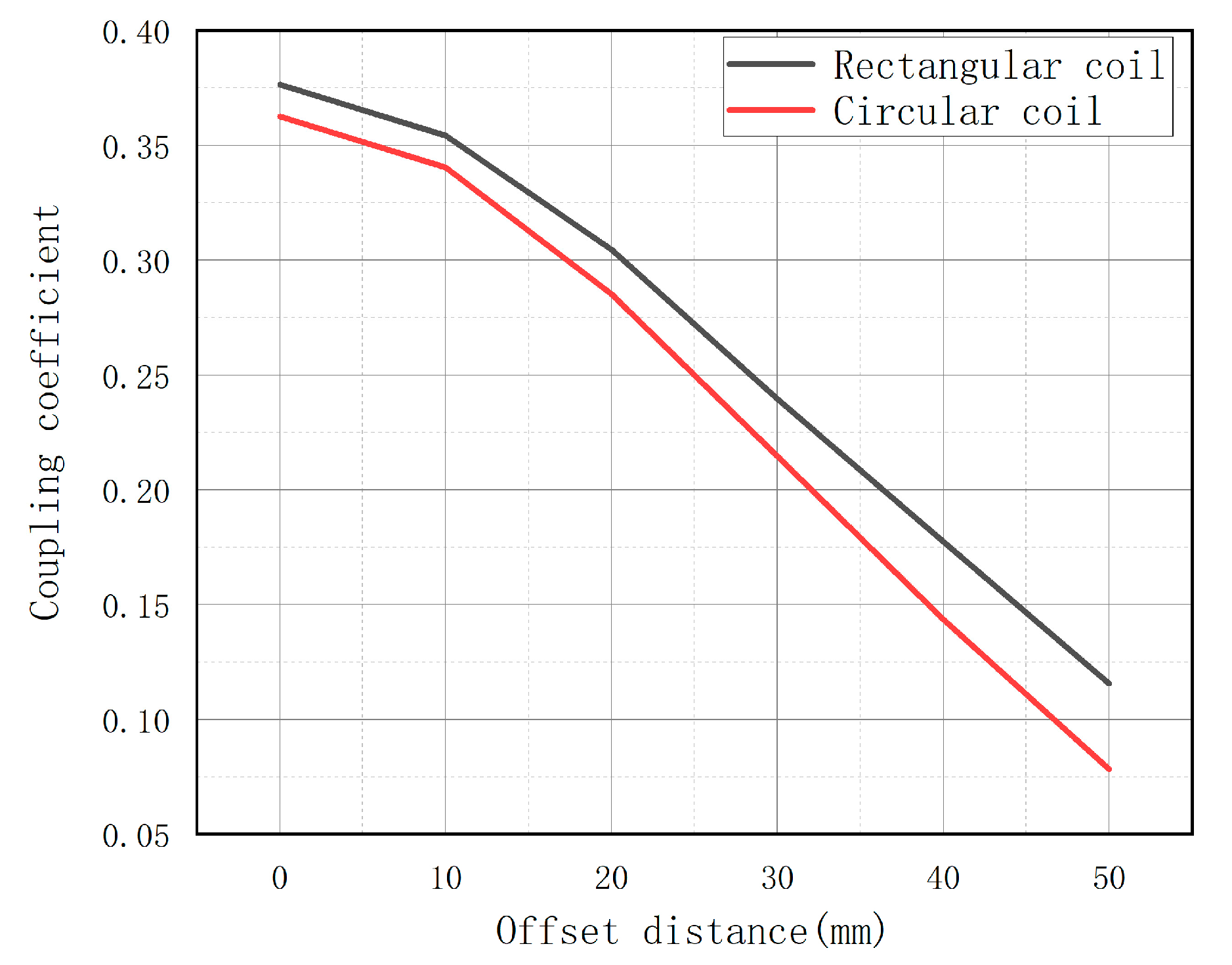
To compare the advantages and disadvantages of circular and rectangular planar coils, 3D simulation models of planar circular coils and rectangular coils were established in the finite element simulation software Maxwell. The simulation model is shown in Figure 4. The parameters of the simulation model in Figure 4 have been provided in Table 1. To avoid errors when comparing the two coils, the sizes of the two coils are set to be consistent when establishing the coil model, and the wire diameter, number of turns, and turn spacing of the two coils are also kept the same. Simulations were conducted under different offset conditions, and the coupling coefficient varied with the offset, as shown in Figure 5.
Through simulation data, it was found that under the same size, the decrease in the coupling coefficient between circular coils with an offset is significantly greater than that between rectangular coils with an offset. The larger the coupling coefficient, the smaller is the magnetic leakage. Underwater wireless energy transfer should consider coil losses, and due to the influence of seawater media, high-frequency alternating magnetic fields will generate much larger eddy currents in seawater than in air, which will result in significant eddy current losses. The smaller the magnetic leakage, the smaller is the eddy current loss generated during wireless energy transfer. At the same size, the eddy current loss generated by transmitting electrical energy between circular coils is significantly greater than that generated by transmitting electrical energy between rectangular coils. Therefore, this article mainly focuses on the study of rectangular coils.
2.1.3. Design of Multi Coil Coupler
When there is a large offset between the primary and secondary sides, the coupling coefficient inevitably decreases, leading to an increase in magnetic leakage and eddy current losses. Currently, there are two main methods to solve this problem: increasing the primary coil and using multi coil transfer. However, increasing the primary coil will inevitably generate more leakage magnetic flux, which will also increase eddy current losses. Therefore, in this study, it was decided to use multiple coils for transfer.
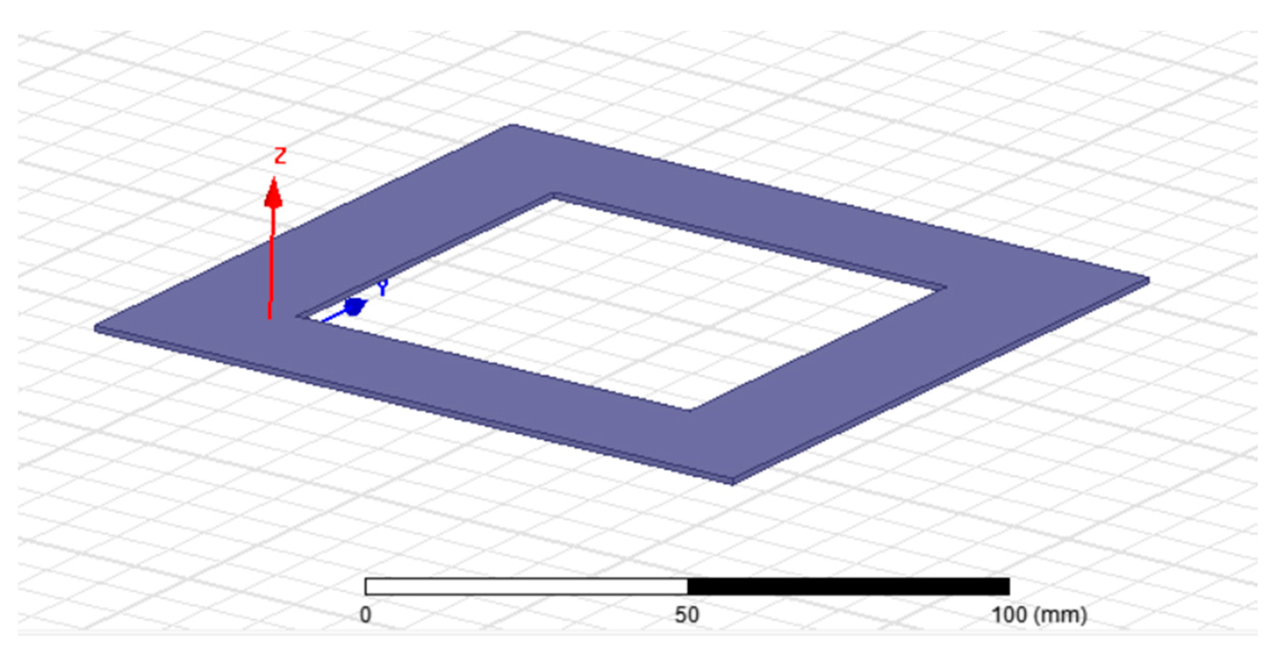
In the wireless charging system designed in this paper, transmitting coils 1, 2, 3, and 4 are all square coils with dimensions of 120 mm × 120 mm, as illustrated in Figure 6.
One critical issue in multicoil wireless charging is that coupling between transmitting coils generates a substantial amount of reactive power. This leads to an increase in the primary-side current, which, in turn, increases coil losses. To decouple the transmitting coils as much as possible, portions of the coils need to overlap. For the ease of subsequent calculation and design, the overlapping portion is fixed at 40 mm. Additionally, to reduce magnetic leakage, ferrite is introduced, as illustrated in Figure 7. The system receiving coil is shown in Figure 8 and the parameters of the transmitting and receiving coils are given in Table 2.
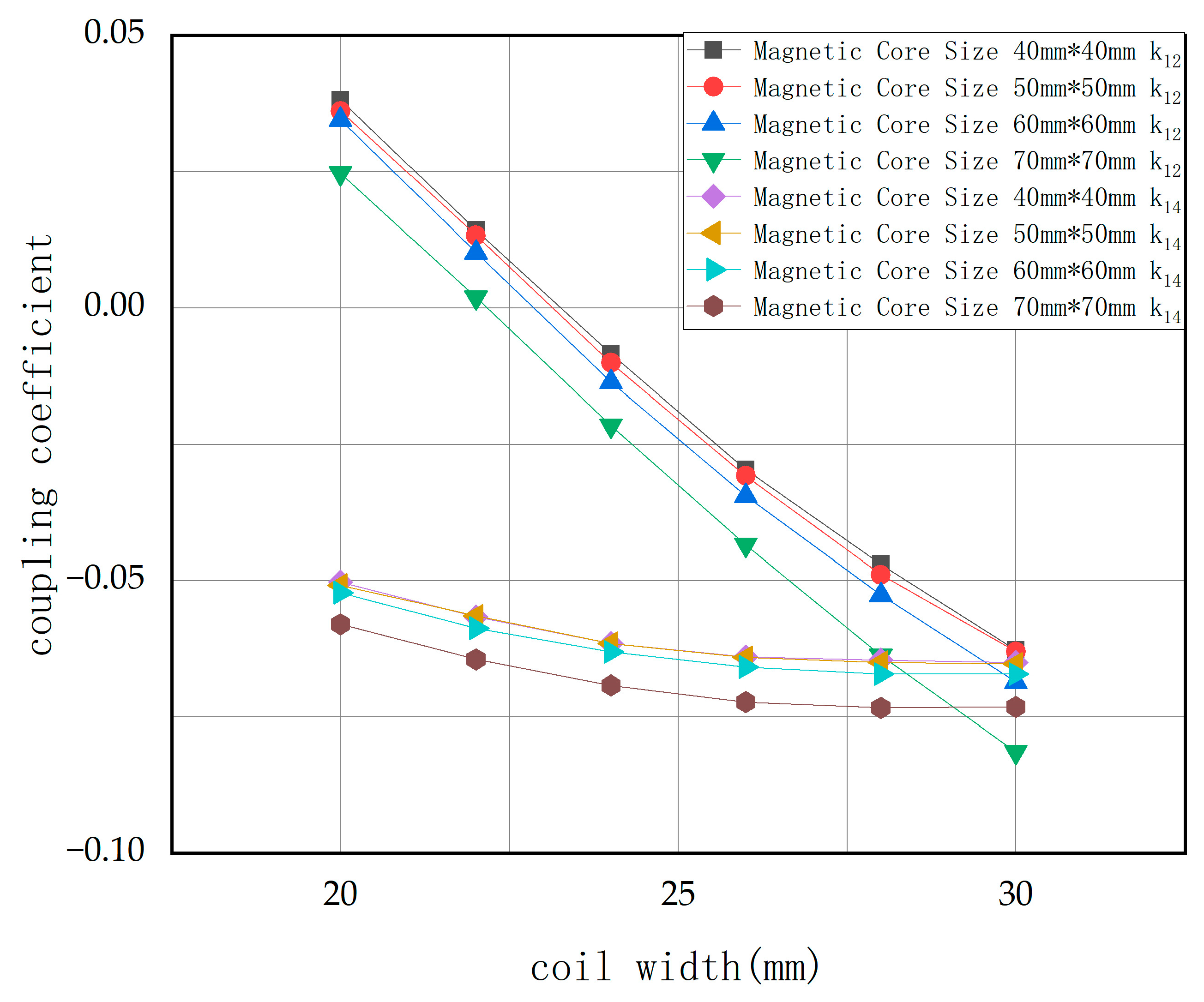
Definitions: is the coupling coefficient between coil 1 and coil 2, is the coupling coefficient between coil 1 and coil 3, is the coupling coefficient between coil 1 and coil 4, is the coupling coefficient between coil 2 and coil 3, is the coupling coefficient between coil 2 and coil 4, and is the coupling coefficient between coil 3 and coil 4. Given that the four coils are symmetrically distributed, the coupling coefficients and . Thus, during the design phase, only decoupling designs for parameters and need to be focused on. Figure 9 shows the trends of changes in coupling coefficients and as the dimensions of the magnetic core and the width of the coils vary.
Figure 9 indicates that the width of the coils has a minimal impact on the coupling coefficient between diagonal coils, while it significantly affects the coupling between adjacent coils. The dimensions of the magnetic core influence both diagonal and adjacent coil coupling; the coupling between diagonal coils decreases with decreasing core size. However, when the core size is reduced to below 50 mm × 50 mm, its effect on the coupling between transmitting coils becomes negligible. Since adjacent coils can be decoupled by adjusting their width, when designing magnetic coupling devices, priority is given to reducing the magnetic core size to decrease the coupling coefficients between diagonal coils. After comprehensive consideration, the designed magnetic coupling device had a coil width of 23 mm and core dimensions of 50 mm × 50 mm.
In Figure 10, M1, M2, M3, and M4 represent the mutual inductance between coils 1, 2, 3, and 4 and the receiving coil. The vertical distance between the transmitting coil and the receiving coil is 20 mm. The magnetic coupling device designed in this article can ensure a large mutual inductance between the transmitting coil and the receiving coil under any offset condition of the secondary side within an offset range of 80 mm in the x and y direction, thus ensuring the anti-offset capability of the system.
2.2. Circuit Design
Figure 11 presents a schematic diagram of the MTCWPT system. The charging structure transfers electrical energy from the four transmitting coils L1, L2, L3, and L4 to the receiving coil. The enclosure of the WPT device is waterproof. Each transmitting coil is powered by an H-bridge inverter circuit, and the direction of the magnetic field is regulated by the depicted control circuit.
Coils 1, 2, 3, and 4 are each coupled with a secondary coil, creating four energy channels, designated energy channels 1, 2, 3, and 4, respectively.
In this study, all the energy channels employ the LCC/S compensation topology, and the overall circuit diagram is illustrated in Figure 12. In Figure 12, M1, M2, M3 and M4 represent the mutual inductances between coils 1, 2, 3, and 4 and the secondary coil.
The transmitter is tuned through an LCC compensation network, while the receiver is tuned through an S compensation network. The circuit parameters are typically designed according to the following equations:
In Equations (2)–(5), ω0 is the resonant frequency of the circuit; L1, L2, L3, and L4 are the inductances of coil 1, coil 2, coil 3, and coil 4, respectively; Lf1, Lf2, Lf3, and Lf4 are the compensation inductances of the primary compensation circuit; C1, C2, C3, C4, C5, C6, C7, and C8 are the compensation capacitances of the primary compensation circuit; LR is the inductance of receiving coil R; C9 is the compensation capacitance of the secondary circuit; P1, P2, P3, and P4 are the input powers of the compensation circuit for coil 1, coil 2, coil 3, and coil 4, respectively; M1, M2, M3, and M4 are the mutual inductances between coil 1 and the secondary coil, coil 2 and the secondary coil, coil 3 and the secondary coil, and coil 4 and the secondary coil, respectively; RLeq is the equivalent resistance of the load and rectifier circuit.
2.3. SV-Based Excitation Method
As shown in Figure 13, we divided the transmitting coil into two groups of BP coils: BP coil BP1 composed of coil 1 and coil 2, and BP coil BP 2 composed of coil 3 and coil 4.
As shown in Figure 14, when secondary coil R is displaced in the y-direction relative to the transmitting coil through spatial vector decomposition, BP1 and BP2 can be considered the stator of a two-phase motor, with the Rreceiver acting as the rotor. The electrical equivalent circuit of the WPT system in Figure 14 shows the receiver misalignment angle derived, based on the receiver longitudinal position relative to the transmitter. In this representation, the receiver misalignment angle is analogous to the rotor position [19].
The reference point for calculating the misalignment angle is the center of the BP1 coil in the y-direction (coinciding with the center of the BP2 coil). This angle is derived from the following equation:
The variable Ry represents the distance from the center of the secondary coil in the y-direction to the center of the transmitting BP1 coil, while b denotes the length of transmission device in the y-direction. Figure 15 depicts the vector diagram of the WPT system.
After converting Figure 14 into a vector graph, Figure 15 can be obtained. The phase shift between BP1 and BP2 is 2π/3 radians. The current vector received by secondary coil R can be obtained through vector addition:
Different values of IBP1 and IBP2 will generate different current vectors I. As shown in Figure 15, the αβ coordinate system is a standing coordinate system. For ease of calculation, we specify the direction of a as the direction of the BP1 current vector. The transmitter current I can be mapped to Iα and Iβ in the αβ plane for further analysis through matrix T:
The dq coordinate system is a rotating coordinate system that is stationary relative to the secondary coil. After components Iα and Iβ are transformed to αβ, the rotation matrix R can be used to orient the system to the receiver reference coordinate system and dq coordinate system, thereby deriving the d-axis component Id and q-axis component Iq of the transmitter current:
By using the inverse T and R transformations, the transmitter current can be represented by its d-axis and q-axis components:
The d-axis current generates a magnetic flux aligned with the receiver, while the q-axis current generates a magnetic flux perpendicular to the receiver. Ideally, a multicoil transmitter should only generate a d-axis current, with the q-axis current being 0, to reduce the magnitude of the transmitter current vector. By setting Iq = 0 and combining Equation (12), the ideal excitation currents IBP1 and IBP2 can be written as functions of θ:
For displacement of secondary coil R in the x-direction relative to the transmitting coil, transmitting coils L1 and L2 can be considered the stator of a two-phase motor, and transmitting coils L3 and L4 can be considered the stator of another two-phase motor, with the receiver acting as the rotor. The current vector required for the secondary coil is generated through vector calculations.
The reference point for calculating the misalignment angle is the center of the BP1 coil in the x-direction. This angle is derived from the following equation:
The variable Rx represents the distance from the center of the secondary coil in the x-direction to the center of the transmitting coil 1, while a denotes the length of transmission device in the x-direction.
2.3.1. BP1 Coil Current Vector Calculation
From the analysis of the equation in the previous section, the current vector that secondary coil R is expected to receive from the BP1 coil is as follows:
BP coil BP1 is controlled similarly to previous analysis. According to Figure 16, the ideal excitation currents I1 and I2 can be written as functions of φ:
2.3.2. BP2 Coil Current Vector Calculation
Similarly, from the analysis in the previous section, the current vector that secondary coil R is expected to receive from the BP2 coil is as follows:
The output voltage of the rectifier bridge UO is as follows:
The output current of the rectifier bridge IO is as follows:
Substituting Equations (15)–(19) into Equation (20) yields the Id required for a fixed output voltage Uout, which is derived as follows:
Substituting Equations (15)–(20) into Equation (21) yields the Id required for a fixed output current Iout as follows:
2.4. Mutual Inductance Measurement and Positioning
2.4.1. Mutual Inductance Measurement
Based on the circuit diagram in Figure 12, a simplified equivalent circuit diagram can be drawn, as shown in Figure 17.
In this design, an LCC-S compensation network is employed. Based on the properties of the LCC-S compensation network, the following can be determined:
Combining Equation (24) with the circuit diagram allows us to derive the expressions for active powers P1, P2, P3, and P4 for energy channels 1, 2, 3, and 4:
To facilitate the calculation during mutual inductance measurement, by design, let Lf1 = Lf2 = Lf3 = Lf4 = Lf. Due to the extremely small internal resistance of the coil relative to the load resistance, it can be neglected during the calculation process; through the two equations above, we can solve for the following:
2.4.2. Position Prediction Based on BP Neural Network
Regarding the issue of the positioning of the primary and secondary coils, many studies are currently being conducted. This paper utilizes four transmitting coils positioned differently coil1, coil2, coil3, and coil4 to replace the four auxiliary coils for coil positioning [20].
As shown in Figure 18, based on the Neumann equation, the expression for mutual inductance between coil A and coil B is as follows:
After converting Equation (27) to the Cartesian coordinate system, we obtain the following:
where (x1, y1, z1) are the coordinates of the center of coil A and (x2, y2, z2) are the coordinates of the center of coil B.
When the relative offset between the positions of the transmitting and receiving coils changes, the mutual inductance between the coils also changes. The coordinates of the receiving coil (x, y, z) can be considered as three variables to be solved, and identification of the mutual inductances for different transmitting coils can enable detection of the relative offset between the coils. However, Equation (27) is clearly a complex nonlinear function.
Artificial neural networks achieve structured combinations of relatively simple mathematical expressions to produce more flexible and descriptive expressions describing the input-output relationships in specific processes. To overcome the limitations of traditional problem analysis due to complex quantification, backpropagation (BP) neural networks have been widely used for data prediction, pattern recognition, fault classification, etc. Therefore, a BP neural network was used for the designed wireless charging system to predict the secondary-side position.
The basic unit of the BP neural network is neurons. The general model of neurons is shown in Figure 19, where the commonly used activation function is the sigmoid function. Its characteristic is that the function itself and its derivatives are continuous, making it very convenient to handle:
The output of a single neuron is as follows:
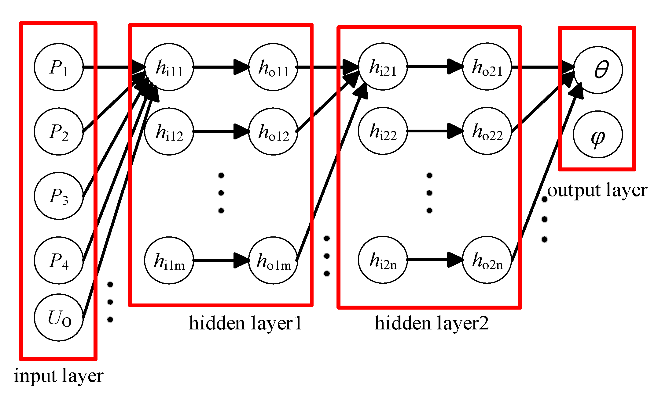
A neural network is a network formed by connecting multiple neurons together according to certain rules, as shown in Figure 20. A neural network consists of an input layer, a hidden layer (middle layer), and an output layer. The number of neurons in the input layer is the same as the dimension of the input data, the number of neurons in the output layer is the same as the number of data to be fitted, and the number of neurons in the hidden layer needs to be set by the designer according to certain rules and objectives. Before the emergence of deep learning, the number of hidden layers was usually one, which means that the commonly used neural network was a three-layer network. Equation (28) is a nonlinear function. To reduce the computational complexity of the controller, this paper adopted a BP neural network with two hidden layers.
The specific learning process of the BP neural network is shown in Figure 21.
Equation (25) shows that the mutual inductances between the four transmitting coils and the receiving coil can be obtained from the input voltage, input power, and output voltage. And the position of the receiving coil relative to the transmitting coil can be obtained from the mutual inductances between the four transmitting coils and the receiving coil. The input voltage and input power can be directly obtained from the primary signal acquisition circuit, and the output voltage can be acquired by the secondary signal acquisition circuit and transmitted to the primary side via wireless communication. The use of a BP neural network to train the input voltage, input power, output voltage, and corresponding secondary coil position can enable the prediction of the secondary coil position.
2.5. Nonsingular Terminal Sliding Mode Control
In traditional control technologies, challenges such as significant vibrations and slow response times exist. To further enhance the system robustness, this paper combines phase-shift control with nonsingular terminal sliding mode control (NTSMC) and neural networks [21].
First, according to Figure 12, we establish the equivalent topological circuit equations for the LCC-S system:
The expected output voltage of the system is set as . Letting the control variables , , and , the state-space equations for the LCC-S system can be described as follows:
The proposed sliding mode approach law is designed as below:
To eliminate vibrations as much as possible, SMC needs to satisfy the following conditions: Condition 1: rapid convergence to the sliding surface; Condition 2: a finite time to reach the sliding surface; and Condition 3: the velocity is zero when reaching the switching surface, i.e., the following:
Setting the initial value of s(t) as s(0), integrating Equation (33), and setting s = 0, we can solve for the following:
when t = τ, Condition 2 and Condition 3 are satisfied. Since 0 < α < 1, Condition 1 is also satisfied.
The system sliding surface is chosen as follows:
where β, p, and q are the equivalent control coefficients. The selection of these coefficients must meet the existence conditions of SMC, which are derived using Lyapunov’s second method as follows:
By substituting (32) and (35) into (37), we find that the necessary and sufficient condition for the existence of a sliding mode on the switching surface is that the equivalent control satisfies the following equation:
By introducing the approach law (32), we obtain the following:
As long as is satisfied, the approach law meets the conditions for the existence and global reaching of the sliding mode.
The actual control law of the sliding mode controller is as follows:
After combining nonsingular SMC with the BP neural network, the control rate equation for the four energy channels is as below:
The input voltages of the four energy channels are as follows:
3. Results
3.1. Construction of Simulation Models and Experimental Platforms
In order to further verify the theory in the above analysis, we used ANSYS to build the coil model as shown in Figure 22 and Simulink to build the circuit model as shown in Figure 23, then conducted simulation. Reference Table 2 for the coil simulation model. The simulation parameters of Simulink are shown in Table 3.
The experimental prototype constructed in the laboratory is shown in Figure 24. The coupling conditions for the experiment are not fixed but are varied. The transmitting coil is stationary, while the receiving coil can move in both the x-direction and y-direction. The measurement instruments used in the experiment were a RIGOL MSO5104 oscilloscope, a CYBERTEK P1300 isolated voltage probe, and a CYBERTEK HCP8030D current probe. The controllers used in the experiment were STM32F103ZET6 and STM32F103RCT6. The MOSFET model for the inverter bridge is an IRF540N. The coil used in the experiment was wound with 120 × 0.1 mm silk wrapped wire, and the capacitors were all high-temperature resistant metal film capacitors. The actual circuit parameters measured are shown in Table 4.
3.2. BP Neural Network Training
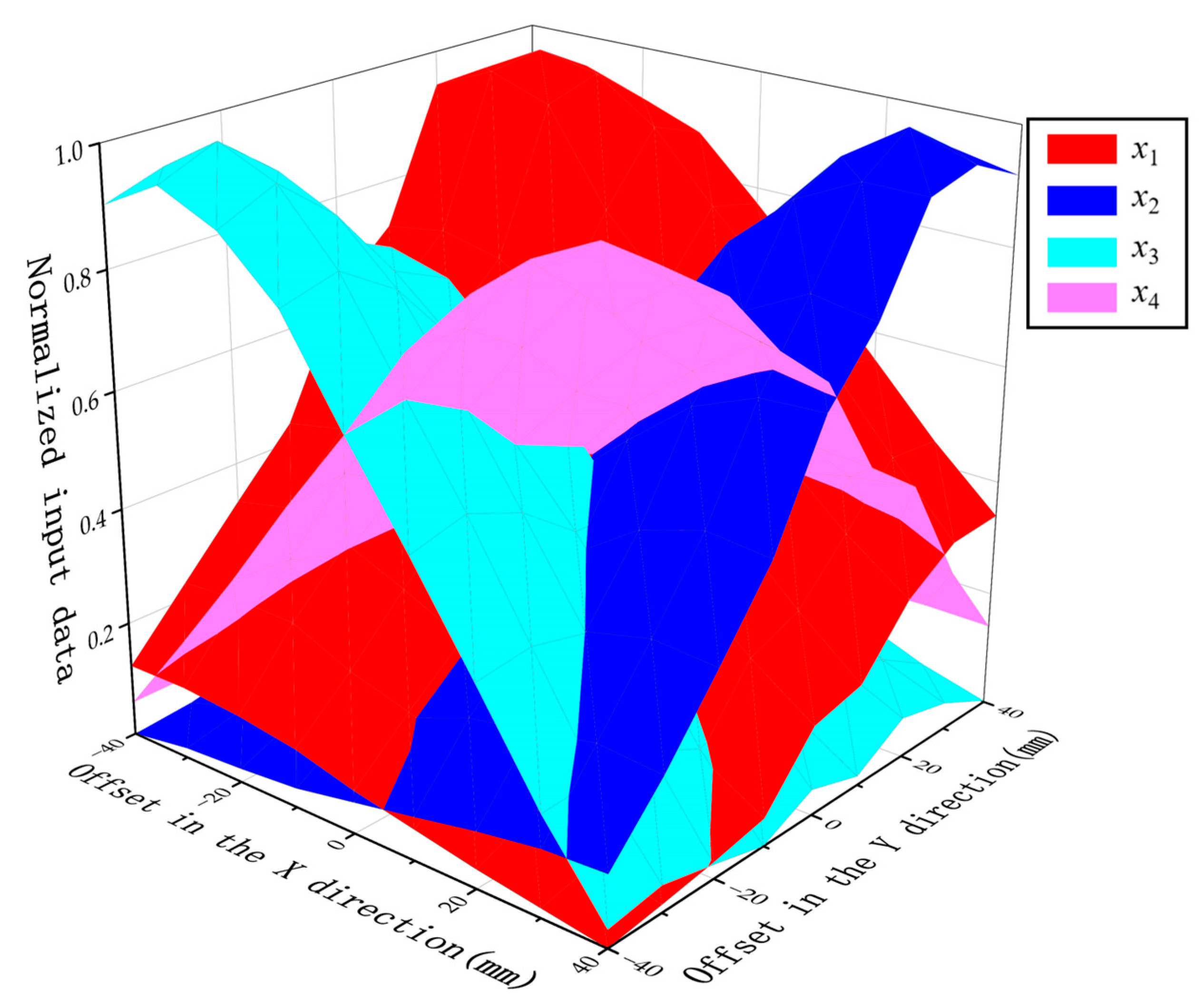
Based on the analysis in Section 2.4.2, we know that the position of the secondary coil can be determined by the mutual inductance between the four coils with different center positions and the secondary coil. The inputs of the four neural networks are denoted as x1, x2, x3, and x4
The output of the BP neural network is set to the offset of the secondary coil in the x direction and the offset of the secondary coil in the y direction. The following dataset is obtained after measuring the power supply through actual circuit connections. Partial data are shown in Figure 25. The variation trend of x1, x2, x3, and x4 calculated based on actual data with the offset in Figure 25 is very close to the variation trend of M1, M2, M3, and M4 in Figure 10. Consider x1, x2, x3, and x4 as functions associated with specific positions, each linearly independent from the others. With the coordinates (x,y) of the receiving coil as unknowns, it is possible to establish a system comprising four linearly independent equations in two variables. This setup allows us to demonstrate that the coordinates (x,y) can be uniquely determined.
After being trained with the actual measured input current and voltage of the transmitting coil and the output voltage of the receiving coil, the training objective is to minimize the normalized mean square error (NMSE) between the predicted position of the receiving coil and the actual position of the coil. The equation for calculating the NMSE is as follows:
In Equation (44), m is the number of samples, is the position of the secondary coil predicted by the BP neural network in the x direction, x is the actual position of the secondary coil in the x direction, is the position of the secondary coil predicted by the BP neural network in the x direction, and y is the actual position of the secondary coil in the y direction.
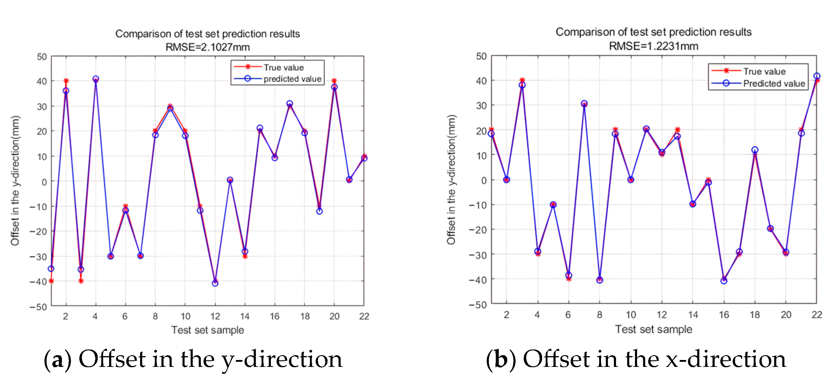
The BP neural network can achieve a position prediction accuracy of 99.6% for the receiving coil. The results of the data training for the BP neural network are shown in Figure 26 and Figure 27. The round of neural networks in Figure 26 refers to the learning process completed by the neural network on the data in Figure 25, as shown in Figure 20. The RMSE in Figure 27a,b is the root mean square error. The specific equation for the RMSE in Figure 27a RMSEy and the RMSE in Figure 27b RMSEx is as follows:
3.3. Magnetic Field Simulation
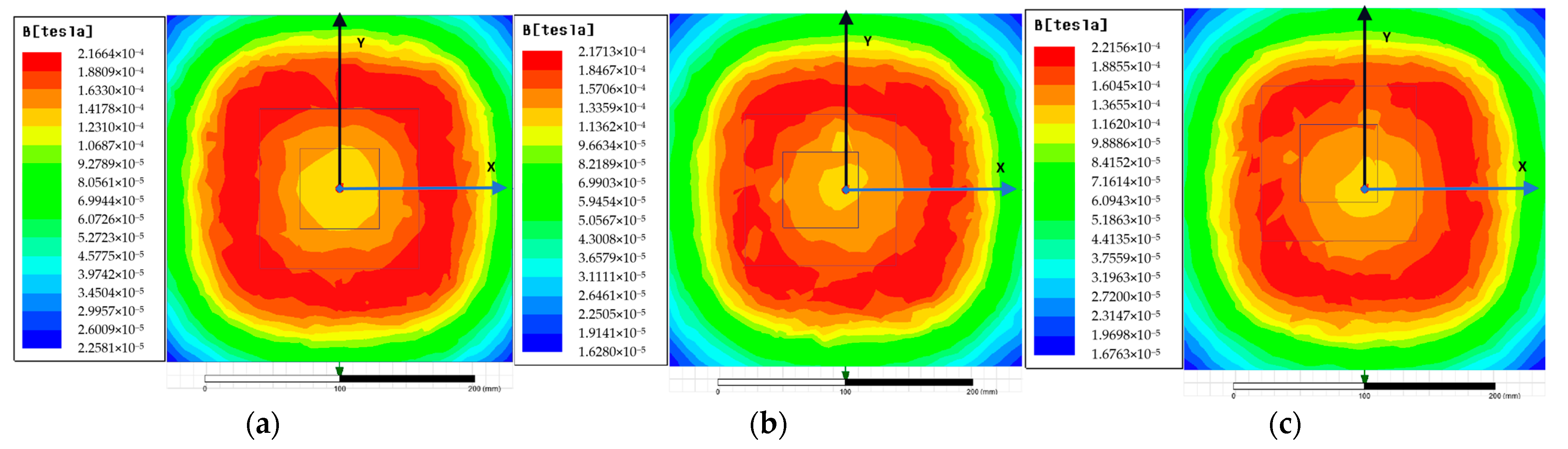
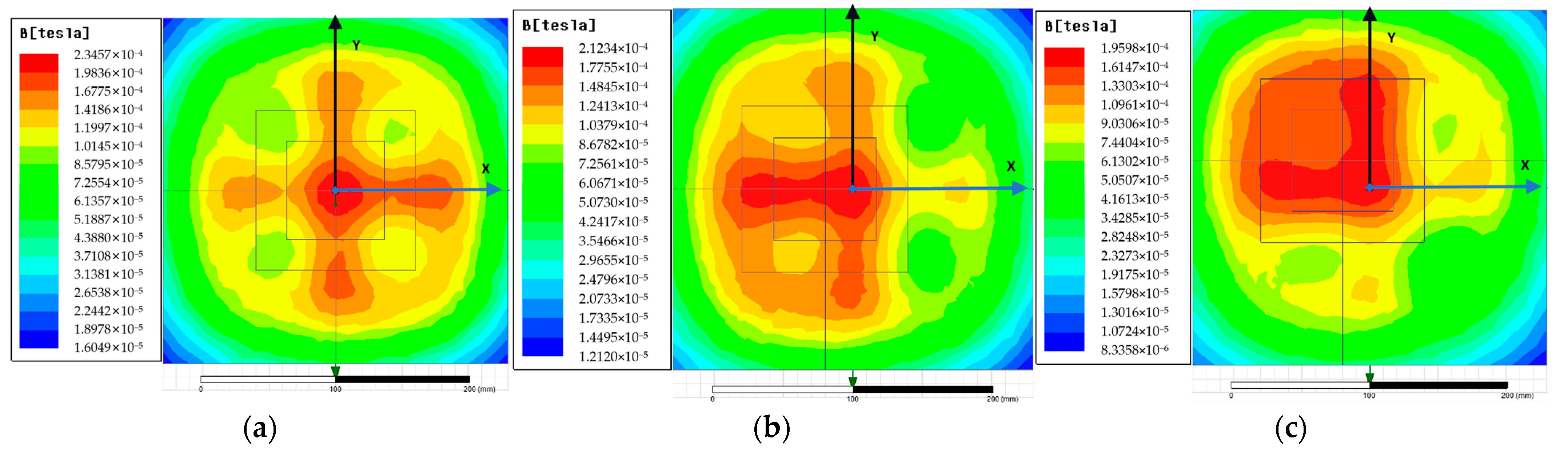
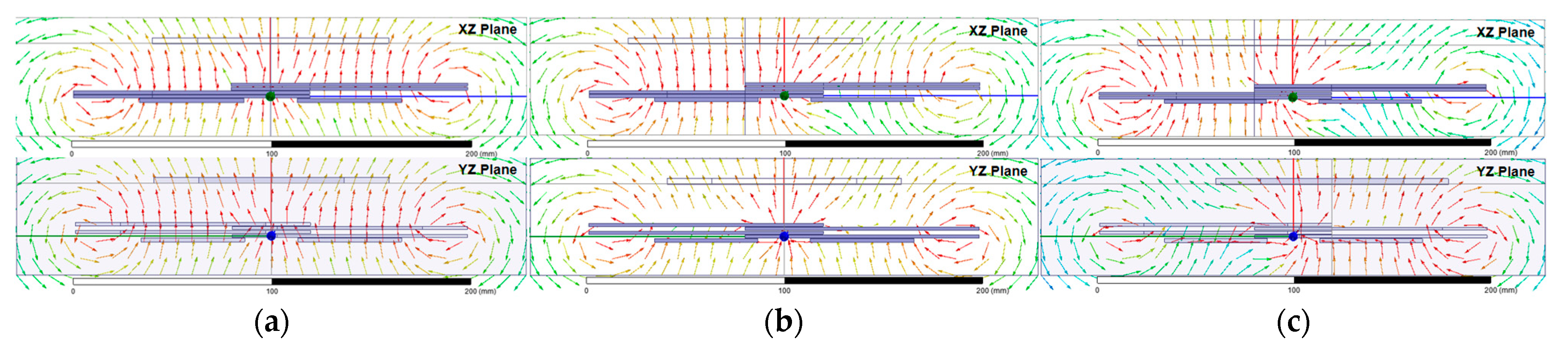
In Maxwell, simulation models for the proposed multicoil were developed. To better demonstrate the advantages of multicoil transfer, we built a single coil transfer model of the same size (200 mm × 200 mm) and the same coil width (23 mm) as a control. The simulation facilitated a comparison and validation of the magnetic field distributions resulting from the lateral misalignment and longitudinal displacement of the coils. In these simulations, the secondary-side coils each received a voltage of 20 V. The distribution of magnetic field intensity and magnetic field vector obtained under different offset conditions are shown in Figure 28, Figure 29 and Figure 30.
The simulation results reveal that in the traditional single-coil coupling energy transfer process, the single coil generates a magnetic field that scatters away from the center of the coil. In contrast, the multicoil transfer structure can adjust the magnetic field in response to the movement of the secondary-side coil, concentrating the magnetic field near the center of the receiving coil. A key aspect of underwater WPT is minimizing the leakage of magnetic fields from the WPT device, thereby reducing eddy current losses in seawater. The diagrams clearly show that the magnetic leakage of the multicoil transfer structure is significantly less than that of the single-coil transfer structure, indicating that the proposed system has advantages in magnetic field coupling.
3.4. Experimental Verification
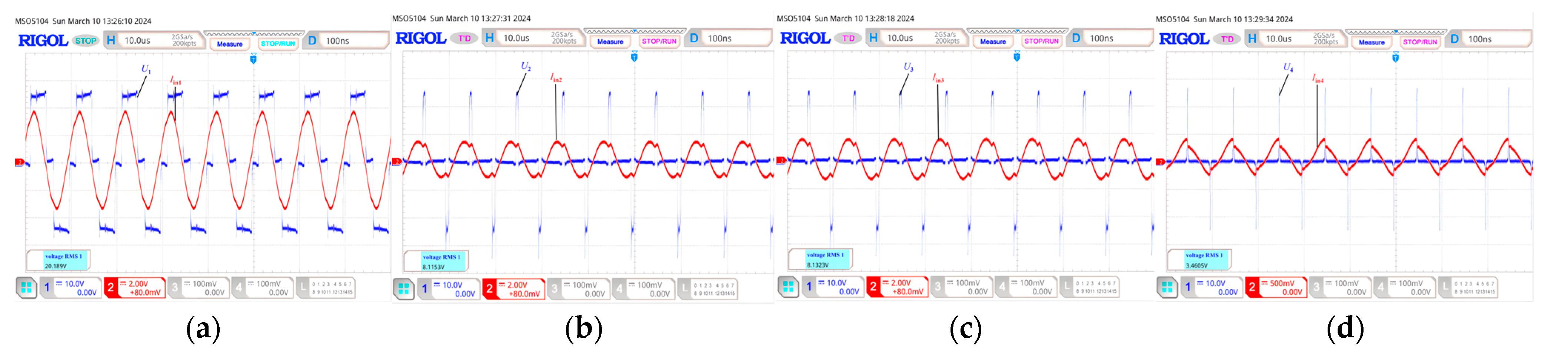
Experiments were conducted to validate both traditional WPT and the proposed system, with the input voltage set at 25 V, the output voltage set at 20 V, and the transmitter and receiver separated by 20 mm. Figure 31 displays the voltage and current waveforms of the secondary-side coil without any offset during WPT, while Figure 32 shows the voltage and current waveforms when the secondary-side coil is offset by 2 cm in both the x- and y-directions during WPT. A 1:1 probe was used for the current measurements. From Figure 31 and Figure 32, it can be seen that when the secondary coil undergoes displacement, the inverter bridge allocates electrical energy as envisioned in Section 2.3, directionally adjusts the magnetic field, and verifies the control effect of the BP neural network.
Figure 33 illustrates the output efficiency related to coil misalignment at a transfer power of 40 W. Figure 33 shows that the MTCWPT equipment maintains a relatively high transfer efficiency within a 4 cm offset range, and the experimental results are slightly lower than the simulation results. This is because the experiment did not use the ideal device as in the simulation, and the inverter bridge, wire, and capacitor in the experiment generated heat and loss. Moreover, in the experiment, the compensation circuit cannot achieve the same resonant state as in the simulation.
The NTSMC parameters obtained from tuning are p/q = 1.04, β = 44,789, α = 0.01, and kt = 3,075,700,000. The NTSMC step response curve obtained from the experiment is shown in Figure 34. The experiment was designed with an x-direction offset varying from 0 to 10 mm and a y-direction offset from 0 to 10 mm. The output voltage waveform of the NTSMC offset change experiment is displayed in Figure 34. The calculation formula for the high values VH in Figure 34 and Figure 34 is shown in Equation (47).
In Equation (47), Vmin is the minimum value of the waveform, and Vmax is the maximum value of the waveform.
Figure 34 shows that the system using SMC reduces the rise time to only 15 ms, with no overshoot during the rising process. Figure 35 shows the variation of load voltage during the coupling process of the system from positive to offset of about 1.5 cm. It can be seen that the output voltage of the system quickly reaches a stable state after a brief fluctuation, and the process only lasts for 6 ms, and during the voltage fluctuation period, there is only an 11.24% reduction in the voltage, demonstrating the strong robustness of the system and having obvious advantages for its application in complex underwater environments.
Figure 36 shows the voltage output waveform when the secondary coil vibrates. Figure 36a shows the voltage output waveform when a small vibration occurs, with a vibration range of 0 mm to 15 mm and a vibration speed of approximately 1500 mm/s. Figure 36a shows that when the secondary coil vibrates, the output voltage fluctuates very little or even not at all, with a maximum fluctuation of approximately 6%. When the vibration ends, the voltage immediately stabilizes. Figure 36b shows the voltage output waveform when a large vibration occurs, with a vibration range of 0 mm to 30 mm and a vibration speed of approximately 3000 mm/s. Figure 36b shows that when the secondary coil experiences a large vibration, the maximum fluctuation in the output voltage is approximately 15%. When the vibration ends, the voltage immediately stabilizes, and the output voltage is still within a controllable range.
4. Discussion
From the results, with an input DC voltage of 25 V, the WPT system we constructed can maintain a stable power output of 40 W and an efficiency of over 78.5%, while the step response time of the system is 15 ms. When a small offset occurs, the system needs only 6 ms to stabilize, and the robustness of the system was verified through experiments. When the secondary coil undergoes slight vibration, the output has little effect. Moreover, in practical applications, the standard input DC voltage on AUVs can achieve kilowatt-level charging power. Although magnetic leakage is of significant practical importance in real underwater robots, the proposed multicoil wireless charging structure can effectively prevent leakage. However, the design of this article is limited to only the control aspect, and there has not been in-depth research on coil design. In fact, coil resistance is still a major issue in the process of wireless energy transfer [22], and future research will focus on coil design to reduce copper loss during wireless energy transfer.
5. Conclusions
This article introduces a new charging method that combines BP neural networks with SMC. Through mathematical modelling, magnetic field modelling, and experimental verification, the feasibility of this method was demonstrated. The research shows that multicoil wireless charging enhances the mutual inductance of traditional WPT systems, improving their stability and efficiency. The proposed charging system also exhibited significant stability advantages in lateral misalignment experiments, achieving stable and effective WPT within an 8 cm displacement range.
Author Contributions
Conceptualization, Y.F. and H.T.; methodology, Y.F.; software, H.T.; validation, Y.F., H.T. and J.L.; formal analysis, H.T.; investigation, H.T.; resources, Y.F.; data curation, J.L.; writing—original draft preparation, H.T.; writing—review and editing, Y.F.; visualization, H.T. and J.L.; supervision, Z.P.; project administration, Y.F.; funding acquisition, Y.F. All authors have read and agreed to the published version of the manuscript.
Funding
This research was funded by the Fundamental Research Funds for the Central Universities, grant number 3132023112, and the Spring Sunshine Plan Research Project of the Ministry of Education of China, grant number HZKY20220410.
Data Availability Statement
Data are contained within the article.
Conflicts of Interest
The authors declare no conflicts of interest.
References
- Kan, T.; Zhang, Y.; Yan, Z.; Mercier, P.P.; Mi, C.C. A rotation-resilient wireless charging system for lightweight autonomous underwater vehicles. IEEE Trans. Veh. Technol. 2018, 67, 6935–6942. [Google Scholar] [CrossRef]
- Kan, T.; Mai, R.; Mercier, P.P.; Mi, C.C. Design and Analysis of a Three-Phase Wireless Charging System for Lightweight Autonomous Underwater Vehicles. IEEE Trans. Power Electron. 2017, 33, 6622–6632. [Google Scholar] [CrossRef]
- Lin, M.; Li, D.; Yang, C. Design of an ICPT system for battery charging applied to underwater docking systems. Ocean Eng. 2017, 145, 373–381. [Google Scholar] [CrossRef]
- Covic, G.A.; Boys, J.T. Modern Trends in Inductive Power Transfer for Transportation Applications. IEEE J. Emerg. Sel. Top. Power Electron. 2013, 1, 28–41. [Google Scholar] [CrossRef]
- Teeneti, C.R.; Truscott, T.T.; Beal, D.N.; Pantic, Z. Review of wireless charging systems for autonomous underwater vehicles. IEEE J. Ocean. Eng. 2019, 46, 68–87. [Google Scholar] [CrossRef]
- Huda, S.M.A.; Arafat, M.Y.; Moh, S. Wireless Power Transfer in Wirelessly Powered Sensor Networks: A Review of Recent Progress. Sensors 2022, 22, 2952. [Google Scholar] [CrossRef] [PubMed]
- Hui, S.Y.R.; Zhong, W.; Lee, C.K. A Critical Review of Recent Progress in Mid-Range Wireless Power Transfer. IEEE Trans. Power Electron. 2014, 29, 4500–4511. [Google Scholar] [CrossRef]
- Dai, J.; Ludois, D.C. A Survey of Wireless Power Transfer and a Critical Comparison of Inductive and Capacitive Coupling for Small Gap Applications. IEEE Trans. Power Electron. 2015, 30, 6017–6029. [Google Scholar] [CrossRef]
- Koohestani, M.; Zhadobov, M.; Ettorre, M. Design Methodology of a Printed WPT System for HF-Band Mid-Range Applications Considering Human Safety Regulations. IEEE Trans. Microw. Theory Tech. 2016, 65, 270–279. [Google Scholar] [CrossRef]
- Zhang, Z.; Zhang, B. Omnidirectional and Efficient Wireless Power Transfer System for Logistic Robots. IEEE Access 2020, 8, 13683–13693. [Google Scholar] [CrossRef]
- Singh, H.; Bellingham, J.; Hover, F.; Lemer, S.; Moran, B.; von der Heydt, K.; Yoerger, D. Docking for an autonomous ocean sampling network. IEEE J. Ocean. Eng. 2001, 26, 498–514. [Google Scholar] [CrossRef]
- Brighenti, A.; Zugno, L.; Mattiuzzo, F.; Sperandio, A. EURODOCKER-a universal docking-downloading recharging system for AUVs: Conceptual design results. In Proceedings of the IEEE Oceanic Engineering Society, OCEANS’98, Nice, France, 28 September–1 October 1998; Volume 3, pp. 1463–1467. [Google Scholar]
- Fukasawa, T.; Noguchi, T.; Kawasaki, T.; Baino, M. “MARINE BIRD”, a new experimental AUV with underwater docking and recharging system. In Proceedings of the Oceans 2003. Celebrating the Past … Teaming Toward the Future (IEEE Cat. No. 03CH37492), San Diego, CA, USA, 22–26 September 2003. [Google Scholar]
- Cai, C.; Wu, S.; Zhang, Z.; Jiang, L.; Yang, S. Development of a Fit-to-Surface and Lightweight Magnetic Coupler for Autonomous Underwater Vehicle Wireless Charging Systems. IEEE Trans. Power Electron. 2021, 36, 9927–9940. [Google Scholar] [CrossRef]
- Sato, N.; Kifune, H.; Komeda, S. A coil layout of wireless power transfer systems based on multicoil arrangement for underwater vehicles. Electr. Eng. Jpn. 2019, 207, 38–48. [Google Scholar] [CrossRef]
- Li, Z.; Li, D.; Lin, L.; Chen, Y. Design considerations for electromagnetic couplers in contactless power transfer systems for deep-sea applications. J. Zhejiang Univ. Sci. C. 2010, 11, 824–834. [Google Scholar] [CrossRef]
- Wang, S.-L.; Song, B.-W.; Duan, G.-L.; Du, X.-Z. Automatic wireless power supply system to autonomous underwater vehicles by means of electromagnetic coupler. J. Shanghai Jiaotong Univ. 2014, 19, 110–114. [Google Scholar] [CrossRef]
- Yan, Z.; Zhang, Y.; Kan, T.; Lu, F.; Zhang, K.; Song, B.; Mi, C. Eddy Current Loss Analysis of Underwater Wireless Power Transfer System. In Proceedings of the 2018 IEEE Transportation Electrification Conference and Expo (ITEC), Long Beach, CA, USA, 13–15 June 2018; pp. 881–884. [Google Scholar]
- Pathmanathan, M.; Nie, S.; Yakop, N.; Lehn, P.W. Space-Vector Based Excitation of a Bipolar Transmitter for Wireless Power Transfer Applications. IEEE Trans. Ind. Electron. 2020, 68, 12524–12534. [Google Scholar] [CrossRef]
- Gao, Y.; Duan, C.; Oliveira, A.A.; Ginart, A.; Farley, K.B.; Tse, Z.T.H. 3-D Coil Positioning Based on Magnetic Sensing for Wireless EV Charging. IEEE Trans. Transp. Electrif. 2017, 3, 578–588. [Google Scholar] [CrossRef]
- Robles, J.; Sotelo, F.; Chavez, J. Robust Nonsingular Terminal Sliding Mode Control with Constant Frequency for DC/DC Boost Converters. In Proceedings of the 2020 IEEE 21st Workshop on Control and Modeling for Power Electronics (COMPEL), Aalborg, Denmark, 9–12 November 2020; pp. 1–5. [Google Scholar]
- Stankiewicz, J.M. Estimation of the Influence of the Coil Resistance on the Power and Efficiency of the WPT System. Energies 2023, 16, 6210. [Google Scholar] [CrossRef]
Figure 1.
Underwater wireless energy transfer case. (a) Dock mooring system (b) REMUS docking station.
Figure 1.
Underwater wireless energy transfer case. (a) Dock mooring system (b) REMUS docking station.

Figure 2.
The simplified calculation model [18].
Figure 2.
The simplified calculation model [18].

Figure 3.
The planar spiral coils. (a) Circular planar spiral coil (b) Rectangle planar spiral coil.
Figure 3.
The planar spiral coils. (a) Circular planar spiral coil (b) Rectangle planar spiral coil.

Figure 4.
Simulation model of the planar spiral coils. (a) Simulation model of rectangle planar spiral coil (b) Simulation model of circular planar spiral coil.
Figure 4.
Simulation model of the planar spiral coils. (a) Simulation model of rectangle planar spiral coil (b) Simulation model of circular planar spiral coil.

Figure 5.
The variation in the coupling coefficient with offset.

Figure 6.
Single transmitting coil.

Figure 7.
Transmitting coil device.

Figure 8.
Receiving coil.

Figure 9.
Variation trends of coupling coefficients k12 and k14 with the coil parameters.

Figure 10.
The variation of coupling coefficient between transmitting coil and receiving coil with offset.
Figure 10.
The variation of coupling coefficient between transmitting coil and receiving coil with offset.

Figure 11.
MTCWPT system circuit diagram.

Figure 12.
MTCWPT overall circuit diagram.

Figure 13.
Coil grouping diagram.

Figure 14.
Representation of BP1 and BP2 transmitter as the stator and the receiver coil as the rotor of a rotating electrical machine, with receiver misalignment analogous to rotor position θ.
Figure 14.
Representation of BP1 and BP2 transmitter as the stator and the receiver coil as the rotor of a rotating electrical machine, with receiver misalignment analogous to rotor position θ.

Figure 15.
BP coil electric current vector diagram.

Figure 16.
BP1 coil electric current vector diagram.

Figure 17.
Equivalent circuit diagram.

Figure 18.
Calculation diagram for two square coils.

Figure 19.
Single neuron model.

Figure 20.
BP neural network structure diagram.

Figure 21.
BP neural network learning process.

Figure 22.
Underwater magnetic coupling simulation model.

Figure 23.
Circuit simulation model.

Figure 24.
Laboratory prototype and laboratory equipment.

Figure 25.
Training data for neural networks.

Figure 26.
Performance of BP neural network after training.

Figure 27.
Comparison of the prediction results based on the training set.

Figure 28.
Magnetic field distribution diagrams of a single-coil transfer structure. (a) Without offset. (b) Offset by −20 mm in the x-direction. (c) Offset by −20 mm in the x-direction and 20 mm in the y-direction.
Figure 28.
Magnetic field distribution diagrams of a single-coil transfer structure. (a) Without offset. (b) Offset by −20 mm in the x-direction. (c) Offset by −20 mm in the x-direction and 20 mm in the y-direction.

Figure 29.
Magnetic field distribution diagram of the multicoil transfer structure. (a) Without offset. (b) Offset by −20 mm in the x-direction. (c) Offset by −20 mm in the x-direction and 20 mm in the y-direction.
Figure 29.
Magnetic field distribution diagram of the multicoil transfer structure. (a) Without offset. (b) Offset by −20 mm in the x-direction. (c) Offset by −20 mm in the x-direction and 20 mm in the y-direction.

Figure 30.
Magnetic field vector diagram of the multicoil transfer structure. (a) Without offset. (b) Offset by −20 mm in the x-direction. (c) Offset by −20 mm in the x-direction and 20 mm in the y-direction.
Figure 30.
Magnetic field vector diagram of the multicoil transfer structure. (a) Without offset. (b) Offset by −20 mm in the x-direction. (c) Offset by −20 mm in the x-direction and 20 mm in the y-direction.

Figure 31.
System input without an offset. (a) Energy channel 1. (b) Energy channel 2. (c) Energy channel 3. (d) Energy channel 4.
Figure 31.
System input without an offset. (a) Energy channel 1. (b) Energy channel 2. (c) Energy channel 3. (d) Energy channel 4.

Figure 32.
System input with an offset by −20 mm in the x-direction and 20 mm in the y-direction. (a) Energy channel 1. (b) Energy channel 2. (c) Energy channel 3. (d) Energy channel 4.
Figure 32.
System input with an offset by −20 mm in the x-direction and 20 mm in the y-direction. (a) Energy channel 1. (b) Energy channel 2. (c) Energy channel 3. (d) Energy channel 4.

Figure 33.
System transmission efficiency under different offsets.

Figure 34.
Output voltage waveform of the system step response.

Figure 35.
Output voltage waveform when the secondary coil moves.

Figure 36.
The voltage output waveform when the secondary coil vibrates. (a) Small vibration. (b) Large vibration.
Figure 36.
The voltage output waveform when the secondary coil vibrates. (a) Small vibration. (b) Large vibration.


Table 1.
Parameters of the simulation model of the planar spiral coils.
| Coil Shape | Outer Diameter (cm) | Coil Width (cm) | Number of Windings |
|---|---|---|---|
| circular | 10 | 2 | 20 |
| rectangle | 10 | 2 | 20 |
Table 2.
Parameters of the receiving coil and transmitting coil.
| Name | Note | Dimension |
|---|---|---|
| DF | Distance between ferrites | 80 mm |
| Wd | Transmitting coil width | 23 mm |
| WT | Width of the transmitter | 200 mm |
| NT | Number of turns of the transmitting coil | 14 |
| Wrd | Receiving coil width | 23 mm |
| WR | Width of the receiver | 120 mm |
| NR | Number of turns of the receiving coil | 28 |
| f0 | Transfer frequency | 100 kHz |
Table 3.
Parameters of the circuit simulation.
| Symbol | Note | Value |
|---|---|---|
| L1 | Inductance of transmitting coil 1 | 32.23 µH |
| L2 | Inductance of transmitting coil 2 | 32.29 µH |
| L3 | Inductance of transmitting coil 3 | 32.24 µH |
| L4 | Inductance of transmitting coil 4 | 32.27 µH |
| LR | Inductance of receiving coil | 135.18 µH |
| C1 | Capacitance of transmitting circuit | 207 nF |
| C2 | Capacitance of transmitting circuit | 126.5 nF |
| C3 | Capacitance of transmitting circuit | 206 nF |
| C4 | Capacitance of transmitting circuit | 126.5 nF |
| C5 | Capacitance of transmitting circuit | 207 nF |
| C6 | Capacitance of transmitting circuit | 126.5 nF |
| C7 | Capacitance of transmitting circuit | 205 nF |
| C8 | Capacitance of transmitting circuit | 126.5 nF |
| C9 | Capacitance of receiving circuit | 18.8 nF |
| Lf1, Lf2, Lf3, Lf4 | Inductance of transmitting circuit | 20 µH |
| L | Rectifier-side filter inductance | 4.6 µH |
| C | Rectifier-side filter capacitor | 470 µF |
| RL | Load resistance | 10 Ω |
Table 4.
Parameters of the laboratory prototype.
| Symbol | Note | Value |
|---|---|---|
| L1 | Inductance of transmitting coil 1 | 33.00 µH |
| L2 | Inductance of transmitting coil 2 | 33.59 µH |
| L3 | Inductance of transmitting coil 3 | 33.78 µH |
| L4 | Inductance of transmitting coil 4 | 33.34 µH |
| LR | Inductance of receiving coil | 124.053 µH |
| C1 | Capacitance of transmitting circuit | 191.18 nF |
| C2 | Capacitance of transmitting circuit | 125.03 nF |
| C3 | Capacitance of transmitting circuit | 189.53 nF |
| C4 | Capacitance of transmitting circuit | 125.7 nF |
| C5 | Capacitance of transmitting circuit | 187.66 nF |
| C6 | Capacitance of transmitting circuit | 125.57 nF |
| C7 | Capacitance of transmitting circuit | 189.71 nF |
| C8 | Capacitance of transmitting circuit | 120.35 nF |
| C9 | Capacitance of receiving circuit | 18.4 nF |
| Lf1 | Inductance of transmitting circuit | 20.5 µH |
| Lf2 | Inductance of transmitting circuit | 20.37 µH |
| Lf3 | Inductance of transmitting circuit | 20.4 µH |
| Lf4 | Inductance of transmitting circuit | 20.57 µH |
| L | Rectifier-side filter inductance | 5.49 µH |
| C | Rectifier-side filter capacitor | 470 µF |
| RL | Load resistance | 10 Ω |
Disclaimer/Publisher’s Note: The statements, opinions and data contained in all publications are solely those of the individual author(s) and contributor(s) and not of MDPI and/or the editor(s). MDPI and/or the editor(s) disclaim responsibility for any injury to people or property resulting from any ideas, methods, instructions or products referred to in the content. |
© 2024 by the authors. Licensee MDPI, Basel, Switzerland. This article is an open access article distributed under the terms and conditions of the Creative Commons Attribution (CC BY) license (https://creativecommons.org/licenses/by/4.0/).
Share and Cite
MDPI and ACS Style
Fu, Y.; Tang, H.; Luo, J.; Peng, Z. Anti-Offset Multicoil Underwater Wireless Power Transfer Based on a BP Neural Network. Machines 2024, 12, 275. https://doi.org/10.3390/machines12040275
AMA Style
Fu Y, Tang H, Luo J, Peng Z. Anti-Offset Multicoil Underwater Wireless Power Transfer Based on a BP Neural Network. Machines. 2024; 12(4):275. https://doi.org/10.3390/machines12040275
Chicago/Turabian StyleFu, You, Haodong Tang, Jianan Luo, and Zhouhua Peng. 2024. "Anti-Offset Multicoil Underwater Wireless Power Transfer Based on a BP Neural Network" Machines 12, no. 4: 275. https://doi.org/10.3390/machines12040275
Note that from the first issue of 2016, this journal uses article numbers instead of page numbers. See further details here.