
A Real-Time Dual-Task Defect Segmentation Network for Grinding Wheels with Coordinate Attentioned-ASP and Masked Autoencoder
1
State Key Laboratory of Precision Electronic Manufacturing Technology and Equipment, Guangdong University of Technology, Guangzhou 510006, China
2
School of Electromechanical Engineering, Guangdong University of Technology, Guangzhou 510006, China
*
Author to whom correspondence should be addressed.
Machines 2024, 12(4), 276; https://doi.org/10.3390/machines12040276
Submission received: 23 March 2024
/
Revised: 18 April 2024
/
Accepted: 18 April 2024
/
Published: 21 April 2024
(This article belongs to the Special Issue Application of Deep Learning in Fault Diagnosis)
Abstract
:The current network for the dual-task grinding wheel defect semantic segmentation lacks high-precision lightweight designs, making it challenging to balance lightweighting and segmentation accuracy, thus severely limiting its practical application in grinding wheel production lines. Additionally, recent approaches for addressing the natural class imbalance in defect segmentation fail to leverage the inexhaustible unannotated raw data on the production line, posing huge data wastage. Targeting these two issues, firstly, by discovering the similarity between Coordinate Attention (CA) and ASPP, this study has introduced a novel lightweight CA-ASP module to the DeeplabV3+, which is 45.3% smaller in parameter size and 53.2% lower in FLOPs compared to the ASPP, while achieving better segmentation precision. Secondly, we have innovatively leveraged the Masked Autoencoder (MAE) to address imbalance. By developing a new Hybrid MAE and applying it to self-supervised pretraining on tremendous unannotated data, we have significantly uplifted the network’s semantic understanding on the minority classes, which leads to further rises in both the overall accuracy and accuracy of the minorities without additional computational growth. Lastly, transfer learning has been deployed to fully utilize the highly related dual tasks. Experimental results demonstrate that the proposed methods with a real-time latency of 9.512 ms obtain a superior segmentation accuracy on the mIoU score over the compared real-time state-of-the-art methods, excelling in managing the imbalance and ensuring stability on the complicated scenes across the dual tasks.
1. Introduction
Defects in grinding wheels can significantly affect their grinding effectiveness and pose serious operational safety hazards. Therefore, this issue has provoked a high-precision standard on the automatic defect detection in intelligent grinding wheel production lines. At present, the main approach is defect semantic segmentation, based on deep learning [1,2,3], which provides detailed prediction through pixel-level classification [4].
The grinding wheel is formed with an asymmetrical dual-sided structure, which produces two highly related datasets. Defect segmentation needs to be implemented on both datasets. Additionally, the mass grinding wheel production line contains large amounts of workstations requiring defect detection. An economical-oriented trend is to adopt a “one-to-many” strategy, using one single GPU to manage segmentations for multiple workstations. Such multi-task [5] circumstances have placed high demands on lightweighting and the computational efficiency of the network.
To solve the contradiction between precision and efficiency, improvements to the network need to be specifically adjusted to the data. Yet, for grinding wheel defects, the academic community lacks references for analysis of its semantic characteristics and corresponding processing methods.
There are four essential elements for a successful semantic segmentation network [6]: low computational complexity, a powerful backbone feature extraction network, multi-scale information interaction, and spatial attention. In the industry, these conditions appear even more crucial. Although Vision Transformers (ViTs) [7] have rapidly developed in recent years, Convolutional Neural Networks (CNNs) still dominate the industry for its lower computational costs [8], among which the DeepLab series [9,10,11,12] in an encoder–decoder architecture with the Atrous Spatial Pyramid Pooling (ASPP) module, stands out for being effective in capturing multi-scale contextual information and sharpening object boundaries.
In industrial applications, segmentation networks mostly collaborate with a lightweight backbone, which suffers from insufficient feature extraction capability and generalizability. This has facilitated the application of attention mechanisms [13], which selectively highlight distinct regions in the features through statistical weighting. Consequently, the cooperation of attention mechanisms and lightweight CNNs has prevailed. Based on the dual attention structure [14], Pan et al. [15] developed a DAN-Deeplabve3+ with Xception backbone [16] by appending two types of attention into each branch of the ASPP to better segment steel defects. Liu et al. [17] presented a novel Dual Value Attention (DVA) module with a pair of ASPP modules, followed by a self-attention module in the Panoptic DeepLab. Moreover, the combination of ASPP and the Convolutional Block Attention Module (CBAM) [18] or Coordinate Attention (CA) [19] is frequently adopted to solve respective tasks [20,21,22,23,24,25,26]. Similar approaches can be found in other architectures like the U-Net [27,28,29,30,31]. These studies have achieved state-of-the-art experimental results in their respective tasks. However, mostly, the application of attention mechanisms focuses on implanting them as independent modules into benchmark models, in three main forms:
For lightweight CNNs, these mechanisms can significantly improve performance but also introduce additional parameters and computational burdens. Unfortunately, high-precision lightweight structural designs are extremely scarce in the academic community.
On the other hand, class imbalance naturally exists in defect datasets due to the uneven probabilities of appearance of certain category. Since semantic segmentation is a pixel-level classification task, the diversity of the scales of each class will aggravate the imbalance phenomenon. Traditional methods by data augmentation [35,36,37,38] require excessive manual intervention and fail to utilize the inexhaustible unannotated raw data on the production line. These raw data contain rich semantic information and may provide additional assistance to the network in understanding the minority classes. However, due to the limitations imposed by the enormous difficulty of manual annotation, a wastage of the raw data is inevitable.
In recent years, the CV academia have explored the use of self-supervised pretraining, allowing models to spontaneously capture semantic information from unannotated data to further uplift model performance on downstream tasks. Inspired by the masked language modeling, He et al. [39] have introduced the Masked Autoencoder (MAE) into the vision domain, which was soon followed by research such as Semantic-Guided Masking for MAE (SemMAE) [40] and the Fully Convolutional Masked Autoencoder (FCMAE) [41]. As pre-training methods, the MAEs can fully leverage the unannotated data on the production line without imposing any calculation burden. In this way, we could efficiently manage imbalance from a new raw-data-driven perspective.
In this paper, we aim to introduce an efficient network solution for managing the dual grinding wheel defect semantic segmentation task. The solution provides an improved DeeplabV3+ network with a high-precision lightweight design, while addressing imbalance using both the weighted-driven method by Weighted Cross-Entropy and the proposed raw-data-driven method by MAE. Moreover, it fully utilizes the similarity in the dual datasets by transfer learning [42]. Figure 1 shows the overall framework of this paper.
- Our scientific contributions include two aspects:
- We have filled in the blanks in research on grinding wheel defect segmentation by providing thorough analysis on the grinding wheel datasets, and a comprehensive deep learning-based solutions with both network designs and training strategies.
- Based on our finding of the similarity between Coordinate Attention and ASPP, we have proposed the novel Coordinate Attentioned—Atrous Spatial Pyramid (CA–ASP) module, which achieves higher segmentation accuracy compared to the ASPP, with highly reduced parameters size and computational complexity. It has shown great potential for replacing the classic ASPP according to the experimental results.
- Furthermore, we have made application contributions by addressing imbalance through self-supervised pretraining with our developed Hybrid MAE network, which would significantly reduce the raw data wastage on the production line.
2. Experimental Materials and Methods
The dual-sided grinding wheels contain rough surfaces with uneven abrasive particles, which exhibit directionally varying reflections under an illuminant. In mass production lines, manufacturers produce multiple forms of grinding wheels. Therefore, in different batches, there will be significant variations in the styles of the grinding wheels, resulting in complex backgrounds and rich semantic information in defect images (Figure 2), making it challenging to capture semantic information at the defect boundaries.
Data for this study were obtained from a large grinding wheel manufacturing company in Guangdong Province, China, spanning from February 2023 to June 2023.
The dual-sided task is performed at two different workstations with one computing device which contains a GPU. Ultimately, by using the image acquisition devices shown in Figure 3, we have collected 1295 unlabeled images and 490 labeled images for the obverse set and 628 labeled images for the reverse set.
2.1. Defects of Grinding Wheels
In the obverse task, there are five types of defects presenting the following: a missing metal ring, an abnormal metal ring, an abnormal logo, an abnormal mesh, and sand leakage. In the reverse task, there are four types: holes, an abnormal mesh, sand leakage, and impurity. To facilitate the segmentation process, a few adjustments need to be made, including introducing a background class and treating normal metal rings as one segmentation category, which distinguish the missing metal rings from a different viewpoint. As a summary, the types of defects are shown in Figure 4 and Figure 5, and their corresponding categories in each set are listed in Table 1.
Post-processing will be conducted according to the segmentation result, which divides the products into different grades. Those with serious defects will be discarded, preventing it from proceeding to the next stage of production. Therefore, the semantic segmentation plays a very important role in the entire detection process.
2.2. Characteristics in the Materials
2.2.1. Class Imbalance
Figure 6 vividly illustrates the severe class imbalance issue presented in the grinding wheel datasets. Ring_NG and Logo in the obverse set, as well as Holes and Impurity in the reverse set, are considered challenging categories that require focused attention on segmentation accuracy.
2.2.2. Spatial Patterns
In the obverse set, it can be observed that the positional distributions of each category exhibit certain regularities. Apart from Ring_NG, the presence of other categories is limited to specific regions due to the overlap of the component.
In the reverse set, most Holes are concentrated within a circular range centered around the grinding wheel, while Sand mainly occurs at the inner and outer edge of the grinding wheel.
2.2.3. More Complex Segmentation Scenes in the Reverse Set
In the reverse set, without the shadowing of certain components, defects hidden under the metal rings and logo are exposed. Thus, the irregular boundaries of the defect areas are much more pronounced than those in the obverse. This phenomenon can be observed in Figure 22 in Section 5.2.3 and Figure 24 in Section 5.3.2.
2.2.4. Similarity between the Dual-Sided Tasks
The reticular backgrounds in the two sets are highly similar and there exist two identical defect categories: Mesh and Sand, which allows for the model trained on the first task to possess a certain capability of extracting semantic information on the second one. Simple transfer learning approaches, like fine-tuning with pretrained weights, are suitable for this scenario. Moreover, due to the richer semantic information in the obverse set, resulting from the inclusion of more categories, the obverse set becomes a viable option for the upstream task.
2.2.5. Related Work
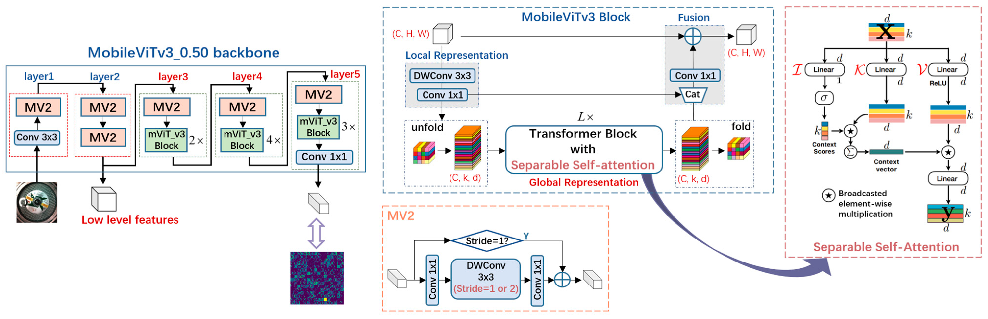
MobileViTv3 Backbone: Lightweight Convolutional Neural Networks (CNNs), such as XCeption and the MobileNet series [43,44,45], have been widely applied as the backbones of industry currently. With the continuous development of transformers in recent years, novel real-time backbones based on light-weight self-attention [46,47] and multi-head self-attention [48] have been introduced.
CNNs are limited by the local receptive fields. To acquire global information, CNNs require the additional attention mechanisms and the stacking of deeper networks, resulting in a larger number of parameters. By contrast, light-weight self-attention is more effective in capturing global long-range dependencies in the image patches, as it allows the patches to interact with each other through patch-wise cosine similarity calculation. Thus, it needs fewer parameters to achieve comparable, or even superior performance compared to traditional lightweight CNNs. Although its computational complexity is still higher than CNNs, its inference speed can meet the real-time needs. With the upgrading of hardware devices in the industry, the application prospects of lightweight transformers have greatly improved.
Among the light-weight ViTs, we have selected MobileViTv3_0.50 as the backbone for our proposed model for its highly efficient separable self-attention mechanism [47], which brings better feature extraction and generalizability while carrying fewer parameters than MobileNets.
The MobileViTv3 is of a hybrid architecture constructed by lightweight Inverted Residual block (MobileNetV2 block, MV2) and the MobileViTv3 block. The MobileViTv3 block is built upon its cornerstone—Separable Self-Attention.
The network structure (Figure 7) consists of five layers, with layers three to five incorporating the MobileViTv3 block, which stacks varying numbers of Separable Self-Attention modules in different layers. Additionally, a width factor is applied to adjust the scale of the feature channel dimension for each layer.
The following is the process of Separable Self-Attention. Assuming the input unfolded tensor is , firstly, it will be linearly projected using three branches, namely the Input, Key and Value, with three corresponding weights , and . Secondly, the results from the three branches will be used to calculate the representation of the input weighted by pixel-wise similarity. Finally, another linear projection with weights will be performed to produce the output. All in all, with the broadcasted element-wise multiplication operation denoted by , and softmax represented by , the process can be defined as:
Coordinate Attention: Coordinate Attention (CA) [19] is a light-weight attention mechanism which aggregates global semantic information along the H, W spatial directions on the input feature through 1D convolutional mappings. This approach can capture long-range dependency relationships along one spatial direction while preserving precise positional information along the other spatial direction, thereby distinguishing the localization of significant regions with a smaller computational complexity. The implementation of CA can be divided into two steps: coordinate information extraction and coordinate attention generation. The implementation details of CA are illustrated in Figure 8.
Coordinate Information Extraction is implemented by a pair of 1D Pooling layer along the H and W directions separately, with pooling kernel sizes of (H, 1) and (1, W). Assuming the input is , the output of channel c-th at height h or width w is calculated as:
Coordinate Attention Generation comprises a pair of 1D squeeze-and-excitation (SE) modules. Firstly, it concatenates the spatial-direction-aware features from the Coordinate Information Extraction, and then compresses the channel dimension of the features with a shared 1 × 1 convolution. Assuming the 1 × 1 convolution is denoted by , the channel compression rate is represented by r, and the activation function Hardswish(x) is regarded as , the output can be calculated by:
Secondly, the compressed features are split along the spatial directions into and , which will be processed by a pair of 1D convolutions ( and ), subsequently to restore the channel dimension. Lastly, a sigmoid activation is applied to generate attention weights along the H, W directions:
CA outputs a transformed tensor Y with augmented representations using the following Equation:
For the spatial patterns in the data, CA is the optimal mechanism for enhancing the overall network, as it efficiently captures spatial statistical information. Moreover, CA is highly lightweight, which aligns with the goals of this research.
3. DeeplabV3+ Based on Coordinate Attentioned-ASP (CA-ASP)
In general, to ensure reliable segmentation results, we have adopted the DeeplabV3+ segmentation framework, which provides more stable segmentation accuracy. The Encoder of DeeplabV3+ consists of a backbone and an ASPP module: the former is responsible for extracting basic features, while the latter highlights the multi-scale information interaction within the basic features, which adapt the network to the scale variations of different categories, thus providing robust segmentation results.
Aiming for enhancing segmentation accuracy through squeezing and integrating, rather than adding modules into the network, corresponding improvements are made to the DeepLabV3+ based on the characteristics of the datasets. Two main modifications are made to the original DeeplabV3+:
- Adopting the lightweight MobileViTv3_0.50 as the backbone.
- Replacing ASPP with the proposed lightweight CA-ASP module.
Figure 9 shows the structure of the improved DeeplabV3+ network.
For the backbone, in the pursuit of a extreme lightweight design, a width factor of 0.50 is chosen for the MobileViTv3. Furthermore, we extract features from layer two as low-level features and features from layer five as high-level features, which will serve as inputs of the decoder in two branches. Directly using the MobileViTv3_0.50 could avoid adding additional attention mechanisms to the CNNs backbones, which already contain larger parameters.
After embedding self-attention into the backbone, the next step we focus on is the ASPP module. How can we enhance the multi-scale contextual feature extraction capability of ASPP without increasing the computational load? Through analysis, we have discovered an interesting similarity between Coordinate Attention (CA) and ASPP, as well as how to make them a great pair in enhancing feature extraction capabilities, fused into the CA-ASP.
3.1. Analysis on the Computational Complexity of ASPP
ASPP (Figure 10) is the core module of the Deeplab series networks, which encode contextual information at multiple scales through convolution branches with different receptive fields.
The ASPP structure includes five branches:
- A 1 × 1 convolution for the smallest receptive field (single pixel) projection;
- Three atrous-separable-convolution branches extracting features with 3 different receptive fields, which produce multi-scale features;
- A pooling branch aimed at transforming the feature map into global statistical information and then regenerating them as features with the maximum receptive field, helping the network better understand overall semantics and improve its understanding of object context.
Ultimately, the concatenated multi-scale features are fused through a 1 × 1 convolution, which will impulse the interaction of the multi-scale information in the features.
In the Deeplab series, the output of the backbone, serving as the input of ASPP, usually contains a large channel dimension (such as 960, 1024, 2048, etc.) to preserve the integrity of feature information to the maximum extent. Figure 11 illustrates the segmentation accuracy of DeeplabV3+ with the MobileViTv3_0.50 with different output channel dimensions on the mean Intersection over Union (mIoU), highlighting the importance of high-dimensional output of the backbones.
Considering the case without bias, where is the input tensor and is the output tensor, using the kernel size of and the group of g, the Floating-Point Operations per second (FLOPs) of one convolution operation can be calculated as:
As can be seen in Figure 10, the five convolution branches in ASPP directly compute on the high-dimensional features with a larger , resulting in significant computational complexity.
3.2. Coordinate Attentioned-Atrous Spatial Pyramid (CA-ASP)
In our research, we have found that the global contextual feature extraction in CA mechanisms overlap in functionality with the ASPP pooling design. Based on this point, we first referred to the self-attention mechanism in pursuit of how global features interact with local features and how attention can be aggregated into the network, and then delicately integrate CA with ASPP. The proposed CA-ASP architecture is shown in Figure 12.
3.2.1. ASP: A Slimmed-Down ASPP without Pooling
At the first place, we simplified the ASPP to reduce its computational load. Modifications and corresponding analysis are as follows.
- 1 × 1 Conv as Pre-Mapping Unit.
First, on the assumption that a 1 × 1 convolution can be seen as a linear projection of the input features with an identity receptive field, rather than treating it as an independent branch in ASPP, we choose to move it forward as a pre-mapping unit to form an inverted residual block, which can reduce the dimensions of the input from into , without losing critical information. Different from directly mapping the features into a lower dimension, an inverted residual block enables the model to learn and retain critical information through a learnable “expand-and-squeeze” process (activations between the 1 × 1 convolutions are required). Figure 13 shows the details.
- Fusion to the features from four different receptive fields.
Figure 14 illustrates the comparison between random samples of the high dimensional input from the backbone and the output of the Pre-Mapping Unit , indicating a minor discrepancy between the two. This is because a single layer of linear projection by a 1 × 1 convolution would not introduce significant changes to the feature maps.
Thus, considering as the representation of , we import into the three branches of atrous-separable-convolution, with three different receptive fields to extract multi-scale contextual features. Then, concatenation is conducted on the above four contextual features from four different receptive fields. At last, the concatenated features will be fused by a 1 × 1 convolution layer to highlight the interaction of the multi-scale information.
- ASPP with no Pooling (Based on similarity between CA and ASPP).
There are multiple ways to obtain global features. ASPP Pooling employs a 2D Global Average Pooling (GAP) to spatially squeeze global statistical information with the maximum receptive field and then regenerate them into global features. Approximatively, CA can obtain a pair of global features along a certain spatial direction through 1D pooling, and then regenerate them into globally aware attention weights with 1D convolution.
From a functional perspective, there are overlaps between the two. Compared to the former, global features from the latter contains additional position information. Equation (7) illustrates that a pair of 1D pooling preserves positional information in two dimensions, while GAP can only preserve channel information. For semantic segmentation tasks, the latter would be the preferred option.
Based on this point, we decided to remove ASPP Pooling from ASPP, forming ASP. One question remaining is how to aggregate the global-aware weights from CA into the multi-scale contextual features from ASP.
3.2.2. Integrate CA into ASP
Now that the slimmed-down ASP has made room for CA, the second step is to integrate CA into the module.
One enlightenment brought by the Self-Attentions is that global information can be incorporated into the features, not only through concatenation [21,22,23,24,25,26] or addition [14,20], but also through weighted multiplication [6,7,46,47,48]. Separable Self-Attention is a classic structure of Self-Attentions, and CA is a typical case of attention mechanisms. By comparing Equations (1) and (5), we can find that CA multiplies the weights with the input features, while Separable Self-Attention multiplies the weights with the representation of the input. Both ways can incorporate global attention information into the features. This evidence proves that CA could replace ASPP Pooling.
Inspired by this, we use from the Pre-Mapping as input of CA to generate globally aware coordinate attention weights and then multiply it with the multi-scale contextual representation of the input produced by the ASP.
3.2.3. Mathematical Description and Effects
Assuming that the output from the backbone is , the Pre-Mapping Unit is denoted by , the atrous-separable-convolutions with a atrous rate i is represented by , and fusion is signified by , operations of the ASP can be described as:
Secondly, we can take as the input to calculate CA weights according to Equations (2)–(4). Modifying Equation (5) with Equation (8) yields the output of CA-ASP as:
Table 2 lists the ASPP combined with different attention mechanisms. It is evident that CA-ASP significantly reduces the parameter size (45.3%) and the computational load (53.2%) of ASPP. Further experimental results indicate that this change does not have a negative impact on the model’s performance, which will be detailed in Chapter 5.
3.3. Loss Function: Weighted Cross-Entropy
To address the issue of class imbalance, we use Weighted Cross-Entropy (WCE) as the loss function. Assuming that C is the category number, stands for the weight of class c, is the label value of the i-th pixel, and is the predicted value. The WCE can be calculated using Equation:
The weights are calculated based on the total pixels of each class, where represents the total pixels for the i-th class in the annotated data, f denotes the total pixels, and eps is a very small number to prevent division by zero. The weight for the i-th class is calculated by:
By taking the logarithm, classes with lower frequencies receive higher weights, thereby increasing their contribution to the loss function. WCE has the advantage of simple gradient computation and easy convergence properties. By manually calculating class weights, it spares the model from learning different penalty levels for different classes during training, thereby reducing the training burden. In cases where the dataset is relatively complete, it is a suitable and efficient option.
4. Training Strategies: Self-Supervised Pre-Training and Transfer Learning
In seeking further boosting in segmentation performance without an additional calculation workload, our focuses have shifted to training strategies.
4.1. Self-Supervised Pre-Training Based on the Hybrid MAE
In our viewpoint, self-supervised pre-training enhances the model’s capacity for capturing crucial information by reinforcing its understanding of semantic information in the data, which includes the distinguishing information of the minority classes. Therefore, self-supervised pre-training has the potential to ease class imbalance by augmenting the overall semantic extraction capabilities on all categories.
On the other hand, self-supervised pre-training is highly suitable for defect segmentation in the industry, as there exists inexhaustible data that are free to be used.
Nevertheless, existing networks have strong architectural constraints, with MAE and semMAE based on a full transformer architecture, and FCMAE built upon fully convolutional layers, making it difficult to be applied directly on the hybrid architectural MobileViTs [46,47,48]. Thus, we have developed a Hybrid MAE network.
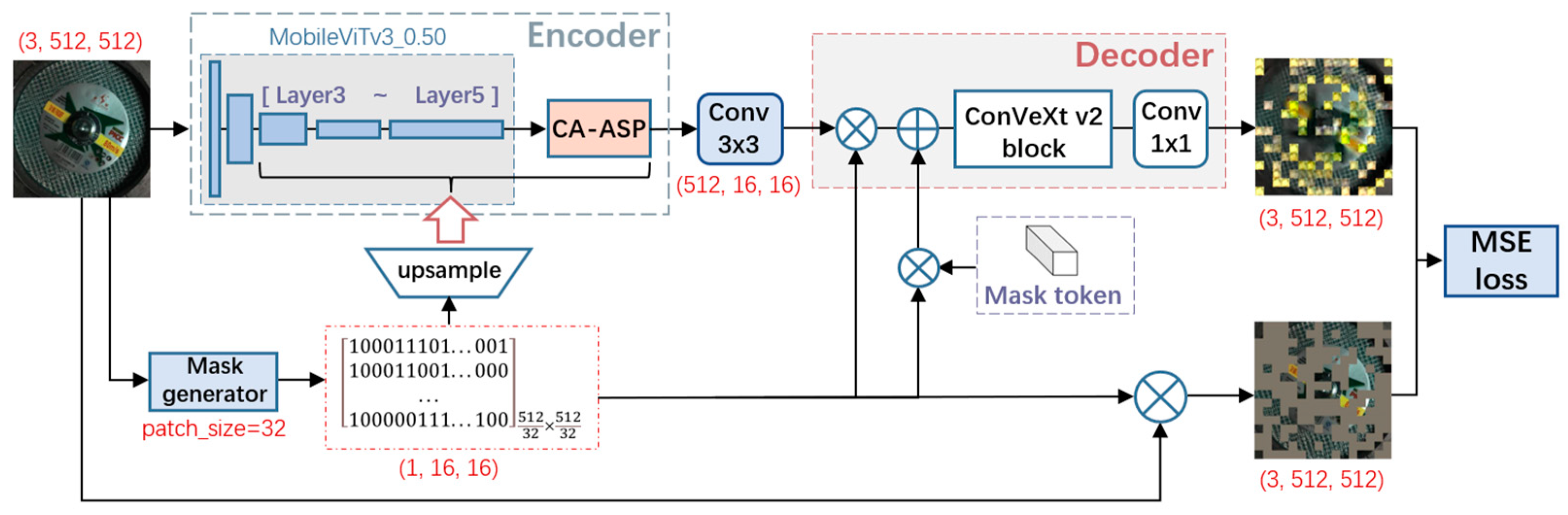
The key idea of MAE is to divide input images into patches of a certain patch size, which will be randomly masked with a relatively high mask rate (0.60, 0.75, etc.), and then to reconstruct the missing pixels through the pretraining model of encoder–decoder architecture, forcing the model to conduct self-supervised learning on the data (Figure 15). After pretraining, the semantic-aware encoder will be transferred into the networks in the downstream task.
All the related methods [39,40,41] adopt an asymmetric encoder–decoder structure, where a relatively larger encoder is paired with a light-weight decoder, allowing the encoder to take on more of the semantic feature extraction burden. Additionally, the encoder only extracts features from the remaining visible patches, significantly reducing the model’s computational complexity and accelerating the pretraining process.
To apply self-supervised pre-training on the MobileViTv3 of hybrid architecture with both CNN and Transformer blocks, modifications are made based on the MAE and FCMAE. The overall structure of the proposed pre-training network is shown in Figure 16.
4.1.1. Mask Generation
Assuming the input image is , the patch size is set to 32, and the mask rate is chosen as 60%, a mask matrix is generated at the patch-wise level.
4.1.2. Encoder
We take the whole structure of the encoder in DeeplabV3+ for pretraining, which includes a MobileVITv3_0.50 backbone and the CA-ASP. To conduct masking, some details need to be noted.
- Layers for masking:
Convolutional layers, limited by the receptive field, especially for those in the initial stages, may not be capable of learning sufficient semantic information from the sparsely masked data, which could be detrimental to the training of subsequent layers. Therefore, to prevent excessive information loss caused by early masking, we have drawn inspiration from FCMAE to mask features on the later stage, with layer three to layer five of the MobileViTv3, as well as the CA-ASP layer selected for masking. Owing to the varying size of the features in different layers, the mask matrix needs to be upsampled before application.
- Masking strategies:
To ensure that the encoder extracts features only from visible pixels after masking, for convolutional layers in the backbone, we apply the approach purposed in FCMAE [41] (Figure 17a), conducting a binary masking operation before and after every convolution operation. Since a lightweight encoder is selected for the task, this operation will not bring too much computational burden. However, when we tried to implement the same method to CA-ASP, one problem arises: how do we match the 2D mask matrix with the 1D convolution in CA? To avoid mismatching and streamline the masking process, we treat CA-ASP as a black box and only apply masking to its input and output (Figure 17b). During fine-tuning, all it needs is to simply remove the masking steps.
Additionally, for the separable self-attention layer, the method of MAE [39] is applied (Figure 17c), where self-attention is only conducted on the unfolded non-masked parts. Then, the transformed features will be reassembled in the original order. Since self-attention occupies most computations in the encoder, it would accelerate the pretraining.
4.1.3. Decoder
The decoder is designed, based on FCMAE, with a few adjustments tailored for the DeeplabV3+. In semantic segmentation, it is essential to maintain an adequate feature size from the encoder, hence an output stride of 16 is commonly selected for such tasks, which the produces the output features . This process can be described as:
- Adjustment for the output stride of the encoder in semantic segmentation:
However, in the FCMAE method, there is no upsampling process. To match the shape of predict tensor and the input image, the final prediction needs to be scattered across the channel dimension in a patch-wise order.
Assuming the patch size is set to 32, the corresponding number of patches will be 162. The final prediction needs to be , where the first dimension represents all the pixels in each patch and the second dimension represents the number of patches.
To ensure consistency with the encoder throughout pre-training and fine-tuning, the feature maps need to be downscaled by half, which will be achieved via a 3 × 3 convolution with a stride of 2. Moreover, to preserve the integrity of the information extracted from the encoder, the channel dimension of the features should be expanded simultaneously. With representing the output from the encoder, the output of this downscale mapping layer would be:
- ConvNeXtV2 block in FCMAE:
The following ConvNeXtV2 block [41] in FCMAE is an inverted residual structure (Figure 18). To manage sparse data, it uses a large convolutional kernel and a corresponding stride to increase the receptive field while remaining in the shape of the input, allowing it to aggregate information from the sparse visible pixels to the maximum extent. Within ConvNeXtV2, there exists a Global Response Normalization (GRN) module [41] to address the issue of feature collapse, which refers to the phenomenon where features become excessively similar.
The following elucidates the implementation of the GRN. Given that an input , a L2-Norm is applied, followed by a normalization function . To ease optimization, two additional learnable parameters, denoted by and , were introduced and initialized to zero. The output can be calibrated as:
The output of the ConvNeXtV2 Block would be:
- Prediction Layer:
At last, the prediction layer is conducted by a simple 1 × 1 convolution, which transforms the features into a final prediction:
4.1.4. Loss Function
The Mean Squared Error (MSE) is used as the loss function, calculating the average loss of each patch only on non-masked pixels.
Firstly, the input X and prediction Y should be transformed into a patch-wise level:
Assuming that p is standing for the total number of patches, the mask value of the i-th patch is denoted by , l is the total pixels in the i-th patch, is the j-th pixel in the i-th patch of the prediction, with corresponding ground truth signified by , the loss can be calibrated as:
4.2. Transfer Learning for the Reverse Task
The obverse task is selected as the upstream task, due to its richer semantic information. After self-supervised pre-training with MAE and the subsequent supervised fine turning on the obverse set, the model is already excellent in extracting semantic information. Thereby, we opted not to conduct additional MAE pre-training for the reverse task, but directly transfer the model weights from the obverse task to the reverse one.
Unlike MAE pretraining, which only delivers the encoder of the network, transfer learning between the dual tasks involves transferring the entire network structure, except for the final prediction layer, owing to the distinct number of categories presented in the two sets.
This strategy leverages the knowledge and feature representations learned from the upstream task to expedite the training process of the reverse task, potentially enhancing model performance.
5. Results
5.1. Experimental Setup
All the designed experiments were conducted on the Window 11 system with the 13th Gen Intel(R) Core (TM) i9-13900HX CPU, 16.0 GB RAM, and NVIDIA GeForce RTX 4060 GPU with 8 GB memory. The implementation of the developed models and methods are based on the PyTorch 2.1.1 framework with CUDA 11.2, CUDNN 11.2.
5.1.1. Dataset and Loss Function
Experiments were conducted using image data with a resolution of .
For supervised learning, the annotated datasets were split into training, validation, and testing sets in a 6:3:1 ratio. Subsequently, standard data augmentation techniques (random flipping, rotation, scaling, cropping, etc.) were applied, resulting in a threefold increase in the data volume of each set.
The training and validation sets were used for supervised training, parameters optimization, and result evaluation, while the testing set was used for the final segmentation demonstration.
All the networks in the experiment were trained using Weighted Cross-Entropy.
For MAE self-supervised pre-training, we have made full use of the 1295 unannotated original samples on the obverse task.
5.1.2. Evaluation Indicators
- Metrics of overall segmentation accuracy: Two metrics were used to verify the overall segmentation accuracy.
- Mean Pixel Accuracy (MPA): MPA calculates the average pixel-level segmentation accuracy, but it does not consider the spatial relationships between categories, and it is insensitive to segmentation boundaries;
- Mean Intersection over Union (mIoU): mIoU measures the average overlap between predicted masks and ground truth masks across all classes in a dataset. It is the most widely accepted and primary metric among all the other metrics to evaluate the overall segmentation accuracy as it considers not only pixel-level accuracy but also the accuracy of segmentation boundaries;
- Metrics for class imbalance: Due to the significant class imbalance, we adopt two auxiliary metrics to assess the model’s ability to address this issue.
- Intersection over the Union (IoU) of the minority classes: IoU measures the overlap between predicted masks and ground truth masks for a certain class. We will provide extra attention to the IoU of the minority classes in the results;
- Frequency Weighted Intersection over the Union (FWIoU): FWIoU computes a weighted sum of IoU for each category, with the weights being the frequency of occurrence of each category.
In Equations (20)–(23), n represents the number of target categories, indicates represents the total pixels correctly predicted as an actual category, and denote the total pixel-wise mispredictions of a certain category.
- Metrics for measuring lightweighting and computational complexity: The three metrics below are calculated on the obverse set, as it contains more categories which result in larger number of parameters compared to the reverse set. Metrics in this part will determine whether the network meets the real-time requirements of Grinding Wheel defect segmentation.
- Parameter Size (in Million, M): Parameter size refers to the total number of learnable parameters in a model, measured in millions (M), which intuitively reflect the scale of the network. Additionally, it is important to note that parameter size is not equivalent to memory usage (in MB). Typically, each parameter is stored using a precision floating-point format (float32). Hence, the memory usage of a network can be estimated by multiplying the parameter size by 4;
- Floating-point Operations (FLOPs) (in Million times, M): FLOPs are the most commonly used and intuitive metric for measuring model computational complexity;
- Latency (in ms): Latency is measured as the average speed of 50 consecutive inferences of an input with a shape of , verifying the inference speed.
5.2. Experiments on the Obverse Task
5.2.1. Ablation Experiments of the CA-ASP
To evaluate the effectiveness of CA-ASP, we compared the combination of ASPP with various state-of-the-art attention mechanisms. The experiments were conducted with the DeeplabV3+ network based on the MobileViTv3_0.50 backbone, each trained for 250 epochs with a batch size of 10. The metrics on the validation set of each model are listed in Table 3.
As can be observed from the results, our CA-ASP method, which has a reduced parameter size (−0.87 M) and FLOPs (−649.29 M) compared to the baseline model, gains the highest mIoU score of 70.208%, surpassing other methods by +0.849% to +2.996%.
However, compared to one of the best combinations “ASPP + CA”, our method has shown a slight inadequate performance on the challenging class Logo.
To further explore the potential of CA-ASP, we have proceeded to conduct MAE self-supervised pretraining on the model.
5.2.2. Ablation Experiments of MAE Self-Supervised Pretraining
In this part, we used the DeeplabV3+ based on MobileViTv3_0.50 backbone and CA-ASP on the obverse task, where 1295 unannotated data were divided into training and validation sets in an 8:2 ratio. Pretraining was conducted for 800 epochs with a batch size of 20. In the formal training phase, models using MAE pretrained weights and initial weights were separately trained for 250 epochs.
- Changes in the metrics.
To measure the differences in segmentation performance brined by the MAE method, we first looked at the changes in the metrics (Table 3), which indicate that the network with MAE achieved a slight increase in mIoU (+0.588%) and FWIoU (+0.043%) but obtained a relatively significant improvement in the IoU of the challenging classes, especially in Ring_NG, exceeding the CA-ASP model by +4.652% and the baseline ASPP model by +5.604%, while in the category Logo, surpassing the best combination of “ASPP + CA” by +0.729% and baseline model by +7.297%.
- mIoU-over-epoch curves.
Additionally, a reference was made to the mIoU-over-epoch curves in Figure 19, which indicates that MAE has brought a better initial state to the model, but soon began to converge with the baseline, eventually resulting in a minimal rise.
This has prompted us into rethinking about how to evaluate the quality of semantic information learning during self-supervised pretraining. In situations where there is an imbalance between categories, the tendency of the model towards some certain categories may lead to a lack of improvement in mIoU. Also, a light-weight network has fewer parameters to be trained, which may result in similar converging speed after the initial phase. Furthermore, the absence of pre-training for the decoder, as well as the disparity between the source domain (Image Reconstruction) and the target domain (Semantic Segmentation) may contribute to the similar convergence in the later stage.
- IoU-over-epoch curves.
Based on this assumption, we observed the changes in IoU of each class (Figure 20) and found that in the initial stage, the model’s understanding on the Background far exceeds that of the baseline. At the same time, there has been some improvement in the majority classes, Mesh and Sand. In contrast, the model did not demonstrate any additional benefits from pre-training considering no difference was made in the two difficult classes Ring_NG and Logo during the initial training.
In fact, this situation accords with expectation, as during pretraining, there is no concept of categories, meaning that the majority pixels, which belong to the majority classes over supervised training, contributing more to the MSE loss, inevitably leading to a certain overfitting. The higher stability of the two majority classes, Mesh and Sand, in subsequent training also serves as evidence of this point.
However, to our surprise, in the following training for the challenging class Ring_NG, while the baseline model had already started to converge, the IoU of the MAE model was still rising, ultimately leading to a significant improvement in segmentation accuracy. Meanwhile, although both curves of the Logo class exhibited significant fluctuations, which stem from its extreme scarcity, the MAE method still achieved a higher metric value. Furthermore, when we observed the period during which the two challenging classes reached their optimum, there was a minor difference shown in the IoU of the two models on other categories as they were already converging. This means that the increase in mIoU is mostly contributed to by challenging classes, which would provide valuable guidance for addressing imbalance phenomenon.
The reason behind this may lie in the additional samples, which latently exist in the unannotated data and the semantic-aware pretrained weight which contains a more comprehensive understanding of the minority classes. One the one hand, the additional samples are beneficial for the model to learn more semantic information. On the other hand, during the initial stages of training, due to the issue of imbalance, the majority classes still contribute the most to the loss, prompting the model to fit towards the majority. At this point, the benefit of a difficult-class-friendly initial weight may not have fully manifested. However, when other majority classes start to converge with a relatively high mIoU, their contribution to loss decreases significantly, and the minority classes come to dominate. It is at this stage that a semantic-aware initialization weight, compared to random initialization, has greater potential to steer the model’s convergence towards the challenging classes.
- Improved Quality of Features from the Encoder.
Figure 21 demonstrates the feature from the encoder of DeeplabV3+ before and after supervised training, where (a) employs randomly initialized weights, and (b) utilizes pre-trained weights with MAE. The input is the image from the second row of Figure 22 in Section 5.2.3, which contains a Ring_OK and a Ring_NG object.
A notable enhancement in the quality of features is observed with the MAE method. Furthermore, upon closer inspection of the features, it is evident that there are more distinct features highlighting Ring_OK. Additionally, the features of Ring_NG are more pronounced compared to the randomly initialized approach.
In conclusion, this further validates our hypothesis of using MAE to address class imbalance. MAE pre-training significantly enhances the network’s understanding of the minority classes. Additionally, it is noticeable that the model with MAE has significantly reduced the cluttered and irrelevant features. This is because the model filters out the background features and retains only the most important features for the current sample, which indicates that the model’s ability to focus on important information has also been further improved.
5.2.3. Comparative Experiments with State-of-the-Art Methods
At last, we have reached the comparative experiment to determine if the proposed model is sufficiently ideal compared to some state-of-the-art real-time models. We have involved four different segmentation architecture including FCN [49], PSPNet [50], and Segformer [51] and DeeplabV3+. Moreover, two types of backbone have been selected, including the MobileNetV3, renowned as one of the best real-time CNNs, and the MobileViTv3, which is one of the top-performing real-time hybrid transformers.
The first experiment is the metrics comparison (Table 4), according to which we make the following observations:
- DeeplabV3+ is slower than other simple architecture, but better in segmentation precision: FCN, PSPNet, and Segformer are typical asymmetric encoder–decoder structures, where the decoder is considerably simpler than the encoder. Hence, when given a light-weight encoder, it would exhibit faster inference speeds. However, when we compare Methods (1)–(3) and (6), it becomes evident that models of such structure all suffer from one issue: they attain an excellent MPA but struggle to achieve a sufficient mIoU, which means that the model is capable of accurately predicting most areas (profit for MPA) but fails to produce precise mask boundaries (adverse to mIoU).
- In the perspective of latency, our method bridges the gap between CNNs and hybrid transformers: Experimental results in other research [46,47,48] have shown that lightweight CNNs are still faster than lightweight hybrid transformers. When we refer to Methods (4)–(8), it is evident that the models based on MobileViTv3 contain fewer parameters but obtain lager FLOPs, which stem from the mechanism of self-attention, optimizing the limited parameters to perform denser computations to achieve superior segmentation precision.Among the DeeplabV3+ models, our method contains the fewest parameters, which is 45.2% smaller than models with the MobileNetV3_large, and 41.4% smaller than the one using the MobileViTv3_0.75. The FLOPs of our method is between the above two models and is closely comparable to the one using the MobileNetV3_large (+1,789.88 M), which on the GPU device will provide minimal differences in the latency (+0.146 ms).All in all, the latency of 9.512 ms in our method can meet the real-time requirement. Moreover, this result can provide valuable insights for improving real-time transformer-based semantic segmentation models: if the computational complexity of self-attention cannot be further reduced, then improvements can be made to the ASPP module to achieve faster inference speeds.
- Among the Deeplabs, our method obtains the best mIoU, with the smallest parameter size: It is apparent that our method, with the best mIoU of 70.796%, surpasses other Deeplabs ranging from +2.463% to +0.597%. Furthermore, this improvement is achieved with the parameters reduced to a minimum.
- Ability for dealing with imbalance: It can be observed from the FWIoU and IoU that our method presents notable advantages in addressing imbalance. In terms of FWIoU, our method gains the highest score of 89.133%. For the IoU of the challenging classes, other methods encounter difficulty in balancing the segmentation precision across both classes. However, this phenomenon is effectively addressed by our method as there is a significant improvement in the IoU of the two classes.
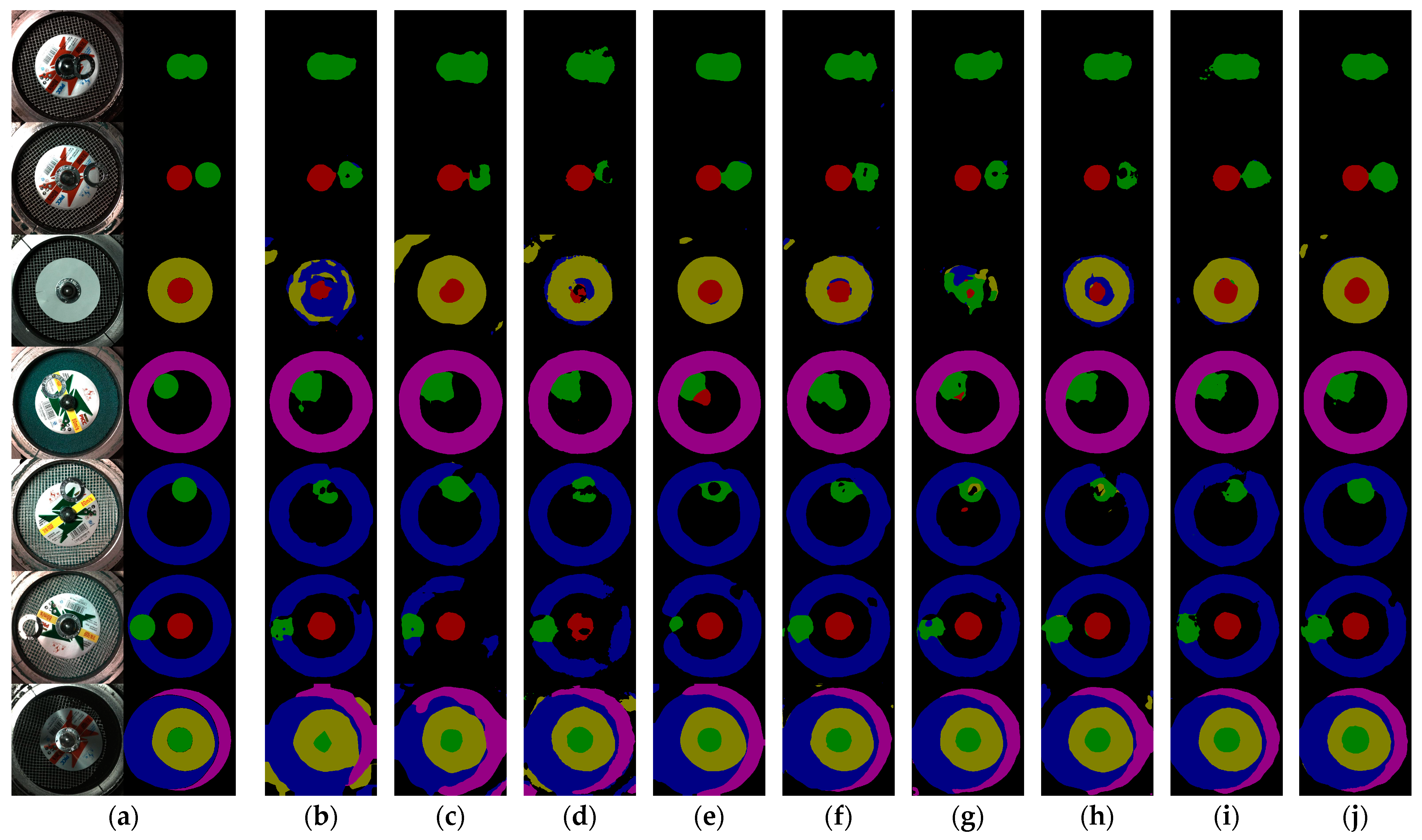
The second experiment aims to evaluate the model’s stability and generalizability on unseen data in the testing set. Figure 22 demonstrates some of the visualized segmentation results on the testing set. As we move along from Row 1 to Row 7, the complexity of the segmentation scene gradually increases, which poses high demands on the model’s generalizability and stability. Moreover, we have further involved the DeeplabV3+ with the “ASPP + CA” method into the demonstration, as it has produced excellent results, according to Table 3.
In Table 3 and Table 4, it is proven that our method achieves the highest segmentation precision on both mIoU and FWIoU. In Figure 22, it is more intuitive to make observations that may help to discern the underlying reason:
- Smoother boundaries brought by lager parameters: PSPNet and the DeeplabV3+ with the MobileNetV3_large are constructed by the largest parameters compared to other models, and thus they have provided smoother mask boundaries.However, smoothness is not equivalent to precision. In the relatively simpler scenes (Row 1~3), Methods (c), along with (b) and (d), present insufficient segmentation accuracy. As the scenes become increasingly complex, Methods (c) and (e) exhibit more pronounced misclassifications (Method (c) in Row 5~6, Method (e) in Row 4~6), some of which is caused by its shortcomings in segmenting the challenging Ring_NG and correctly predicting the category of a moderately sized region.
- The stability of segmentation accuracy unaffected by scene complexity: Segmentation in complex scenes not only tests the overall segmentation accuracy of the model but also requires the model to sensitively discern precise boundaries. Additionally, it poses high demands on how the model balances different categories. When multiple segmentation categories coexist, the model may expand the regions of majority classes (including the Background) and engulf those of minority classes. This reflects the model’s ability in addressing class imbalance. Methods (b)-(e) and (g)-(h) show discrepancies as the scene becomes more complex, especially in the challenging classes of Ring_NG and Logo.When we observe Row 7, another phenomenon emerges: as the scene becomes sufficiently complex, some methods, including (c), (e) and (h), tend to expand the segmented regions outwards. This could be a contributing factor to the lack of improvement in the mIoU metric: the denominator, represented by the Union, becomes larger.Overall, compared to the best-performing methods (e), (f), and (h), our approach demonstrates the fewest misclassifications and ensures the most precise boundaries of Ring_NG and Logo, and thus maintains solid stability and better generalizability as the scene complexity increases, thanks to the enhanced attention capability of CA-ASP on spatially salient regions, which significantly improves the accuracy of the baseline (g) with fewer parameters, and the improvement in addressing imbalance through MAE self-supervised pretraining.
5.3. Experiments on the Reverse Task
5.3.1. Ablation Experiments of Transfer Learning
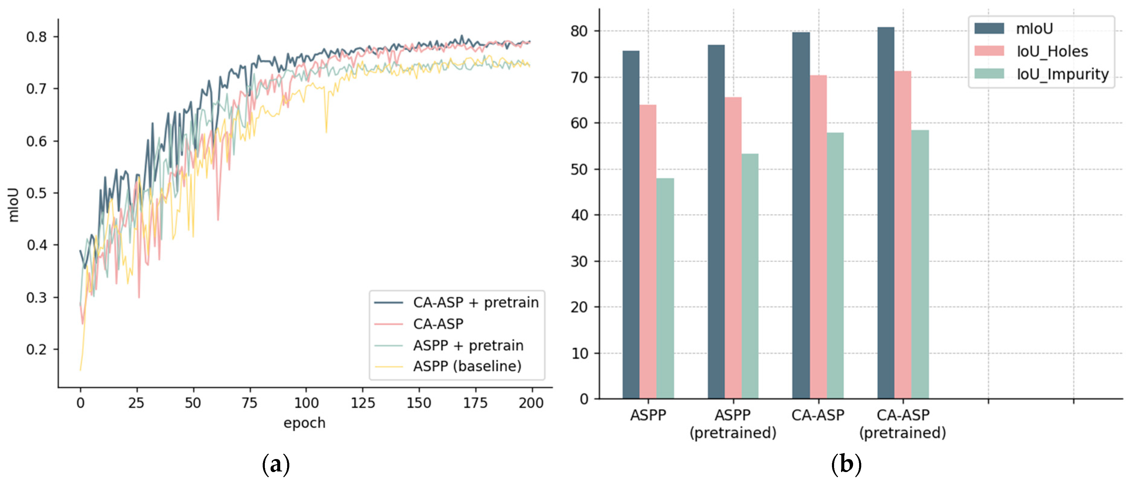
To verify the effectiveness of transfer learning on the reverse set, we compared the mIoU-over-epoch curves of two sets of models with and without pretrained weights (Figure 23), one being the baseline model using the DeeplabV3+ with mobileViTv3_0.50 backbone, and the other being our proposed model with CA-ASP.
At the initial and middle stages, benefitting from the complete pretraining weights of both the encoder and the decoder, a faster convergence was achieved through transfer learning. As the models began to converge, models with transfer learning pretrained weights obtained a slight rise in the mIoU.
The results indicate that transfer learning not only accelerates convergence but also, by further training on the semantic-aware pretraining weights, leads to a higher segmentation accuracy.
5.3.2. Comparative Experiments with State-of-the-Art Methods
We have further validated the effectiveness of our network in the reverse task by comparing several models that performed well in the obverse task. Each network is trained for 200 epochs with a batch size of 10.
- Achieving the best performance on overall precision and dealing with imbalance.
Firstly, in Table 5, results indicate that, consistent with the obverse task, our method achieves the best segmentation performance on mIoU (80.757%), which has brought a +5.216% increase compared to the baseline.
In terms of imbalance, simple networks such as PSP and Segformer, show limitations in handling challenging classes in the reverse set. In contrast, our method achieves significant improvement in the Holes (+4.233%~+11.816%) and Impurity (+5.17%~+21.738%) compared to other methods.
- Magnified gaps between different methods caused by the more complex scenes.
Secondly, in addition to the metrics itself, another noteworthy phenomenon is that on the reverse task, the gaps between the models have been magnified. To further explore the reasoning behind this, likewise, we have assessed the models on the testing set, which will also test the stability and generalizability of the models on the reverse task.
As in Figure 22, the complexity of the scene in Figure 24 increases progressively in order, which vividly illustrates the accuracy discrepancies between the models.
As stated in Section 2.2.3, the scenes are more complex in the reverse set. The phenomenon of expanding segmented regions outwards in complex scenes, as depicted in Figure 22, becomes intensified in the reverse set excessively. Even in the simplest scenario in Row 1, Method (d) exhibits such a situation. As the scenes become more complicated (Row 4~7), the excessive expansion, to varying degrees, is shown in most of the methods (b)-(g), which will hinder the networks to achieve higher mIoU scores.
However, under such circumstances, our method (h) still processes robust stability and better generalizability across different scenes, as it effectively suppresses the excessive expansion of the regions, which leads to sharper boundaries. On the other hand, it can be perceived in the masks of Holes and Impurity that, our method produces the clearest and most precise edges on the challenging classes even in the most complicated scenarios.
6. Conclusions and Discussion
Targeting at extreme lightweight and highly efficient design for the DeeplabV3+, this paper has proposed a novel light-weight CA-ASP module to the DeeplabV3+ network based on the discovery of similarities between CA and ASPP, which outperforms the original ASPP baseline with a reduced parameter size (45.3%) and computational complexity (53.2%). Moreover, in addition to employing Weighted Cross-Entropy, this paper has innovatively developed a hybrid MAE self-supervised pre-training network to manage imbalance. Through the MAE pretraining, we have fully leveraged the unannotated data to uplift segmentation precision of the minority categories, and further enhance the overall precision. At last, to address the highly related dual-side tasks, transfer learning has been conducted to accelerate the convergence process, which has further led to an improvement in segmentation accuracy on the reverse set.
Ablation experiments results have indicated that our network, with a real-time inference speed of 9.512 ms, achieves fewer parameters (−0.87 M) and less FLOPs (−649.29 M) compared to the baseline network using ASPP, while surpassing the latter on mIoU by +2.463% on the obverse set and +5.216% on the reverse one. Comparative results have demonstrated that our method exceeds other state-of-the-art real-time semantic segmentation networks on mIoU by +0.597%~+4.124% on the obverse set and by +3.638%~+8.742% on the obverse set. Moreover, our network has made significant improvements in managing imbalance and has shown robust stability and a better generalizability in complex scenarios.
Through dual validations on the obverse and reverse sets, results have demonstrated that our developed method provides valuable answers to the two main questions proposed by the dual grinding wheels segmentation tasks.
However, after careful review, two issues were identified. Firstly, no modification has been made to the decoder of the DeeplabV3+, which has a great potential for further enhancing segmentation performance. Secondly, we have made structural improvement to MAE on the hybrid architecture encoder but did not change the form of self-supervised pre-training. Given the potential of MAE in addressing imbalance issues, there may be better strategies, such as selectively choosing difficult samples of the minority classes to fine-tune the pre-training. On the bright side, as in general, the attention mechanisms contain a pooling layer, there may be more ways to integrate different attention mechanisms into the ASPP according to the theory we proposed. These topics require further exploration in future research.
Author Contributions
Conceptualization, Y.L. and P.Z.; Methodology, Y.L. and C.L.; Software, Y.L. and C.L.; Validation, Y.L. and C.L.; Formal analysis, P.Z.; Investigation, Y.L. and P.Z.; Resources, P.Z. and H.W.; Data curation, Y.L. and C.L.; Project administration, P.Z. and H.W.; Supervision, Y.L., P.Z. and H.W.; Visualization, Y.L. and C.L.; Writing (original draft), Y.L. and C.L.; Writing (review and editing), P.Z. and H.W.; Funding acquisition, H.W. All authors have read and agreed to the published version of the manuscript.
Funding
This research was funded by the National Natural Science Foundation of China (No. 62171142); Natural Science Foundation of Guangdong Province (No. 2021A1515011908); Jihua Laboratory Foundation of the Guangdong Province Laboratory of China (No. X190071UZ190).
Data Availability Statement
Data in this study are partly available on reasonable request from the corresponding authors.
Conflicts of Interest
The authors declare no conflicts of interest.
References
- Tulbure, A.; Tulbure, A.; Dulf, E. A review on modern defect detection models using DCNNs–Deep convolutional neural networks. J. Adv. Res. 2022, 35, 33–48. [Google Scholar] [CrossRef] [PubMed]
- Bhatt, P.M.; Malhan, R.K.; Rajendran, P.; Shah, B.C.; Thakar, S.; Yoon, Y.J.; Gupta, S.K. Image-Based Surface Defect Detection Using Deep Learning: A Review. J. Comput. Inf. Sci. Eng. Comput. Inf. Sci. Eng. 2021, 21, 040801. [Google Scholar] [CrossRef]
- Yang, J.; Li, S.; Wang, Z.; Dong, H.; Wang, J.; Tang, S. Using deep learning to detect defects in manufacturing: A comprehensive survey and current challenges. Materials 2020, 13, 5755. [Google Scholar] [CrossRef] [PubMed]
- Usamentiaga, R.; Lema, D.G.; Pedrayes, O.D.; Garcia, D.F. Automated surface defect detection in metals: A comparative review of object detection and semantic segmentation using deep learning. IEEE Trans. Ind. Appl. 2022, 58, 4203–4213. [Google Scholar] [CrossRef]
- Zhang, H.; Liu, H.; Kim, C. Semantic and Instance Segmentation in Coastal Urban Spatial Perception: A Multi-Task Learning Framework with an Attention Mechanism. Sustainability 2024, 16, 833. [Google Scholar] [CrossRef]
- Guo, M.H.; Lu, C.Z.; Hou, Q.; Liu, Z.; Cheng, M.M.; Hu, S.M. SegNeXt: Rethinking Convolutional Attention Design for Semantic Segmentation. Adv. Neural Inf. Process. Syst. 2022, 35, 1140–1156. [Google Scholar]
- Dosovitskiy, A.; Beyer, L.; Kolesnikov, A.; Weissenborn, D.; Zhai, X.; Unterthiner, T.; Dehghani, M.; Minderer, M.; Heigold, G.; Gelly, S. An image is worth 16x16 words: Transformers for image recognition at scale. arXiv 2020, arXiv:2010.11929. [Google Scholar]
- Cumbajin, E.; Rodrigues, N.; Costa, P.; Miragaia, R.; Frazão, L.; Costa, N.; Fernández-Caballero, A.; Carneiro, J.; Buruberri, L.H.; Pereira, A. A Systematic Review on Deep Learning with CNNs Applied to Surface Defect Detection. J. Imaging 2023, 9, 193. [Google Scholar] [CrossRef]
- Chen, L.; Papandreou, G.; Kokkinos, I.; Murphy, K.; Yuille, A.L. Semantic image segmentation with deep convolutional nets and fully connected crfs. arXiv 2014, arXiv:1412.7062. [Google Scholar]
- Chen, L.; Papandreou, G.; Kokkinos, I.; Murphy, K.; Yuille, A.L. Deeplab: Semantic image segmentation with deep convolutional nets, atrous convolution, and fully connected crfs. IEEE Trans. Pattern Anal. Mach. Intell. 2017, 40, 834–848. [Google Scholar] [CrossRef]
- Chen, L.; Papandreou, G.; Schroff, F.; Adam, H. Rethinking atrous convolution for semantic image segmentation. arXiv 2017, arXiv:1706.05587. [Google Scholar]
- Chen, L.; Zhu, Y.; Papandreou, G.; Schroff, F.; Adam, H. Encoder-decoder with atrous separable convolution for semantic image segmentation. In Proceedings of the European Conference on Computer Vision (ECCV), Munich, Germany, 8–14 September 2018; pp. 801–818. [Google Scholar]
- Hu, J.; Shen, L.; Sun, G. Squeeze-and-excitation networks. In Proceedings of the IEEE Conference on Computer Vision and Pattern Recognition, Salt Lake City, UT, USA, 18–23 June 2018; pp. 7132–7141. [Google Scholar]
- Fu, J.; Liu, J.; Tian, H.; Li, Y.; Bao, Y.; Fang, Z.; Lu, H. Dual attention network for scene segmentation. In Proceedings of the IEEE/CVF Conference on Computer Vision and Pattern Recognition, Long Beach, CA, USA, 16–17 June 2019; pp. 3146–3154. [Google Scholar]
- Pan, Y.; Zhang, L. Dual attention deep learning network for automatic steel surface defect segmentation. Comput. Civ. Infrastruct. Eng. 2022, 37, 1468–1487. [Google Scholar] [CrossRef]
- Chollet, F. Xception: Deep learning with depthwise separable convolutions. In Proceedings of the IEEE Conference on Computer Vision and Pattern Recognition, Honolulu, HI, USA, 21–26 July 2017; pp. 1251–1258. [Google Scholar]
- Liu, Q.; El-Khamy, M. Panoptic-Deeplab-DVA: Improving Panoptic Deeplab with Dual Value Attention and Instance Boundary Aware Regression. In Proceedings of the 2022 IEEE International Conference on Image Processing (ICIP), Bordeaux, France, 16–19 October 2022; IEEE: Piscataway, NJ, USA, 2022; pp. 3888–3892. [Google Scholar]
- Woo, S.; Park, J.; Lee, J.; Kweon, I.S. Cbam: Convolutional block attention module. In Proceedings of the European Conference on Computer Vision (ECCV), Munich, Germany, 8–14 September 2018; pp. 3–19. [Google Scholar]
- Hou, Q.; Zhou, D.; Feng, J. Coordinate attention for efficient mobile network design. In Proceedings of the IEEE/CVF Conference on Computer Vision and Pattern Recognition, Nashville, TN, USA, 20–25 June 2021; pp. 13713–13722. [Google Scholar]
- Liu, R.; Tao, F.; Liu, X.; Na, J.; Leng, H.; Wu, J.; Zhou, T. RAANet: A Residual ASPP with Attention Framework for Semantic Segmentation of High-Resolution Remote Sensing Images. Remote Sens. 2022, 14, 3109. [Google Scholar] [CrossRef]
- Li, Y.; Cheng, Z.; Wang, C.; Zhao, J.; Huang, L. RCCT-ASPPNet: Dual-Encoder Remote Image Segmentation Based on Transformer and ASPP. Remote Sens. 2023, 15, 379. [Google Scholar] [CrossRef]
- Zhang, J.; Zhu, W. Research on Algorithm for Improving Infrared Image Defect Segmentation of Power Equipment. Electronics 2023, 12, 1588. [Google Scholar] [CrossRef]
- Yang, Z.; Wu, Q.; Zhang, F.; Zhang, X.; Chen, X.; Gao, Y. A New Semantic Segmentation Method for Remote Sensing Images Integrating Coordinate Attention and SPD-Conv. Symmetry 2023, 15, 1037. [Google Scholar] [CrossRef]
- Li, Q.; Kong, Y. An Improved SAR Image Semantic Segmentation Deeplabv3+ Network Based on the Feature Post-Processing Module. Remote Sens. 2023, 15, 2153. [Google Scholar] [CrossRef]
- Wang, J.; Zhang, X.; Yan, T.; Tan, A. DPNet: Dual-Pyramid Semantic Segmentation Network Based on Improved Deeplabv3 Plus. Electronics 2023, 12, 3161. [Google Scholar] [CrossRef]
- Xie, J.; Jing, T.; Chen, B.; Peng, J.; Zhang, X.; He, P.; Yin, H.; Sun, D.; Wang, W.; Xiao, A. Method for Segmentation of Litchi Branches Based on the Improved DeepLabv3+. Agronomy 2022, 12, 2812. [Google Scholar] [CrossRef]
- He, L.; Liu, W.; Li, Y.; Wang, H.; Cao, S.; Zhou, C. A Crack Defect Detection and Segmentation Method That Incorporates Attention Mechanism and Dimensional Decoupling. Machines 2023, 11, 169. [Google Scholar] [CrossRef]
- Chen, X.; Fu, C.; Tie, M.; Sham, C.; Ma, H. AFFNet: An Attention-Based Feature-Fused Network for Surface Defect Segmentation. Appl. Sci. 2023, 13, 6428. [Google Scholar] [CrossRef]
- Yang, L.; Song, S.; Fan, J.; Huo, B.; Li, E.; Liu, Y. An Automatic Deep Segmentation Network for Pixel-Level Welding Defect Detection. IEEE Trans. Instrum. Meas. 2022, 71, 5003510. [Google Scholar] [CrossRef]
- Song, Y.; Xia, W.; Li, Y.; Li, H.; Yuan, M.; Zhang, Q. AnomalySeg: Deep Learning-Based Fast Anomaly Segmentation Approach for Surface Defect Detection. Electronics 2024, 13, 284. [Google Scholar] [CrossRef]
- Augustauskas, R.; Lipnickas, A. Improved Pixel-Level Pavement-Defect Segmentation Using a Deep Autoencoder. Sensors 2020, 20, 2557. [Google Scholar] [CrossRef]
- Liu, T.; He, Z. TAS 2-Net: Triple-attention semantic segmentation network for small surface defect detection. IEEE Trans. Instrum. Meas. 2022, 71, 5004512. [Google Scholar]
- Wei, Y.; Wei, W.; Zhang, Y. EfferDeepNet: An Efficient Semantic Segmentation Method for Outdoor Terrain. Machines 2023, 11, 256. [Google Scholar] [CrossRef]
- Feng, H.; Song, K.; Cui, W.; Zhang, Y.; Yan, Y. Cross Position Aggregation Network for Few-Shot Strip Steel Surface Defect Segmentation. IEEE Trans. Instrum. Meas. 2023, 72, 5007410. [Google Scholar] [CrossRef]
- Niu, S.; Li, B.; Wang, X.; Lin, H. Defect image sample generation with GAN for improving defect recognition. IEEE Trans. Autom. Sci. Eng. 2020, 17, 1611–1622. [Google Scholar] [CrossRef]
- Zhang, G.; Cui, K.; Hung, T.; Lu, S. Defect-GAN: High-fidelity defect synthesis for automated defect inspection. In Proceedings of the IEEE/CVF Winter Conference on Applications of Computer Vision, Virtual Conference, 5–9 January 2021; pp. 2524–2534. [Google Scholar]
- Bird, J.J.; Barnes, C.M.; Manso, L.J.; Ekárt, A.; Faria, D.R. Fruit quality and defect image classification with conditional GAN data augmentation. Sci. Hortic. Amst. 2022, 293, 110684. [Google Scholar] [CrossRef]
- Wang, C.; Xiao, Z. Lychee surface defect detection based on deep convolutional neural networks with gan-based data augmentation. Agronomy 2021, 11, 1500. [Google Scholar] [CrossRef]
- He, K.; Chen, X.; Xie, S.; Li, Y.; Dollár, P.; Girshick, R. Masked autoencoders are scalable vision learners. In Proceedings of the IEEE/CVF Conference on Computer Vision and Pattern Recognition, New Orleans, LA, USA, 18–24 June 2022; pp. 16000–16009. [Google Scholar]
- Li, G.; Zheng, H.; Liu, D.; Wang, C.; Su, B.; Zheng, C. Semmae: Semantic-guided masking for learning masked autoencoders. Adv. Neural Inf. Process. Syst. 2022, 35, 14290–14302. [Google Scholar]
- Woo, S.; Debnath, S.; Hu, R.; Chen, X.; Liu, Z.; Kweon, I.S.; Xie, S. Convnext v2: Co-designing and scaling convnets with masked autoencoders. In Proceedings of the IEEE/CVF Conference on Computer Vision and Pattern Recognition, Vancouver, BC, Canada, 17–24 June 2023; pp. 16133–16142. [Google Scholar]
- Zhuang, F.; Qi, Z.; Duan, K.; Xi, D.; Zhu, Y.; Zhu, H.; Xiong, H.; He, Q. A comprehensive survey on transfer learning. Proc. IEEE 2020, 109, 43–76. [Google Scholar] [CrossRef]
- Howard, A.G.; Zhu, M.; Chen, B.; Kalenichenko, D.; Wang, W.; Weyand, T.; Andreetto, M.; Adam, H. Mobilenets: Efficient convolutional neural networks for mobile vision applications. arXiv 2017, arXiv:1704.04861. [Google Scholar]
- Sandler, M.; Howard, A.; Zhu, M.; Zhmoginov, A.; Chen, L. Mobilenetv2: Inverted residuals and linear bottlenecks. In Proceedings of the IEEE Conference on Computer Vision and Pattern Recognition, Salt Lake City, UT, USA, 18–23 June 2018; pp. 4510–4520. [Google Scholar]
- Howard, A.; Sandler, M.; Chu, G.; Chen, L.; Chen, B.; Tan, M.; Wang, W.; Zhu, Y.; Pang, R.; Vasudevan, V. Searching for mobilenetv3. In Proceedings of the IEEE/CVF International Conference on Computer Vision, Seoul, Republic of Korea, 27–28 October 2019; pp. 1314–1324. [Google Scholar]
- Wadekar, S.N.; Chaurasia, A. Mobilevitv3: Mobile-friendly vision transformer with simple and effective fusion of local, global and input features. arXiv 2022, arXiv:2209.15159. [Google Scholar]
- Mehta, S.; Rastegari, M. Separable Self-attention for Mobile Vision Transformers. arXiv 2022, arXiv:2206.02680. [Google Scholar]
- Mehta, S.; Rastegari, M. MobileViT: Light-weight, General-purpose, and Mobile-friendly Vision Transformer. arXiv 2021, arXiv:2110.02178. [Google Scholar]
- Long, J.; Shelhamer, E.; Darrell, T. Fully convolutional networks for semantic segmentation. In Proceedings of the IEEE Conference on Computer Vision and Pattern Recognition, Boston, MA, USA, 7–12 June 2015; pp. 3431–3440. [Google Scholar]
- Zhao, H.; Shi, J.; Qi, X.; Wang, X.; Jia, J. Pyramid scene parsing network. In Proceedings of the IEEE Conference on Computer Vision and Pattern Recognition, Honolulu, HI, USA, 21–26 July 2017; pp. 2881–2890. [Google Scholar]
- Xie, E.; Wang, W.; Yu, Z.; Anandkumar, A.; Alvarez, J.M.; Luo, P. SegFormer: Simple and efficient design for semantic segmentation with transformers. Adv. Neural Inf. Process. Syst. 2021, 34, 12077–12090. [Google Scholar]
Figure 1.
The overall framework of this paper.

Figure 2.
Diverse samples of grinding wheels in different forms: (a) obverse set; (b) reverse set.

Figure 3.
Image acquisition device: (a) Obverse device; (b) Reverse device.

Figure 4.
Defects in the obverse set: (a) normal metal ring; (b) abnormal metal ring; (c) abnormal logo; (d) abnormal mesh; (e) sand leakage; (f) complex scene.
Figure 4.
Defects in the obverse set: (a) normal metal ring; (b) abnormal metal ring; (c) abnormal logo; (d) abnormal mesh; (e) sand leakage; (f) complex scene.

Figure 5.
Defects in the reverse set: (a) holes; (b) abnormal mesh; (c) sand leakage; (d) impurity; (e) complex scene.
Figure 5.
Defects in the reverse set: (a) holes; (b) abnormal mesh; (c) sand leakage; (d) impurity; (e) complex scene.

Figure 6.
The proportion of pixels for each category: (a) obverse set; (b) reverse set.

Figure 7.
MobileViTv3 backbone and its core modules.

Figure 8.
Coordinate Attention (CA).

Figure 9.
DeeplabV3+ with MobileViTv3_0.50 backbone and CA-ASP.

Figure 10.
ASPP module in the DeeplabV3+.

Figure 11.
Impact of different channel dimension of the features from backbone.

Figure 12.
CA-ASP architecture.

Figure 13.
An Inverted Residual formed by the Pre-Mapping Unit.

Figure 14.
Comparison of features: (a) random samples of ; (b) .

Figure 15.
MAE reconstruction results.

Figure 16.
Hybrid MAE architecture in our research.

Figure 17.
Masking strategies: (a) convolutions; (b) CA-ASP; (c) separable self-attention.

Figure 18.
ConvNeXtV2 Block.

Figure 19.
mIoU-over-epoch curves of CA-ASP with MAE and baseline CA-ASP.

Figure 20.
IoU-over-epoch curve of each category.

Figure 21.
Features form the encoder before and after supervised training: (a) randomly initialized weights; (b) MAE pretraining weights.
Figure 21.
Features form the encoder before and after supervised training: (a) randomly initialized weights; (b) MAE pretraining weights.

Figure 22.
The visualized segmentation results of different networks on the testing set of the obverse task. The red, green, yellow, blue, and purple areas refer to the Ring_OK, Ring_NG, Logo, Mesh and Sand: (a) Ground Truth; (b) mViTv3_0.50 + FCN; (c) mViTv3_0.50 + PSPNet; (d) mViTv3_0.50 + Segformer; (e) mobileNetV3_large + DV3+; (f) mViTv3_0.75 + DV3+; (g) mViTv3_0.50 + DV3+ (baseline); (h) mViTv3_0.50 + (ASPP+CA) + DV3+; (i) mViTv3_0.50 + CA-ASP + DV3+ (Ours); (j) mViTv3_0.50 + CA-ASP + DV3+ + MAE (Ours).

Figure 23.
Comparison on transfer learning: (a) mIoU-over-epoch curves; (b) IoU metrics.

Figure 24.
The visualized segmentation results of different networks on the testing set of the reverse task. Red, green, yellow, blue, and purple areas refer to Holes, Mesh, Sand, and Impurity: (a) Ground Truth; (b) mViTv3_0.50 + PSPNet; (c) mViTv3_0.50 + Segformer; (d) mobileNetV3_large + DV3+; (e) mViTv3_0.75 + DV3+; (f) mViTv3_0.50 + DV3+ (pretrained); (g) mViTv3_0.50 + (ASPP + CA) + DV3+; (h) mViTv3_0.50 + CA-ASP + DeeplabV3+ (pretrained) (Ours).


Table 1.
The types of defects and the corresponding category.
| Obverse Set | Reverse Set | ||
|---|---|---|---|
| Defect Type | Category | Defect Type | Category |
| None | Background | None | Background |
| Missing Metal Ring | Ring_OK | Holes | Holes |
| Abnormal Metal Ring | Ring_NG | Abnormal Mesh | Mesh |
| Abnormal Logo | Logo | Sand Leakage | Sand |
| Abnormal Mesh | Mesh | Impurity | Impurity |
| Sand Leakage | Sand | - | - |
Table 2.
Comparison of ASP with different attention mechanisms in computational efficiency, with an input of .
Table 2.
Comparison of ASP with different attention mechanisms in computational efficiency, with an input of .
| Method | Params (M) | FLOPs (M) |
|---|---|---|
| ASPP (Baseline) | 1.59 | 1386.99 |
| ASPP + CBAM | 1.60 | 1387.37 |
| ASPP + Separable Self-Attention | 1.79 | 1588.58 |
| CA + ASPP | 1.68 | 1392.71 |
| ASPP + CA | 1.60 | 1387.79 |
| CA-ASP (Ours) | 0.72 | 737.69 |
Table 3.
Comparison results of ASPP integrated with different attention mechanisms based on DeeplabV3+ with a mobileViTv3_0.50 backbone.
Table 3.
Comparison results of ASPP integrated with different attention mechanisms based on DeeplabV3+ with a mobileViTv3_0.50 backbone.
| Method | Params (M) | FLOPs (M) | Latency (ms) | MPA (%) | mIoU (%) | FWIoU (%) | IoU (%) | |
|---|---|---|---|---|---|---|---|---|
| Ring_NG | Logo | |||||||
| ASPP (baseline) | 4.31 | 25,282.92 | 9.978 | 78.346 | 68.333 | 88.583 | 36.123 | 46.058 |
| ASPP + CBAM | 4.32 | 25,283.30 | 10.682 | 78.681 | 68.252 | 88.698 | 33.741 | 44.602 |
| ASPP+ Separable Self-Attention | 4.51 | 25,484.51 | 10.841 | 78.018 | 68.680 | 88.584 | 30.790 | 52.274 |
| CA + ASPP | 4.40 | 25,288.65 | 10.031 | 78.110 | 67.212 | 87.857 | 33.907 | 48.333 |
| ASPP + CA | 4.31 | 25,283.73 | 9.836 | 80.238 | 69.359 | 89.019 | 35.357 | 52.626 |
| CA-ASP (Ours) | 3.44 | 24,633.63 | 9.512 | 80.821 | 70.208 | 89.090 | 37.075 | 50.944 |
| CA-ASP + MAE (Ours) | 81.315 | 70.796 | 89.133 | 41.727 | 53.355 | |||
Table 4.
Comparison with other state-of-the-art models on the Obverse task.
| Method | Params(M) | FLOPs (M) | Latency (ms) | MPA (%) | mIoU (%) | FWIoU (%) | IoU (%) | ||
|---|---|---|---|---|---|---|---|---|---|
| Ring_NG | Logo | ||||||||
| (1) | mViTv3_0.50 1 + FCN | 3.49 | 4770.27 | 6.330 | 78.110 | 66.672 | 86.933 | 37.602 | 44.518 |
| (2) | mViTv3_0.50 + PSPNet | 11.2 | 11,724.93 | 7.890 | 80.772 | 67.661 | 87.042 | 37.406 | 48.618 |
| (3) | mViTv3_0.50 + Segformer | 2.03 | 6960.19 | 7.440 | 79.895 | 68.021 | 87.651 | 33.563 | 53.222 |
| (4) | MobileNetv3_large + DV3+ 2 | 6.28 | 22,843.75 | 9.366 | 81.303 | 69.003 | 88.410 | 41.698 | 43.607 |
| (5) | mViTv3_0.75 + DV3+ | 5.87 | 28,268.60 | 10.519 | 83.094 | 70.199 | 88.869 | 37.975 | 53.338 |
| (6) | mViTv3_0.50 + DV3+ (baseline) | 4.31 | 25,282.92 | 9.978 | 78.346 | 68.333 | 88.583 | 36.123 | 46.058 |
| (7) | mViTv3_0.50 + CA-ASP + DV3+ (Ours) | 3.44 | 24,633.63 | 9.512 | 80.821 | 70.208 | 89.090 | 37.075 | 50.944 |
| (8) | mViTv3_0.50 + CA-ASP + DV3+ + MAE (Ours) | 81.315 | 70.796 | 89.133 | 41.727 | 53.355 | |||
1 mViTv3 signifies the MobileViTv3; 2 DV3+ signifies the DeeplabV3+.
Table 5.
Comparison with other state-of-the-art models on the Reverse task.
| Method | MPA (%) | mIoU (%) | FWIoU (%) | IoU (%) | ||
|---|---|---|---|---|---|---|
| Holes | Impurity | |||||
| (1) | mViTv3_0.50 1 + PSPNet | 85.321 | 72.015 | 93.613 | 60.346 | 36.660 |
| (2) | mViTv3_0.50 + Segformer | 91.818 | 74.683 | 93.852 | 66.919 | 42.226 |
| (3) | MobileNetV3_large + DV3+ 2 | 93.895 | 75.216 | 94.184 | 59.336 | 49.121 |
| (4) | mViTv3_0.75 + DV3+ | 93.552 | 76.961 | 94.394 | 65.948 | 51.713 |
| (5) | mViTv3_0.50 + DV3+ (baseline) | 92.896 | 75.541 | 94.143 | 63.881 | 47.939 |
| (6) | mViTv3_0.50 + DV3+ (pre) 3 | 93.558 | 76.967 | 94.267 | 65.442 | 53.257 |
| (7) | mViTv3_0.50 + (ASPP+CA) + DV3+ | 92.402 | 77.119 | 94.634 | 65.839 | 53.228 |
| (8) | mViTv3_0.50 + CA-ASP + DV3+ (Ours) | 93.908 | 79.507 | 95.485 | 69.028 | 55.164 |
| (9) | mViTv3_0.50 + CA-ASP + DV3+ (pre) (Ours) | 94.215 | 80.757 | 95.645 | 71.152 | 58.398 |
1 mViTv3 signifies MobileViTv3; 2 DV3+ signifies DeeplabV3+; 3 (pre) signifies (pretrained).
Disclaimer/Publisher’s Note: The statements, opinions and data contained in all publications are solely those of the individual author(s) and contributor(s) and not of MDPI and/or the editor(s). MDPI and/or the editor(s) disclaim responsibility for any injury to people or property resulting from any ideas, methods, instructions or products referred to in the content. |
© 2024 by the authors. Licensee MDPI, Basel, Switzerland. This article is an open access article distributed under the terms and conditions of the Creative Commons Attribution (CC BY) license (https://creativecommons.org/licenses/by/4.0/).
Share and Cite
MDPI and ACS Style
Li, Y.; Li, C.; Zhang, P.; Wang, H. A Real-Time Dual-Task Defect Segmentation Network for Grinding Wheels with Coordinate Attentioned-ASP and Masked Autoencoder. Machines 2024, 12, 276. https://doi.org/10.3390/machines12040276
AMA Style
Li Y, Li C, Zhang P, Wang H. A Real-Time Dual-Task Defect Segmentation Network for Grinding Wheels with Coordinate Attentioned-ASP and Masked Autoencoder. Machines. 2024; 12(4):276. https://doi.org/10.3390/machines12040276
Chicago/Turabian StyleLi, Yifan, Chuanbao Li, Ping Zhang, and Han Wang. 2024. "A Real-Time Dual-Task Defect Segmentation Network for Grinding Wheels with Coordinate Attentioned-ASP and Masked Autoencoder" Machines 12, no. 4: 276. https://doi.org/10.3390/machines12040276
Note that from the first issue of 2016, this journal uses article numbers instead of page numbers. See further details here.