Re-Entrant Green Scheduling Problem of Bearing Production Shops Considering Job Reworking

Abstract

To solve various reworking and repair problems caused by unqualified bearing product quality inspections, this paper introduces a green re-entrant scheduling optimization method for bearing production shops considering job reworking. By taking into account quality inspection constraints, this paper establishes an integrated scheduling mathematical model based on the entire processing–transportation–assembly process of bearing production shops with the goals for minimizing the makespan, total carbon emissions, and waste emissions. To solve these problems, the concepts of the set of the longest common machine routes (SLCMR) and the set of the shortest recombination machine combinations (SSRMC) were used to propose the re-entrant scheduling optimization method, based on system reconfiguration, to enhance the system stability and production scheduling efficiency. Then, a multi-objective hybrid optimization algorithm, based on a neighborhood local search (MOOA-LS), is proposed to improve the search scope and optimization ability by constructing a multi-level neighborhood search structure. Finally, this paper takes a bearing production shop as an example to carry out the case study and designs a series of experimental analyses and comparative tests. The final results show that in the bearing production process, the proposed model and algorithm can effectively realize green and energy-saving re-entrant manufacturing scheduling.

1. Introduction

With the promotion and application of emerging technologies, the manufacturing industry is in the golden era of transformation and upgrading, and scheduling plays an increasingly significant role in resource allocation decisions of manufacturing systems [1]. Modern manufacturing systems focus on not only improving production efficiency and reducing resource consumption but also improving product quality [2]. However, various reworking and repair phenomena, caused by product quality problems, are common in the actual production process, especially in high-end manufacturing industries with high precision, high performance, and high pollution [3]. As the core part of complex mechanical products, high-performance bearings have the characteristics of cumbersome production processes, harsh performance indices, and high resource consumption. Various reworking and repair problems, caused by quality inspection, will severely affect the stability and effectiveness of production plans, resulting in environmental pollution, resource conflicts, and wasted raw materials. Therefore, it is of great significance to study the green re-entrant scheduling problem of bearing production shops considering job reworking.

In recent years, scholars have paid more attention to the green shop scheduling problem (GSSP) and have conducted considerable research. Taking carbon emissions, noise, and waste as indicators of the environmental pollution degree, Li et al. [4] studied a multi-objective green flexible job shop scheduling problem (MGFJSP). Wang et al. [5] studied the distributed green flexible job shop scheduling problem (FJSP), considering the transportation time, and proposed a collaborative swarm intelligence algorithm to solve the problem. Fei et al. [6] studied the FJSP, considering energy savings, and proposed an improved sparrow search algorithm to solve the problem. Gong et al. [7] studied the multi-objective FJSP, considering workers’ flexibilities and green factors, and proposed a new non-dominated set fitness ranking algorithm. Wang et al. [8] studied the ternary scheduling problem of flow shops by introducing the ultra-low standby condition of machine tools. To improve the problem of energy wasting in traditional heavy industry production workshops, Liu et al. [9] studied a new flexible-job-shop- and crane-transport-integrated green scheduling problem (IGSP-FJS&CT). Lv et al. [10] studied the steelmaking continuous casting scheduling problem (GSCCSP_UPTHP), considering uncertain processing times. Liu et al. [11] studied the GSSP under the constraint of finite variable parameters in uncertain production environments. Considering weight attributes of jobs and energy savings, Wu et al. [12] studied the FJSP, which is more suitable for the production field.

In the above literature, scholars have studied various types of green shop scheduling problems by analyzing the multi-objective coupling characteristics of green indicators. However, few scholars have considered the constraints of product quality inspections, and research on green indicators needs to be in depth, which cannot reflect actual manufacturing requirements and has certain limitations.

Reworking and repairing are uncertain factors in the production process, including the reworking of parts, reworking of finished products, and reworking of products after sales, all of which affect the stability and effectiveness of production scheduling plans. In recent years, various types of job shop scheduling problems, considering job reworking, have received increasing attention. Yan et al. [13] established an integrated optimization model for engine rescheduling and work group reconstruction with reworking interruption and proposed a heuristic algorithm to optimize the rescheduling process through local optimal sorting and a new neighborhood structure search. Using the Markov method of cost and success probability distribution, Mahmoud et al. [14] proposed an artificial-intelligence-assisted method to optimize tolerance distributions and effectively reduce reworking costs. Using the concept of delay times, Sinisterra et al. [15] established a mathematical model integrating a series of recoverable operations and inspection strategies to optimize the expected total cost, considering the impacts of product quality. Using the makespan criterion, Rambod et al. [16] studied the non-correlated parallel machine scheduling problem, considering the product quality and reworking process. Gonzalo et al. [17] proposed an event-driven rescheduling method for interference caused by the reworking and repairing of manufacturing systems. Foumani et al. [18,19] studied the stochastic scheduling of two-machine robotic reworking cells, considering inspection scenarios and reworking parts, and developed a framework for the in-line inspection of identical parts to solve common problems in actual scenarios. Lee et al. [20] studied the scheduling problem of single-armed cluster tools with different re-entrant wafer flows, considering the repeated processing of wafers in semiconductor manufacturing. Narahari et al. [21] considered inspections at various stages of processing, proposed re-entrant lines with probabilistic routing as models, and verified the models by taking semiconductor wafer fabrication systems as an example.

In the above literature, scholars have studied various types of job shop scheduling problems, considering job reworking; however, although the impacts of job reworking on carbon emissions, raw materials, and pollutants are very obvious, further research must be conducted on factors influencing the green index of job reworking. Moreover, few scholars have applied the concept of a reconfigurable manufacturing system (RMS) to job shop scheduling problems, considering job reworking. In the actual production environment, the system resources involved in job reworking not only include the machine but also include the tool, operator, and layout, and there are extreme limitations to optimize parts of system resources.

Modern manufacturing systems emphasize the importance of product quality, while the product quality inspection will result in the reciprocating processing of jobs and forming of the re-entrant circulation flow. According to the research, the re-entrant job shop scheduling problem is quite different from the traditional job shop scheduling problem in terms of constraints and solving methods. The initial research mainly focused on semiconductor manufacturing; in recent years, the related research has gradually expanded to steel production, automobile manufacturing, and even transportation and other fields and has achieved important research results. Cho et al. [22] studied the multi-objective production planning and scheduling problem of re-entrant hybrid flow shops and achieved good results in case studies. Chamnanlor et al. [23] studied the re-entrant hybrid flow shop scheduling problem (RHFSTW) with time window constraints and proposed the genetic algorithm hybrid ant colony optimization solution. Dong et al. [24] studied the scheduling problem of re-entrant hybrid flow shops, considering renewable energy. Zhang et al. [25] introduced the double fuzzy theory to consider the re-entrants of re-manufacturing operations and machine flexibility and the re-entrant flexible shop scheduling problem. Xuan et al. [26] studied the multi-stage dynamic re-entrant mixed flow workshop problem, considering the production and transportation times. Geng et al. [27] studied the multi-objective re-entrant hybrid flow shop scheduling problem, considering the fuzzy processing time and delivery time, to optimize the makespan and the average agreement index.

In the above literature, the research on re-entrant job shop scheduling is basically aimed at machine processing, and the research on re-entrant shop scheduling, considering transportation, storage, and assembly, is rarely involved. Moreover, in the research of the re-entrant shop scheduling problem, the concept of green manufacturing is embedded in the machine operation, auxiliary resource consumption, and raw material consumption; the potential of the energy-saving optimization is very great, and the existing research has certain limitations and needs to be studied in depth.

To sum up, most of the existing studies have considered green shop scheduling, job reworking, re-entrant job shop scheduling, or some of their related combinations. Few studies have considered these three concepts at the same time. In the study of the green shop scheduling problem, the influences of job reworking and re-entrant manufacturing on green shop scheduling are very complicated; unreasonable reworking strategies and re-entrant production arrangements will lead to resource wasting, energy consumption increases, and high costs. Based on the above analysis, this paper studies the green re-entrant scheduling optimization method for bearing production shops considering job reworking, aiming to realize the cooperative optimization of scheduling plans and system resources by proposing a flexible and efficient re-entrant scheduling strategy through analyzing the system resource allocation and bearing production characteristics.

The main contributions of this paper are as follows:

(1)

Considering the constraints of shop quality inspections, this paper proposes the concepts of the set of the longest common machine routes (SLCMR) and the set of the shortest recombination machine combinations (SSRMC) by analyzing the information of the bearing production process and reworking process to reorganize the system configuration (machines, tools, etc.) and formulate the flexible re-entrant reworking strategy;

(2)

Taking the makespan, total carbon emissions, and waste emissions as the optimization objectives, this paper establishes the green re-entrant scheduling mathematical model of bearing production shops, considering the whole process of the processing, transportation, and assembly of bearing production comprehensively;

(3)

Designing the multi-objective hybrid optimization algorithm based on the neighborhood local search (MOOA-LS) to solve the problem. Taking a bearing workshop as an example, the proposed model and algorithm are verified through a case analysis and an algorithm comparison.

The rest of this paper is organized as follows: Section 2 illustrates the problem description and mathematical model. In Section 3, the solution framework and algorithm flow are proposed. Section 4 is case study, and the conclusion is drawn in Section 5.

2. Problem Description and Mathematical Model

2.1. Overview of High-Performance Bearing Production Shop

The production process of high-performance bearings is complex: The job needs grinding, finishing, flaw detection, and demagnetization steps; each step contains one or more key processes, and each key process after completion needs to be in accordance with the requirements of the quality inspection. Only when the quality inspection result is qualified can the next process be entered; otherwise, the job needs to be reworked, and each job goes through all the processes to complete the production. In addition, after the product assembly is completed, the quality inspection needs to be carried out again, and the unqualified products need to be reworked again; the reworking process is determined by the quality inspection results. All the jobs loop through the above steps until the end.

Based on the above analysis, in bearing production shops, the job reworking caused by quality inspections is mainly divided into two categories: part reworking and finished product reworking. Part reworking refers to the process for reworking after the completion of a certain process of the job because of unqualified quality inspections, and finished product reworking refers to the process for reworking any process of finished products because of the failure of the quality inspection after the completion of the product assembly. Each job can be repeated several times in the same machine, and each reworking may change information, such as machine parameters, tools, and substrates. In addition, because of the high processing accuracy of bearings, too long production intervals between each process will not only affect the product quality and production progress but also lead to problems, such as product scrapping. Therefore, the production scheduling plan and product quality inspection arrangement should be reasonably arranged to effectively ensure the production efficiency and product quality.

At present, few studies refer to the re-entrant scheduling problem of bearing production shops, considering the production green index, system reconfiguration, and transportation planning in the presence of the job reworking interference. Therefore, combined with the actual needs of bearing production shops, this paper studies the green re-entrant scheduling optimization method of bearing production shops considering job reworking.

2.2. Problem Description

The problem can be described as follows: The layout of the bearing production shop is known, and the machine position is fixed. The existing batch of bearing products to be produced includes new bearing products and bearing maintenance products. Each product consists of a variety of types of jobs; each type of job contains one or more processes, and each process corresponds to one or more available machines. The powers of different machines and the corresponding processing times are not necessarily the same. The jobs are processed in turn according to the operation constraints, and the entire process is transported by automated guided vehicles (AGVs) and finally assembled by the assembly machine. All the jobs need to go through the three steps of processing, transportation, and assembly until the last product is completed. In the production process, the jobs need to be quality inspected, and the unqualified jobs need to be reworked. The reworking process is random and can be re-entered. New products and maintenance products are produced separately on corresponding production lines, each of which has one or more combinations of machines. This paper takes the makespan, total carbon emissions, and waste emissions as objective functions; considering the constraints of quality inspections, the multi-objective green re-entrant scheduling model of bearing shops is established considering the whole process of processing, transportation, and assembly. Based on the premise that the range of the resource variation in the manufacturing system is as small as possible, this problem focuses on the reconfiguration of the production line (including machines, tools, fixtures, and base surfaces) by changing the physical and logical configurations of the production system, constructing the new product production line and maintenance product production line, formulating a flexible re-entrant reworking strategy and production scheduling plan for bearing production to meet the new production demand and process balance, and, finally, realizing the green re-entrant scheduling optimization of bearing products.

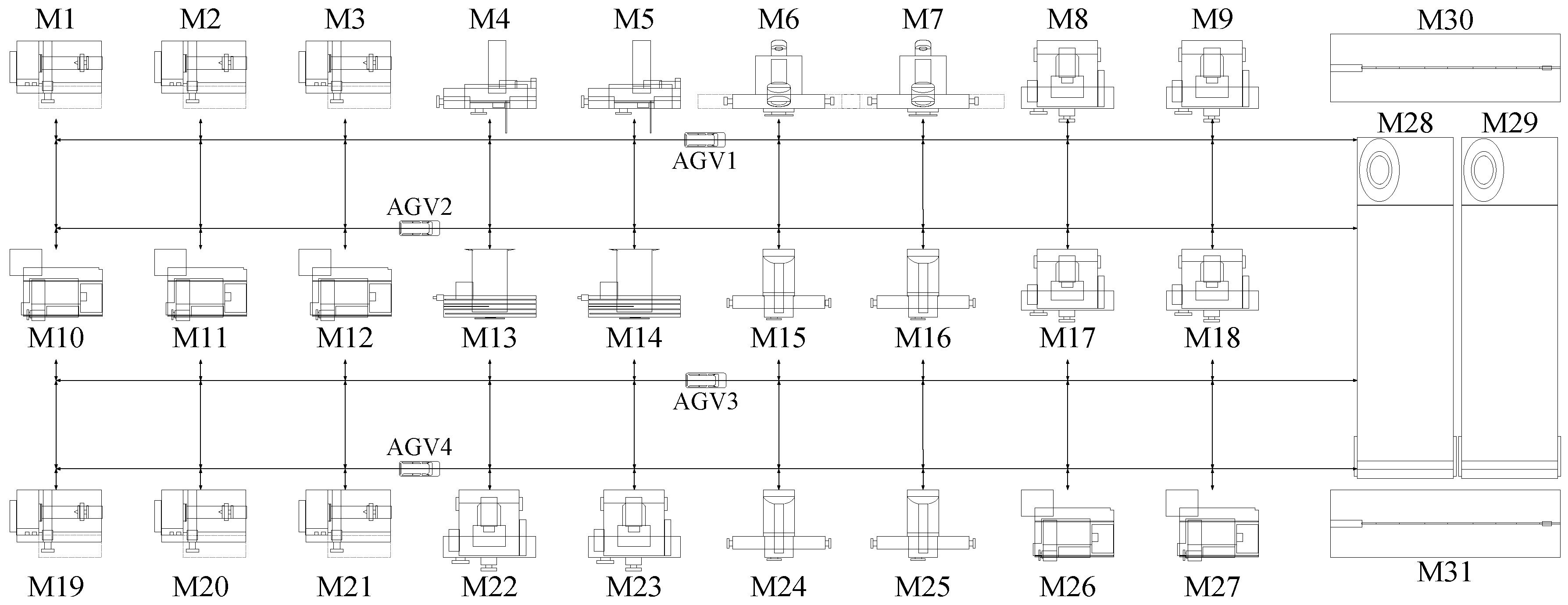
For the ease of understanding, Figure 1 is taken as an example to illustrate the process. As shown in Figure 1, the bearing production shop adopts a mixed U-shaped factory layout and consists of 27 processing machines, 2 assembly machines, 2 quality inspection machines, and 4 AGVs, which are divided into an inner ring production line M₁–M₉, an outer ring production line M₁₀–M₁₈, a roller production line M₁₉–M₂₇, and assembly lines M₂₈ and M₂₉. There are new jobs and maintenance jobs, including inner rings, outer rings, and roller parts; each job has one or more operations, and each operation corresponds to an optional set of machines. The whole process is transported by the AGV, and the product assembly is completed by the assembly machine. Taking the new inner ring component (J₁) as an example, first, M₁ is selected for processing. The quality inspection is carried out after the completion. If the quality inspection of J₁ fails, M₁ is selected for reworking processing. Then, M₅–M₇–M₇–M₉ are selected successively for processing and quality inspection, and the assembly machine (M₂₉) is used to assemble them. After the assembly is completed, the quality inspection will be carried out again. If the quality inspection fails, M₇ should be selected for reworking processing again. After the processing is completed, the quality inspection will be carried out for the next time, until all the production tasks are completed. According to the transportation rules, AGV1–AGV2–AGV1–AGV1–AGV2–AGV2–AGV1 is selected successively for transportation. Through the proper arrangement of the processing, transportation, and assembly for all the tasks, an energy-efficient re-entrant manufacturing process in the bearing production shop is achieved.

2.3. Assumptions

(1)

The shop layout, process parameters, machine parameters, and other information are known;

(2)

At time 0, all the jobs and machines are ready;

(3)

Each machine can only process one job at a certain moment, and one job can only be processed on one machine at a certain moment;

(4)

Once the processing and transportation begin, interruption and preemption are not allowed;

(5)

There is no priority between different jobs;

(6)

AGV transportation cannot exceed the maximum load; AGVs should be driven in accordance with the specified area of the route; the AGVs’ initial positions are at the initial machine, and the first process of the job does not involve any transportation;

(7)

The constraints of the shop buffer zone, storage, and other links are not considered;

(8)

The influence of interference factors, such as machine and AGV failures, are not considered;

(9)

After the system reconfiguration, the operation times of the tool, fixture, and base surface are fixed, and the system recovers after the completion;

(10)

The incline lift time, quality inspection time, and other factors of the manufacturing system are ignored, and the performance parameters of all the machines, AGVs, and tools after the reconfiguration are unchanged.

2.4. Parameter Settings

According to the above information, relevant parameters and variable definitions are shown in

Table 1. Parameter information table.

Notation	Description	Notation	Description
n	The number of jobs	$t_k^{id}$	The standby time of machine k
N	Job assembly {i ∈ (1, 2, …, n)}	Sijk	The start time for Oij on machine k
m	The number of machines	Fijk	The end time for Oij on machine k
M	Machine assembly {k ∈ (1, 2, …, m)}	$t_k^{or}$	The system restoration time of machine k
Oij	The jth operation of job i	$t_k^{es}$	The tool-empty-cutting time of machine k
h	The number of AGVs	$t_k^{is}$	The fixture replacement time of machine k
H	AGV assembly {h ∈ (1, 2, …, H)}	$t_h^{lts}$	The start time of AGV h’s loaded transportation
w	The number of assembly machines	$t_h^{lt}$	The AGV h’s load transportation time
W	Assembly machine assembly {w ∈ (1, 2, …, W)}	$t_h^{lte}$	The end time of AGV h’s loaded transportation
$e_k^{pt}$	The preheating power of machine k	$t_h^{ets}$	The start time of AGV h’s unloaded transportation
$e_k^{ct}$	The cutting power of machine k	$t_h^{et}$	The AGV h’s empty transportation time
$e_k^{id}$	The standby power of machine k	$t_h^{ete}$	The end time of AGV h’s unloaded transportation
$e_k^{or}$	The system restoration power of machine k	$t_h^{aw}$	The AGV h’s waiting time
$e_k^{is}$	The fixture replacement power of machine k	$t_h^{hd}$	The AGV h’s handling time
$e_k^{es}$	The tool-empty-cutting power of machine k	$t_i^{as}$	The assembly time of job i
$e_h^{ltsv}$	The load transportation power of AGV h	$t_w^{ass}$	The start time of assembly machine w
$e_h^{etsv}$	The unloaded transportation power of AGV h	$T_k^a$	The usage cycle of a single diamond pen
$e_h^{wt}$	The standby power of AGV h	Ha	The weight of a single diamond pen
$e_h^{agvhi}$	The handling power of AGV h	$T_k^F$	The usage cycle of the grinding fluid
$e_w^{as}$	The working power of assembly machine w	$N_k^F$	The periodic usage of the grinding fluid
ea	The auxiliary system power	Fe	The electricity’s carbon emission factor
$t_k^{pt}$	The start of the preheating time of machine k	Uh	The AGV h’s maximum load capacity
$t_{ijk}^{ct}$	The cutting time of operation Oij on machine k	Ni	Repair job i type
Xijk	Operation processing decision variables. If operation Oij selects machine k for processing, its value is 1; otherwise, it is 0.
Yijh	Decision variables for job transportation. If operation Oij selects machine h for transportation, its value is 1; otherwise, it is 0.
Ziw	Decision variables for job assembly. If job i is selected for assembly by assembly-machine w, its value is 1; otherwise, it is 0.

.

2.5. Model Formulation

2.5.1. The Makespan Function

The makespan refers to the maximum value of the completion time for the last job to complete the production, and the job needs to go through processing, transportation, and other links before assembly, specifically, as follows:

The makespan function

$$C_{max}=max{\displaystyle \sum _{k=1}^m{\displaystyle \sum _{w=1}^w{\displaystyle \sum _{h=1}^h{\displaystyle \sum _{i=1}^n{\displaystyle \sum _{j=1}^{q_i}\left[t_{ijk}^{ct}+\left(t_h^{lt}+t_h^{et}+t_h^{aw}\right)+\left(t_w^{ase}-t_w^{ass}\right)\right]}}}}}$$

(1)

2.5.2. Total Carbon Emission Function

Relevant studies have confirmed that in job shop scheduling problems, machines are usually divided into four states: on–off, standby, working, and idle [28]. Therefore, combined with the impacts of processing links and transportation links, and the constraints of quality inspection links, some adjustments and optimizations are made to divide the total carbon emission sources into eight links: Machine-preheating carbon emissions, job-cutting and -assembly carbon emissions, machine standby carbon emissions, fixture replacement (installation and disassembly) carbon emissions, system restoration carbon emissions, tool-empty-cutting carbon emissions, auxiliary carbon emissions, and AGV transport carbon emissions. The details are as follows:

(1)

Machine-preheating carbon emissions

The machine needs to be preheated before starting to work so that it can better cut, grind, and perform other operations; the machine will consume energy when preheating, and the entire production process of the machine is only preheated once. The calculation is as follows:

$$E_{pt}={\displaystyle \sum _{k=1}^m{\displaystyle \sum _{i=1}^n{\displaystyle \sum _{j=1}^{q_i}(e_k^{pt}\times t_k^{pt}(X_{ijk})\times F_e)}}}$$

(2)

(2)

Job-cutting and -assembly carbon emissions

Job-cutting and -assembly are the main production processes of machine processing and assembly. Once the machine starts working, it is not allowed to be interrupted. The calculations of the job-cutting and -assembly carbon emissions are as follows:

$$E_{ct1}={\displaystyle \sum _{k=1}^m{\displaystyle \sum _{i=1}^n{\displaystyle \sum _{j=1}^{q_i}(e_k^{ct}\times t_k^{ct}(X_{ijk})\times F_e)}}}$$

(3)

$$E_{ct2}={\displaystyle \sum _{w=1}^w{\displaystyle \sum _{i=1}^n{\displaystyle \sum _{j=1}^{q_i}(e_w^{as}\times t_w^{as}(Z_{iw})\times F_e)}}}$$

(4)

$$E_{ct}=E_{ct1}+E_{ct2}$$

(5)

(3)

Machine standby carbon emissions

The machine standby time is the interval for the machine to wait for subsequent tasks after the current task is completed. The standby carbon emissions of the machine are calculated as follows:

$$E_{id}={\displaystyle \sum _{k=1}^m{\displaystyle \sum _{i=1}^n(e_k^{id}\times t_k^{id}\times F_e)}}$$

(6)

(4)

Fixture replacement (installation and disassembly) carbon emissions

When the machine starts working, different types of jobs need to be installed and corresponding fixtures disassembled, and the carbon emissions of the fixture replacement are calculated as follows:

$$E_{is}={\displaystyle \sum _{k=1}^m{\displaystyle \sum _{i=1}^n{\displaystyle \sum _{j=1}^{q_i}(e_k^{is}\times t_k^{is}(X_{ijk})\times F_e)}}}$$

(7)

(5)

System restoration carbon emissions

According to the concept of the reconfigurable manufacturing system (RMS), when the manufacturing system is reconfigured, the system performance will have a certain recovery time [29]. Combined with the characteristics and constraints of the proposed model, according to the information of jigs and tools required by the machine, the carbon emissions generated by the manufacturing system restoration are calculated as follows:

$$E_{or}={\displaystyle \sum _{k=1}^m{\displaystyle \sum _{i=1}^n{\displaystyle \sum _{j=1}^{q_i}(e_k^{or}\times t_k^{or}(X_{ijk})\times F_e)}}}$$

(8)

(6)

Tool-empty-cutting carbon emissions

At the beginning of the processing, the machine will have a period of tool-empty-cutting time, and the carbon emissions generated by the tool empty cutting are calculated as follows:

$$E_{es}={\displaystyle \sum _{k=1}^m{\displaystyle \sum _{i=1}^n{\displaystyle \sum _{j=1}^{q_i}(e_k^{es}\times t_k^{es}(X_{ijk})\times F_e)}}}$$

(9)

(7)

Auxiliary carbon emissions

In the production process, auxiliary systems, such as lighting, ventilation, and air conditioning, are needed, and the carbon emissions by these parts are calculated as follows:

$$E_a=e_a\times C_{max}\times F_e$$

(10)

(8)

AGV transport carbon emissions

AGV transportation carbon emissions mainly come from its transportation, waiting, and other states, and the calculation is as follows:

$$\begin{array}{l}{E}_{ts}=E_{ets}+E_{wt}+E_{up}\\ ={\displaystyle \sum _{h=1}^h{\displaystyle \sum _{i=1}^n{\displaystyle \sum _{j=1}^{q_i}\left[(e_h^{ltsv}\times t_h^{lt}+e_h^{etsv}\times t_h^{ets})\times Y_{ijh}\times F_e+e_h^{wt}\times t_h^{aw}\times Y_{ijh}\times F_e+e_h^{agvhi}\times t_h^{hd}\times Y_{ijh}\times F_e\right]}}}\end{array}$$

(11)

Based on the above analysis, it is concluded that the total carbon emission function is as follows:

$$E_{to}=E_{pt}+E_{ct}+E_{id}+E_{is}+E_{or}+E_{es}+E_a+E_{ts}$$

(12)

2.5.3. The Waste Emission Function

In the production process of high-performance bearings, auxiliary resources, such as the grinding fluid, diamond pen, and lubrication fluid, need to be used, and certain wastes will be generated in the using process. After the simplification and summary, the grinding fluid and diamond pen are selected as waste discharge indicators in this problem. According to the information, such as the service cycle, machine model, and service time, the waste emission function is calculated as follows:

The grinding fluid

$$W_{\mathrm{e}}={\displaystyle \sum _{k=1}^m{\displaystyle \sum _{i=1}^n{\displaystyle \sum _{j=1}^{q_i}(\frac{t_{ijk}^{ct}}{T_k^F}\times N_k^F(X_{ijk})\times M_k)}}}$$

(13)

The diamond pen

$$W_a={\displaystyle \sum _{k=1}^m{\displaystyle \sum _{i=1}^n{\displaystyle \sum _{j=1}^{q_i}(\frac{t_{ijk}^{ct}}{T_k^a}\times H_a)}}}$$

(14)

2.5.4. The integrated Optimization Model

Based on the above analysis, with the makespan as the economic index and the total carbon emissions and waste emissions as the green index, the mathematical model and constraint conditions are established. The details are as follows:

The objective function

$$MinZ=CT+CE+CW$$

(15)

The makespan

$$CT=min(T_i)$$

(16)

Total carbon emissions

$$CE=min{E}_{to}$$

(17)

The waste emissions

$$CW=min(W_e+W_a)$$

(18)

Constraints:

${\displaystyle \sum _{k=1}^m{X}_{ijk}=1}$ means that only one machine can be selected for one process at a time.

${\displaystyle \sum _{n=1}^i{X}_{ijk}=1}$ means that each machine can only process one job at a time.

$F_{ijk}-S_{ijk}=t_{ijk}^{ct}$ means that the job cannot be interrupted once it has started processing.

$S_{ijk}\ge F_{i(j-1)k}$ represents the operation constraint of the new job.

$N{S}_{ijk}\ge N{F}_{i(j-1)k}$ represents the operation constraint of the maintenance job.

${\displaystyle \sum _{k=1}^m{X}_{ijk}=1}$. ${\displaystyle \sum _{h=1}^h{Y}_{ijh}=1}$. ${\displaystyle \sum _{w=1}^w{Z}_{iw}=1}$ means that only one machine can be selected for all the tasks at a time and belongs to the optional machine set.

${\displaystyle \sum _{k=1}^m{X}_{ij}^k=1}$ means the machine selection constraints for the reconstituted production line.

${\displaystyle \sum _{t=1}^t{{\displaystyle X}}_{ij}^k}=1$ means that all the jobs must be processed and can be processed only once.

$S_{ijk}\ge 0,F_{ijk}\ge 0,t_{ijk}^{ct}\ge 0,t_h^{lte}\ge t_h^{lts}$ means that the start time, end time, processing time, and transportation time of any task are not less than 0.

${\displaystyle \sum _{i=1}^n{\displaystyle \sum _{j=1}^m{X}_{ijk}}\le }{U}_h$ means the constraint on the AGV load capacity.

${\displaystyle \sum _{h=1}^h{Y}_{ijh}=1}$ means that the transportation task of any job at a time is completed by a maximum of one transport machine.

$F_{ij}+t_h^{lt}\le S_{i(j+1)}$ indicates that the start time of the transportation task must not be earlier than the sum of the end time and processing time of the last process of the job.

${\displaystyle \sum _{n=1}^i{Z}_{iw}=1}$ means that each assembly machine can only assemble one job at a time.

$F_{ijk}+t_h^{lt}\le t_w^{ass}$ indicates that the assembly cannot begin until corresponding parts have been transported.

3. Solution Framework and Algorithm Flow

3.1. Machine Restructuring Pretreatment

The processing of the job usually corresponds to different types of manufacturing units, and each manufacturing unit of the manufacturing system usually includes more than one machine. The selection and clustering of machine combinations according to the machine selection flexibility of the machining process can effectively improve the efficiency of the system reconfiguration and production scheduling [30]. Because of the complexity of the process and the different system functions of manufacturing units, the parallel machine selection of different jobs in the job family is also different. If all the selected machines are arranged in the same manufacturing unit for the production, it will cause problems, including staggered process routes, interrupted production lines, and unequal machine loads. Based on the above analysis, the concepts of the set of the longest common machine routes (SLCMR) and the set of the shortest recombination machine combinations (SSRMC) are proposed in this paper.

SLCMR is the set of the longest machine selection sub-routes set between different jobs with the same process or the same function. SSRMC is the machine selection set that refers to taking SLCMR as the core by adding the corresponding machine combinations of non-similar processes between each job. SLCMR and SSRMC can effectively reflect the logic and essence of the production line’s machine structure, so the analysis of the production line’s machine recombination set can effectively improve the operation efficiency and avoid production line interruptions, resource waste, and other problems.

To facilitate an understanding, an example to illustrate the meaning of the above concepts is shown in

Table 2. Job information table to illustrate the concept of SLCMR and SSRMC.

Job Type		Operation	M1	M2	M3	M4	M5	M6	M7	M8
New job	J1	O11	2	2
		O12			2	3
	J2	O21	1	2
		O22			3	4
		O23					4	5
	J3	O31	1	2
		O32			2	3
		O33							6	7
Maintenance job	J4	O41	1	2
		O42			1	1
		O43					1	2
	J5	O51	2	3
		O52			1	2
	J6	O61	1	2
		O62			2	3
		O63							2	3

. In Table 2, the job information is given. Taking jobs J₁ and J₄ as examples, J₁ has two operations, and each operation corresponds to two parallel machines, so the job has a total of 2 × 2 = 4 machine selection route sets. J₄ has three operations, and each operation corresponds to two parallel machines, so the job has a total of 2 × 2 × 2 = 8 machine selection route sets. The same method is used for the rest of the jobs. Therefore, when adjusting the machine structure of the production line, according to the definitions of the SLCMR and SSRMC, taking maintenance jobs J₄, J₅, and J₆ as examples, it can be concluded that for maintenance jobs, SLCMR = {1, 3}, {1, 4}, {2, 3}, or {2, 4}, and SSRMC = {1, 3, 5, 7}, {1, 3, 5, 8}, {1, 3, 6, 7}, {1, 3, 6, 8}, {1, 4, 5, 7}, {1, 4, 5, 8}, {1, 4, 6, 7}, {1, 4, 6, 8}, {2, 3, 5, 7}, {2, 3, 5, 8}, {2, 3, 6, 7}, {2, 3, 6, 8}, {2, 4, 5, 7}, {2, 4, 5, 8}, {2, 4, 6, 7}, or {2, 4, 6, 8}. The same method is true for corresponding new jobs J₁, J₂, and J₃.

3.2. Algorithm Flow

In this paper, the proposed integrated optimization model involves multi-dimensional and multi-variable optimizations, including machine selection flexibility, transportation path selection flexibility, process flexibility, and system recombination flexibility. To solve this multi-dimensional and multi-variable complex integrated optimization problem, a multi-objective hybrid optimization algorithm, based on a neighborhood local search (MOOA-LS), is proposed. The MOOA-LS algorithm combines the hybrid optimization algorithm with the neighborhood search strategy and adopts the probability-based neighborhood search strategy to ensure that the solution after the crossover operation meets the taboo table rules to strengthen the algorithm’s ability to jump out of the local optimization, expand the search scope of the understanding, and avoid the premature convergence of the algorithm. The overall flow of the algorithm is shown in Figure 2.

3.2.1. Encoding and Decoding

To improve the efficiency and reduce the difficulty of the calculation, the four-segment encoding method is used in this section. The encoding consists of four parts: machine assignment, operation sequencing based on the type of the job, machine selection, and AGV selection. The information in

Table 3. Job information table to illustrate the algorithm flow.

Job Type		Operation	Machine/Time	AGV
New job	J1	O11	M1/3, M2/4	AGV1, AGV2, AGV3
		O12	M3/3, M4/5	AGV1, AGV2
		O13	M5/7, M6/8, M7/7	AGV1, AGV2, AGV3
	J2	O21	M1/5, M2/6	AGV1, AGV2
		O22	M3/9, M4/8	AGV1, AGV2, AGV3
Maintenance job	J3	O31	M1/2, M2/3	AGV1, AGV2, AGV3
		O32	M3/3, M4/4	AGV1, AGV2, AGV3
	J4	O41	M1/1, M2/2	AGV1, AGV2
		O42	M3/3, M4/4	AGV1, AGV2, AGV3
		O43	M5/5, M6/6, M7/6	AGV1, AGV2

is taken as an example to illustrate this.

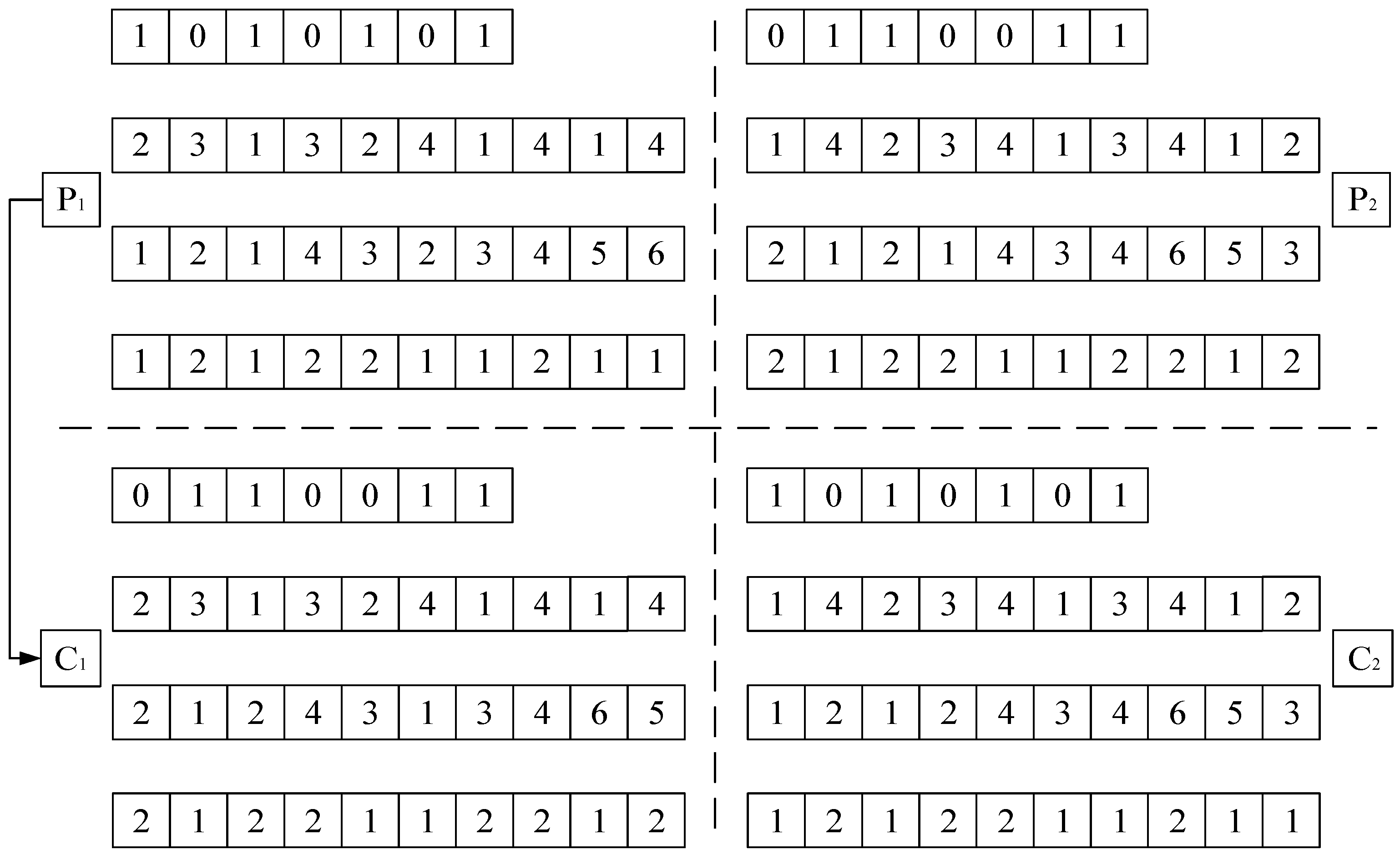
Figure 3 shows an example of the encoding scheme; as is shown, the first part of the chromosome is the machine assignment to select the corresponding machine for all the jobs and generate the corresponding production line’s machine combination. Each gene is represented by a real number; the production line’s machine selection for new jobs is set at 1, and the production line’s machine selection for maintenance jobs is set at 0. The second part of the chromosome is the operation sequencing based on the type of the job to generate the operation sequencing of all the jobs. Each gene is represented by a real number; different job types are represented by different numbers, all the operations of the jobs are randomly arranged, and the number of occurrences of different numbers is equal to the total number of operations of the jobs. The third part of the chromosome is the machine selection. First, judge the type of job, then select the corresponding machine for all the processes according to the corresponding production line’s machine combination and operation sequencing. Each gene is represented by a real number, arranged in sequence according to the sequence order of the operation, and each real number represents the sequence number of the machine selected for the current operation in the optional machine set. The fourth part of the chromosome is the AGV selection; each gene is represented by a real number, arranged according to the operation sequence and machine selection. Each real number represents the sequence number of the AGV selected by the current operation in the optional AGV set.

Based on the above encoding method, the decoding process of a specific chromosome is implemented is as follows:

Step 1: Generate a certain number of chromosomes based on the above encoding steps;

Step 2: Select a chromosome randomly, scan each gene in the chromosome from top to bottom, and select a process randomly. First, determine the corresponding job type and production line. Then, determine the corresponding machine and AGV;

Step 3: Select all the chromosomes to obtain the job type, processing time, machine selection, and AGV selection of all the operations;

Step 4: Repeat the above steps to complete the decoding.

3.2.2. Population Initialization

At the beginning of the algorithm, according to the updated job and machine state, the initial population (P) is constructed by random initialization.

3.2.3. Fast Non-Dominated Sorting and Congestion Calculation

To ensure the survival of the fittest individual populations, the algorithm adopts the method of the tournament selection for fast non-dominated sorting. First, the solutions are sorted according to the fitness function of the individual, and the solutions with better fitness are selected as the parent chromosome. Then, the crowding distance of the solutions with the same fitness is calculated, and the choices are made successively to obtain the elite parent chromosome.

3.2.4. Crossover Operation

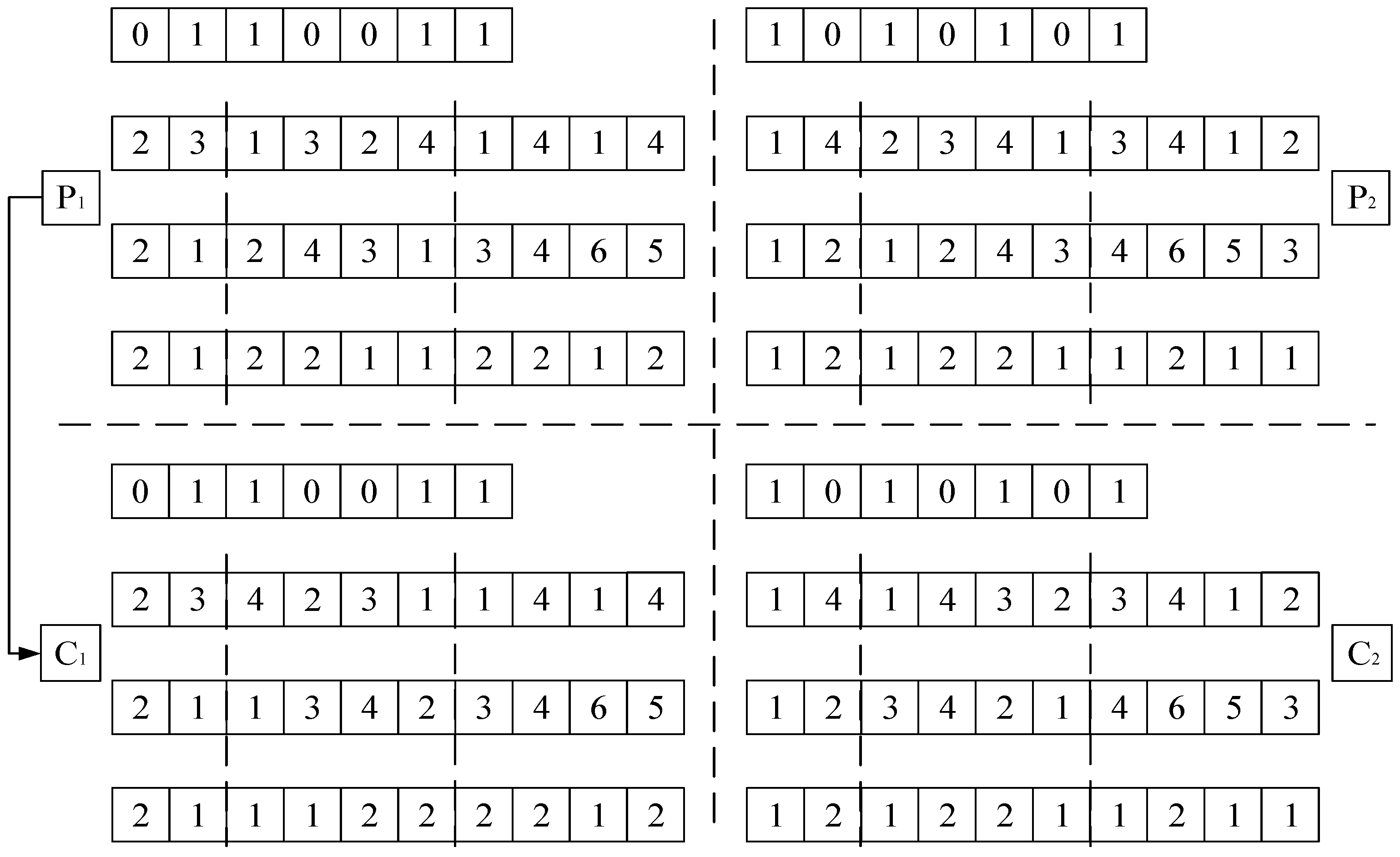
In the four-part encoding, the machine assignment plays a decisive role in the subsequent operation. Therefore, this paper draws on the ideas of uniform crossover [31] and single point crossover [32] to improve the crossover operation. As shown in Figure 4, the specific steps are as follows: the parent chromosomes (P₁ and P₂) are randomly generated, the machine assignment encoding parts of P₁ and P₂ are exchanged, and the operation sequencing is unchanged. Then, according to the newly generated machine assignment, the new machine selection and AGV selection are generated again to obtain two new chromosomes (C₁ and C₂) and finally complete the crossover operation.

3.2.5. Mutation Operation

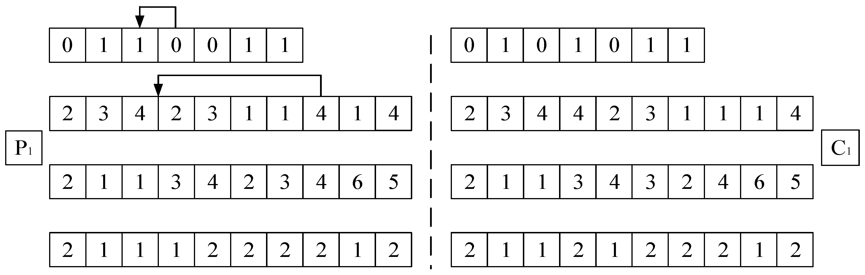
According to the four parts of the encoding, in the process of the mutation operation, it mainly focuses on the machine assignment and operation sequencing parts, and the machine selection and AGV selection are subsequently changed, as shown in Figure 5.

To ensure the effectiveness of the chromosome, an improved exchange mutation method is adopted in the machine assignment’s mutation operation. First, randomly select a gene segment of the same machine selection set in a parent chromosome. Then, swap the machine numbers of the two positions to regenerate a new chromosome and complete the machine-assigned variation. Then, the improved insertion mutation mode is adopted in operation-sequencing mutation operations based on the premise for ensuring the generation of feasible solutions. First, a gene fragment in the process sequence of the parent chromosome is randomly selected. Then, under the premise for ensuring the process sequence constraint of the job, another position of the chromosome is randomly inserted to generate a new chromosome and complete the variation in the operation sequencing. The AGV selection mutation is the same as the machine selection mutation. For example, when carrying out machine selection mutations, because of the optional machine sets in each process, a position on the chromosome is first randomly selected. Then, one machine is selected from the optional machine set of the process to replace the original machine and complete the machine selection mutation.

3.2.6. Taboos and Amnesty Rules

The taboo table is designed to control the population search’s precision after crossover operations, including the taboo table’s length and amnesty criteria. First, the length of the taboo table is set at 20, and the obtained chromosomes are placed in the taboo table when the chromosomes are crossed over. If the chromosomes match, they are regarded as daughter chromosomes; if not, they are removed. When the taboo table is full, the first-in first-out principle is followed to remove the taboo fitness difference solutions and release space for new solutions. Then, by comparing the fitness values of the current solution and the taboo table, the solutions with good fitness are amnestied, and the solutions that meet the amnesty criteria are added to the taboo table. Finally, the taboo table is updated to obtain a new progeny chromosome population, which is convenient for the subsequent local neighborhood optimization.

3.2.7. Neighborhood Search Strategy

Because the job has operational flexibility, there are optional machine sets during processing, and the difference in machine selection will lead to changes, such as the AGV waiting time, transportation time, and transportation path, that, in turn, affect the job operation sequence. Therefore, after the machine combination of the production line is determined, under the premise for satisfying the machine allocation constraints, the new domain search strategy can be proposed to optimize the process ordering, machine selection, and AGV allocation to improve the whole production process. As shown in Figure 6, the specific steps are as follows:

Step 1: After completing the crossover operation, select the generated offspring chromosome as the new parent chromosome;

Step 2: Randomly intercept a part of the operation sequencing chromosome, and under the premise for meeting the process constraints, reorder the fragment to generate a new offspring chromosome, and transform the machine selection and AGV selection chromosomes;

Step 3: The probability P_a determines whether to accept the individual as a result of the neighborhood search. If yes, accept. If no, return to step 2;

Step 4: Repeat the above steps to update the taboo table’s status.

4. Case Study

To verify the effectiveness of the proposed model and algorithm, experimental design and analysis are carried out for a bearing production shop. The experimental design and analysis consist of three parts in this section: (1) a case analysis of a bearing production shop, (2) a comparative analysis with other algorithms, and (3) data testing at different data scales.

4.1. Case Background

The bearing production shop mainly produces high-performance military-series precision bearings with high product quality standards and harsh performance indicators, and there are often various reworking and repair problems caused by unqualified product quality inspections in the production process. The bearing production shop consists of an inner ring production area, an outer ring production area, a roller production area, an assembly area, and a quality inspection area and mainly produces inner rings, outer rings, and roller parts. All the parts are assembled after processing, and the AGV is responsible for transportation. All the jobs need to go through processing, transportation, assembly, and quality inspection steps until the last product is completed. To facilitate this study, it is stipulated that the re-entrant process is randomly generated, the maximum number of re-entrant times is 3 times, and the information is scientifically and reasonably supplemented and adjusted, including the process flow, machine parameters, and workshop layout.

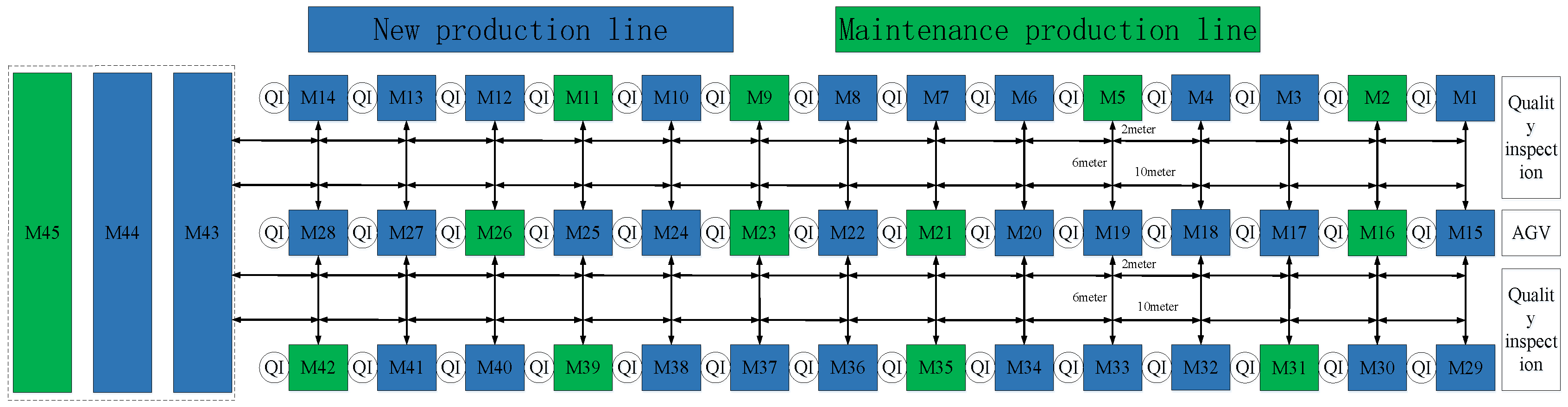
The experiment takes five types of bearings as examples, namely, 313XC, 315XC, 322XC, 350X, and 352X types of bearings. The machine parameter information is shown in

Table 4. Machine information sheet.

Machine Group Number	Machine Group Name	Rated Power/kw	Idle Power/kw	Preparation Time/h	System Restoration Time/h
M1, M2, M15, M16	Double end grinding machine	88	8	0.2	0.05
M3, M4, M11, M12, M23, M24, M25	Internal grinder	36	5	0.2	0.05
M5, M6	Inner ring track grinding machine	12	2	0.2	0.05
M7, M8	Internal track grinding machine	76	7	0.2	0.05
M9, M10	Inner ring edge grinding machine	76	7	0.2	0.05
M13, M14	Nc-tapered roller bearing inner ring superfinishing machine	45	5	0.2	0.05
M17, M18, M21, M22	External cylindrical grinding machine	45	5	0.2	0.05
M19, M20	Outer ring double track grinding machine	50	5	0.2	0.05
M26, M27, M28	Nc-tapered roller bearing outer ring superfinishing machine	45	5	0.2	0.05
M29, M30, M31	Surface centerless grinding machine	78	7	0.2	0.05
M34, M35	Roller ball base superfinishing machine	45	5	0.2	0.05
M32, M33, M36, M37	Conical roller centerless grinding machine	36	5	0.2	0.05
M38, M39	Centerless outside diameter grinding machine	45	5	0.2	0.05
M40, M41, M42	Superfinishing machine	22	3	0.2	0.05
M43, M44, M45	Assembling machine	100	10	0.2	0.05

, including the machine groups’ names, rated powers, and idle powers.

Table 5. AGV information sheet.

AGV Type	Rated Power/kw	Idle Power/kw	Load Power/kw	Unload Power/kw	Speed (km/h)	Single Transport Time/min
AGV1	20	2.1	20	15	3.6	3
AGV2	25	2.3	25	20	5.4	3
AGV3	30	2.5	30	25	7.2	3

gives the AGV information, including the rated power, idle power, and load power. The processing of bearings mainly includes grinding two ends, sharpening the outside diameter of the flange, end grinding large flanges, and the superfine grinding of the inner raceway and large flanges. The processing time mainly includes the fixture installation time, cutting time, and fixture disassembly time. The cutting processing is completed by M₁–M₄₂; for space reasons, only the bearing processing information of 313XC and 350X is given, as shown in

Table 6. New job information sheet.

Job	Operation	Job Process	Machine	Cutting Time/h	Fixture Installation Time/Fixture Disassembly Time (h)
313XC inner ring 1	O11	Grinding two ends	M1, M2	0.18, 0.2	0.01/0.01
	O12	Initial grinding of the inner raceway, large flange, and inner diameter	M3, M4	0.3, 0.35	0.01/0.01
	O13	Sharpening the outside diameter of the flange	M5, M6	0.08, 0.06	0.01/0.01
	O14	Final grinding of the inner raceway	M7, M8	0.12, 0.1	0.01/0.01
	O15	End grinding of the large flange	M9, M10	0.16, 0.15	0.01/0.01
	O16	Final grinding of the inside diameter	M11, M12	0.15, 0.12	0.01/0.01
	O17	Superfine inner raceway, large flange	M13, M14	0.1, 0.12	0.01/0.01
313XC inner ring 2	O21	Grinding two ends	M1, M2	0.2, 0.22	0.01/0.01
	O22	Initial grinding of the inner raceway, large flange, and inner diameter	M3, M4	0.28, 0.3	0.01/0.01
	O23	Sharpening of the outside diameter of the flange	M5, M6	0.1, 0.08	0.01/0.01
	O24	Final grinding of the inner raceway	M7, M8	0.15, 0.12	0.01/0.01
	O25	End grinding of the large flange	M9, M10	0.18, 0.15	0.01/0.01
	O26	Final grinding of the inside diameter	M11, M12	0.16, 0.15	0.01/0.01
	O27	Superfine inner raceway, large flange	M13, M14	0.15, 0.18	0.01/0.01
313XC outer ring	O31	Grinding two ends	M15, M16	0.1, 0.13	0.01/0.01
	O32	Initial grinding of the outside diameter	M17, M18	0.08, 0.06	0.01/0.01
	O33	Initial grinding of the outside raceway	M19, M20	0.13, 0.12	0.01/0.01
	O34	Final grinding of the outside diameter	M21, M22	0.15, 0.18	0.01/0.01
	O35	Final grinding of two outer raceways	M23, M24, M25	0.16, 0.18, 0.2	0.01/0.01
	O36	Superfine outer raceway	M26, M27, M28	0.2, 0.22, 0.25	0.01/0.01
313XC roller	O41	Rough face grinding	M29, M30, M31	0.2, 0.24, 0.25	0.01/0.01
	O42	Rough grinding rolling surface	M32, M33	0.1, 0.12	0.01/0.01
	O43	Grinding the ball base	M34, M35	0.1, 0.13	0.01/0.01
	O44	Finely grinding the rolling surface	M36, M37	0.1, 0.12	0.01/0.01
	O45	Final grinding of the rolling surface	M38, M39	0.06, 0.08	0.01/0.01
	O46	Superfine rolling surface	M40, M41, M42	0.08, 0.1, 0.11	0.01/0.01

and

Table 7. Maintenance job information sheet.

Job	Operation	Job Process	Machine	Cutting Time/h	Fixture Installation Time/Fixture Disassembly Time (h)
350X inner ring 1	O11	Grinding two ends	M1, M2	0.12, 0.13	0.01/0.01
	O13	Sharpening the outside diameter of the flange	M5, M6	0.08, 0.1	0.01/0.01
	O16	Final grinding of the inside diameter	M11, M12	0.1, 0.12	0.01/0.01
350X inner ring 2	O21	Grinding two ends	M1, M2	0.1, 0.12	0.01/0.01
	O23	Sharpening the outside diameter of the flange	M5, M6	0.06, 0.08	0.01/0.01
	O25	End grinding of the large flange	M9, M10	0.08, 0.1	0.01/0.01
350X outer ring	O31	Grinding two ends	M15, M16	0.1, 0.12	0.01/0.01
	O35	Final grinding of two outer raceways	M23, M24, M25	0.12, 0.15, 0.16	0.01/0.01
	O36	Superfine outer raceway	M26, M27, M28	0.18, 0.2, 0.22	0.01/0.01
350X roller	O41	Rough face grinding	M29, M30, M31	0.16, 0.18, 0.2	0.01/0.01
	O45	Final grinding of the rolling surface	M38, M39	0.1, 0.12	0.01/0.01
	O46	Superfine rolling surface	M40, M41, M42	0.08, 0.1, 0.11	0.01/0.01

, respectively. The assembly of the bearings is completed by M₄₃–M₄₅, and the value of the assembly time (t) ranges from 0.2 to 0.25 h. In the calculation of carbon emissions, the carbon emissions generated by electric energy need to be converted by the carbon emission factor, and the value is 0.6747 kg-CO₂/kw·h. In this experiment, waste emissions are mainly generated by the grinding fluid and diamond pen. The value of the grinding fluid’s cycle usage (w) ranges from 0.25 to 0.5 kg, the service cycle is 1 h, the weight of a single diamond pen is 0.3 kg, and the value of a single service time (t) ranges from 15 to 20 h. In addition, the power of auxiliary systems, such as lighting and ventilation, is set at 50 kw. The layout of the production shop is shown in Figure 7, including machine locations and the prescribed route.

4.2. Case Analysis of a Bearing Production Shop

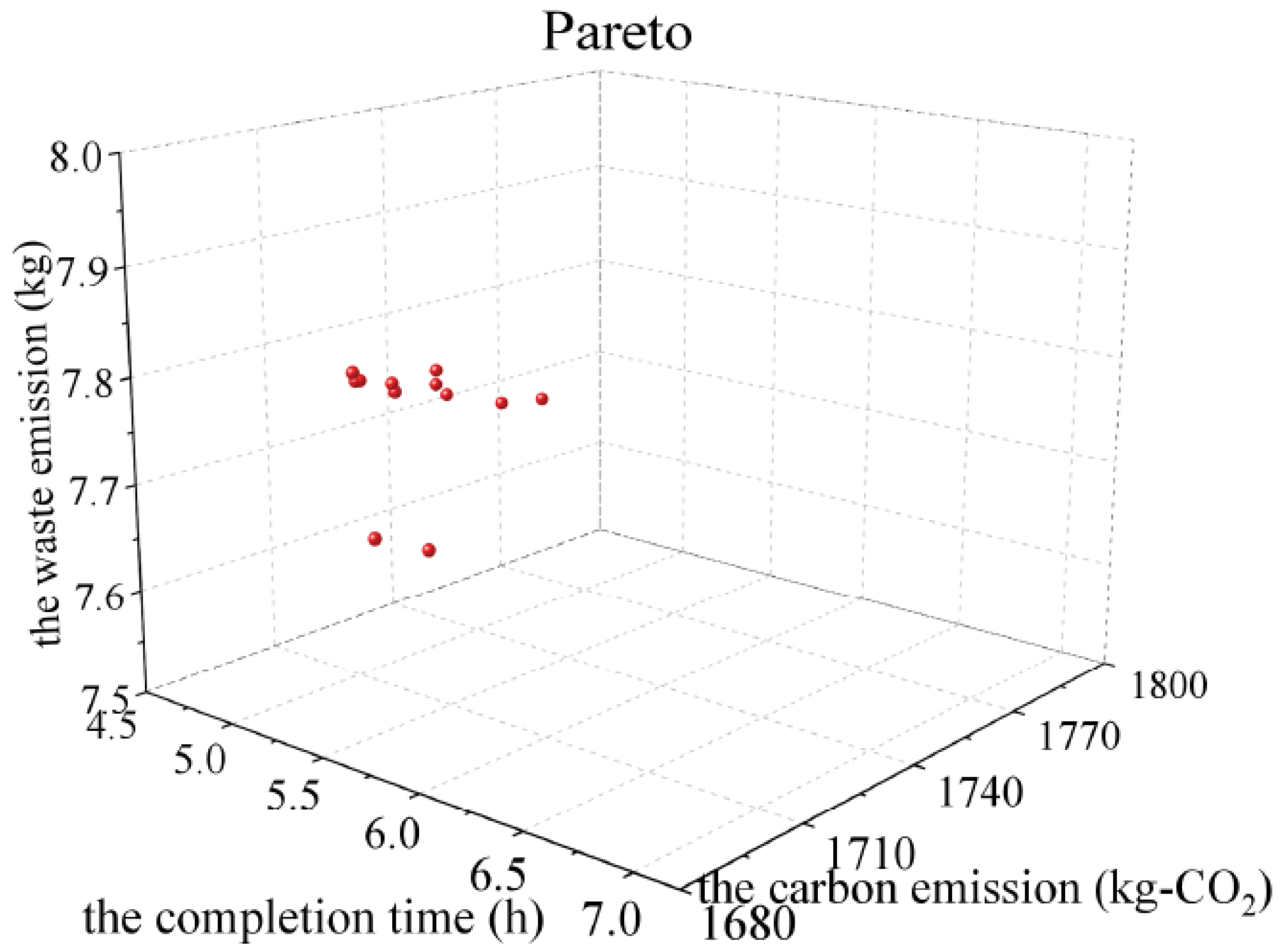
According to the above information, the number of bearing batches for each type is set at 1, the number of AGVs for each type is set at 2, the remaining information is unchanged, and a group of feasible Pareto front solution sets is obtained, as shown in Figure 8. Some selected objective function values are shown in

Table 8. Pareto objective function values.

Serial Number	CT/h	CE/kg-CO2	CW/kg
1	5.10	1742.38	7.73
2	5.18	1749.24	7.73
3	5.02	1731.93	7.75
4	4.98	1731.42	7.77
5	5.44	1695.54	7.68
6	5.54	1703.70	7.66
7	5.19	1702.66	7.80
8	5.19	1702.02	7.81
9	5.20	1703.30	7.80
10	5.23	1710.12	7.78

(10 qualified values are numbered from top to bottom, with two decimal points reserved). For space reasons, the solution with the minimum makespan (serial number 5) is selected from the Pareto front solution sets, and the corresponding scheduling’s Gantt chart is generated by decoding, as shown in Figure 9. The numbers at the front of the Gantt chart represent the job, the numbers at the back represent the process, and different colors represent different types of jobs. The re-entrant information is shown in

Table 9. Re-entrant information table.

Job	Re-entry Operation and Number of Re-Entries
313XC	O14, O15(2), O16, O17, O25, O26, O27, O32, O33, O42, O43
315XC	O13, O16(2), O22, O23, O26, O33, O34, O43, O45(2)
322XC	O13, O16, O26, O27, O32, O33, O43, O46, Assemble
350X	O13, O16(2), O23, O36, O46
352X	O15, O25(2), O34, O46

. The machine combination information of the production line is shown in Figure 10.

In the Pareto frontier’s solution set, serial number 4, serial number 5, and serial number 6 are the solutions with the minimum makespan, minimum total carbon emissions, and minimum waste emissions, respectively. It can be seen that the three objective functions conflict with each other, and it is difficult to reach the optimum at the same time. For example, in the solution with the minimum makespan (serial number 4), its makespan, total carbon emissions, and waste emissions are 4.98 h, 1731.42 kg-CO₂, and 7.77 kg, respectively. The solution with serial number 4 has the best makespan, but its total carbon emissions and waste emissions are inferior, which is because in this scheme, to complete the task as quickly as possible, the job is preferentially allocated to the short-time high-power machines and AGVs, resulting in increases in the total carbon emissions and waste emissions. Compared with the solution with the minimum waste emissions (serial number 6), its makespan, total carbon emissions, and waste emissions are 5.54 h, 1703.70 kg-CO₂, and 7.66 kg, respectively. The solution with serial number 6 has the best waste emissions and better total carbon emissions, but its makespan is the worst, which is because in this scheme, to reduce the total carbon emissions and waste emissions as much as possible, the job is preferentially allocated to the low-power long-time machines, which causes the waiting, processing, and transportation times to be too long, resulting in an increase in the makespan. In the actual production process, to achieve a certain conflict balance between the various objective functions, the decision maker can choose the appropriate scheme according to the actual demand. For example, the solutions corresponding to serial number 7, serial number 8, and serial number 9 not only meet the production efficiency but also reduce the production energy consumption to a certain extent and achieve a good balance among the makespan, total carbon emissions, and waste emissions, which have very important reference values.

In the production planning scheme obtained in this experiment, the load distribution of each machine is relatively balanced, the AGV distribution and path planning are also relatively reasonable, and the re-entrant process is within a reasonable range. When any process needs to be re-entered, using the proposed model and algorithm can adjust the production plan in time, and the machine and AGV can be reasonably allocated to reduce the negative effects of production line stagnation and for planning interruptions caused by process re-entry, all of which can effectively ensure the smooth progress of the production plan.

In addition, it can also be seen, when generating production line machine combinations, that the proposed model and algorithm can make reasonable use of the process, layout, and machine information and reasonably allocate system resources under the premise for minimizing the variation range of manufacturing system resources to meet the production needs of new and maintenance jobs to the greatest extent and realize the collaborative optimization of production balance and system resources.

4.3. Comparative Analysis with Other Algorithms

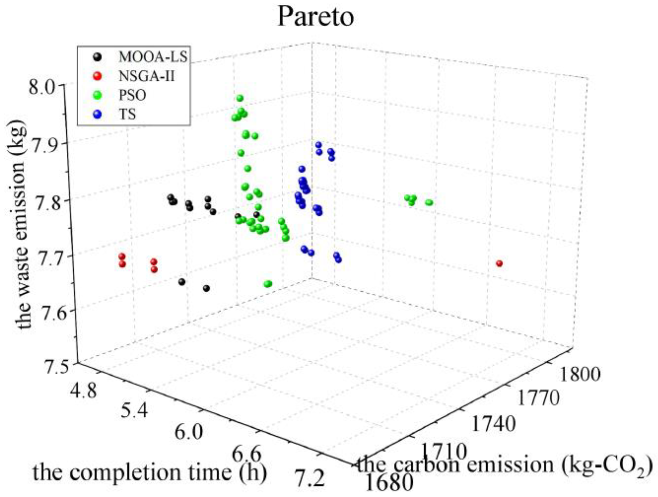
This section sets up an algorithmic comparison. Based on the case data and some modifications, the proposed algorithm is compared with the non-dominated sorting genetic algorithm-II (NSGA-II), particle swarm optimization (PSO), and taboo search algorithm (TS). The data of the above cases are substituted into the solution, and the Pareto front comparison is shown in Figure 11. The comparison of the optimization results is shown in

Table 10. Comparison table of optimization results.

Algorithm	Objective Function	CT/h	CE/kg-CO2	CW/kg
MOOA-LS	CT	4.98	1731.42	7.77
	CE	5.44	1695.54	7.68
	CW	5.54	1703.70	7.66
NSGA-II	CT	4.99	1684.96	7.71
	CE	5.00	1684.64	7.70
	CW	7.13	1789.98	7.68
PSO	CT	5.62	1719.34	7.89
	CE	5.98	1714.79	7.68
	CW	5.98	1715.57	7.68
TS	CT	5.65	1762.06	7.87
	CE	6.06	1727.67	7.82
	CW	6.02	1753.70	7.68

(two decimal points are retained).

Through analysis, it can be seen that in most cases, the Pareto front solution sets obtained by the NSGA-II, PSO, and TS algorithms are dominated by the Pareto front of the MOOA-LS algorithm, and the distribution, uniformity, and convergence of the Pareto front obtained by the MOOA-LS algorithm are superior to those obtained by the comparison algorithms. It shows that the MOOA-LS algorithm can reasonably optimize the machine selection and transportation planning of the process and reduce the idle time to improve the production efficiency. Therefore, it can be concluded that the proposed MOOA-LS algorithm has a better solving performance than other algorithms and can effectively solve the green re-entrant scheduling problem under the reworking interference of bearing products.

4.4. Data Testing at Different Data Scales

Because of the variety of bearing products and large production batches, small-scale data experiments have limitations and cannot reflect the re-entrant production characteristics of bearing products. Therefore, to further verify the feasibility of the proposed model and algorithm in engineering applications, this section conducts data testing at different data scales. Based on the case information, the following conditions are added: Based on the uniform distribution theory, the number of bearing batches for each type is set at N ≈ [1, 10], and the number of AGVs for each type is set at H ≈ [1, 6]; six groups of calculation examples (numbered N01–N06) are randomly generated to carry out data testing at different data scales.

To facilitate this study, some constraints, such as the AGV fault, buffer size, and storage, are not considered; the remaining information remains unchanged. The comparison of the obtained Pareto fronts is shown in Figure 12, and the comparison of the experimental results is shown in

Table 11. Comparison table of optimization results at different data scales.

Algorithm	Objective Function		N01	N02	N03	N04	N05	N06
MOOA-LS	CT	CT/h	7.42	9.10	11.84	15.84	18.73	21.28
		CE/kg-CO2	2435.11	3096.54	4092.81	5578.92	6933.85	8397.06
		CW/kg	11.40	14.63	19.90	27.82	34.40	41.30
NSGA-II	CT	CT/h	7.40	8.94	12.13	16.24	19.14	21.86
		CE/kg-CO2	2481.85	3092.34	4057.64	5628.57	6835.16	8328.77
		CW/kg	11.68	14.57	19.70	27.50	34.53	41.61
PSO	CT	CT/h	7.32	9.22	12.49	16.16	19.58	21.60
		CE/kg-CO2	2442.06	3112.55	4125.92	5685.05	7009.96	8442.57
		CW/kg	11.62	14.92	20.19	27.74	34.69	41.67
TS	CT	CT/h	7.84	9.68	12.41	17.38	19.65	20.77
		CE/kg-CO2	2486.48	3072.13	4063.46	5644.15	7062.49	8269.09
		CW/kg	11.68	14.61	19.70	27.49	34.22	41.46

(taking the solution value of the minimum makespan as an example, two decimal points are retained).

The analysis shows that with the expansion of the data scale, in most examples, the solution quality of the MOOA-LS algorithm is superior to those of the other algorithms in terms of the objective function values and Pareto dominance relationships and convergence. Therefore, it can be further verified that the proposed algorithm is a very competitive algorithm to solve such problems. In practical applications, using the proposed algorithm can effectively improve the production efficiency, reduce environmental pollution, and improve production quality, which are of great significance to realize flexible and efficient bearing re-entrant manufacturing systems.

5. Conclusions

This paper focuses on the green re-entrant scheduling problem of bearing production shops considering job reworking. An integrated scheduling mathematical model, based on the entire processing–transportation–assembly process of bearings, is established considering job reworking interference and quality inspection constraints of bearing production processes. Then, the concepts of the SLCMR and SSRMC and the re-entrant scheduling optimization method, based on system reconfigurations, are proposed to reconfigure system configurations involving machines and tools and optimize the overall system reconfiguration and production scheduling for stability and efficiency. To solve these problems, this paper proposes the MOOA-LS algorithm by integrating a multi-level neighborhood search and adopting a probability-based neighborhood search strategy to strengthen the ability of the algorithm to jump out of the local optimization. Finally, a bearing production shop was taken as an example for the case study. Through the case analysis and algorithmic comparison, the results show that the MOOA-LS algorithm can obtain higher-quality Pareto solution sets compared with those obtained using the conventional algorithm and that the proposed model and algorithm can guide the re-entrant scheduling process under job reworking interference, reduce energy consumption, and achieve green manufacturing.

In this paper, some constraints, such as the tool lifespan and worker learning effect and forgetting effect, have not been considered; therefore, a study considering more constraint factors will be the focus of future research [33]. In addition, the storage, buffer zone, and other links can be considered to improve the level of integration of manufacturing systems and the engineering application value of the research [34]. Moreover, indicators, such as the hypervolume, inverted generational distance, and generational distance, will be further studied to evaluate the superiority and robustness of the proposed algorithm [35].

References

- Wang, L.; Pan, Z. Flow shop Scheduling Optimization Based on deep reinforcement Learning and iterative greed. Control Decis. 2021, 36, 2609–2617. [Google Scholar]
- Sun, A.; Song, Y.; Yang, Y.; Lei, Q. Dual Resource Constrained Job-shop Scheduling Algorithm Considering Machining Quality of Key Parts. China Mech. Eng. 2022, 33, 2590–2600. [Google Scholar]
- Sun, H.; Xia, T.; Shi, Y.; Leng, B.; Wang, H. Online Energy Consumption Optimization of Rework Production System Based on Digital Twin. Comput. Integr. Manuf. Syst. 2023, 29, 11–24. [Google Scholar]
- Li, Y.; Huang, W.; Wu, R. Research on Multi-objective Green Flexible Job shop Scheduling based on improved artificial bee Colony algorithm. China Mech. Eng. 2020, 31, 1344–1350+1385. [Google Scholar]
- Wang, L.; Wang, J. Distributed green flexible job-shop scheduling Collaborative swarm Intelligent optimization considering transportation time. Sci. China Tech. Sci. 2023, 53, 243–257. [Google Scholar]
- Luan, F.; Li, R.; Liu, S.Q.; Tang, B.; Li, S.; Masoud, M. An Improved Sparrow Search Algorithm for Solving the Energy-Saving Flexible Job Shop Scheduling Problem. Machines 2022, 10, 847. [Google Scholar] [CrossRef]
- Gong, G.; Deng, Q.; Gong, X.; Huang, D. A non-dominated ensemble fitness ranking algorithm for multi-objective flexible job-shop scheduling problem considering worker flexibility and green factors. Knowl.-Based Syst. 2021, 231, 107430. [Google Scholar] [CrossRef]
- Wang, L.; Liu, X.; Li, F.; Li, J.; Kong, L. Energy Consumption Scheduling of flow shop based on Ultra-low Standby State of Machine Tools. Control Decis. 2021, 36, 143–151. [Google Scholar]
- Liu, Z.; Guo, S.; Wang, L. Integrated green scheduling optimization of flexible job shop and crane transportation considering comprehensive energy consumption. J. Clean. Prod. 2019, 211, 765–786. [Google Scholar] [CrossRef]
- Lv, Y.; Qian, B.; Hu, R.; Jin, H.P.; Zhang, Z.Q. An enhanced cross-entropy algorithm for the green scheduling problem of steelmaking and continuous casting with uncertain processing time. Comput. Ind. Eng. 2022, 171, 108445. [Google Scholar] [CrossRef]
- Liu, Z.; Yan, J.; Cheng, Q.; Chu, H.; Zheng, J.; Zhang, C. Adaptive selection multi-objective optimization method for hybrid flow shop green scheduling under finite variable parameter constraints: Case study. Int. J. Prod. Res. 2022, 60, 3844–3862. [Google Scholar] [CrossRef]
- Wu, M.; Yang, D.; Zhou, B.; Yang, Z.; Liu, T.; Li, L.; Wang, Z.; Hu, K. Adaptive Population NSGA-III with Dual Control Strategy for Flexible Job Shop Scheduling Problem with the Consideration of Energy Consumption and Weight. Machines 2021, 9, 344. [Google Scholar] [CrossRef]
- Yan, H.; Wan, X. Self-reconfiguration and rescheduling of aero-engine assembly shop with rework disruption in knowledgeable manufacturing environment. Proc. Inst. Mech. Eng. 2023, 237, 1230–1240. [Google Scholar] [CrossRef]
- Mahmoud, E.; Shraga, S. Stochastic modelling of process scheduling for reduced rework cost and scrap. Int. J. Prod. Res. 2023, 61, 219–237. [Google Scholar]
- Sinisterra, W.Q.; Lima, V.H.R.; Cavalcante, C.A.V.; Aribisala, A.A. A delay-time model to integrate the sequence of resumable jobs, inspection policy and quality for a single-component system. Reliab. Eng. Syst. Saf. 2023, 230, 108902. [Google Scholar] [CrossRef]
- Rambod, M.; Rezaeian, J. Robust meta-heuristics implementation for unrelated parallel machines scheduling problem with rework processes and machine eligibility restrictions. Comput. Ind. Eng. 2014, 77, 15–28. [Google Scholar] [CrossRef]
- Mejía, G.; Montoya, C.; Bolívar, S.; Rossit, D.A. Job shop rescheduling with rework and reconditioning in Industry 4.0: An event-driven approach. Int. J. Adv. Manuf. Technol. 2022, 119, 5–6. [Google Scholar] [CrossRef]
- Foumani, M.; Smith-Miles, K.; Gunawan, I.; Moeini, A. A framework for stochastic scheduling of two-machine robotic rework cells with in-process inspection system. Comput. Ind. Eng. 2017, 112, 492–502. [Google Scholar] [CrossRef]
- Foumani, M.; Smith-Miles, K.; Gunawan, I. Scheduling of two-machine robotic rework cells: In-process, post-process and in-line inspection scenarios. Robot. Auton. Syst. 2017, 91, 210–225. [Google Scholar] [CrossRef]
- Lee, H.; Lee, T. Scheduling single-armed cluster tools with re-entrant wafer flows. IEEE Trans. Semicond. Manuf. 2006, 19, 226–240. [Google Scholar] [CrossRef]
- Narahari, Y.; Khan, L.M. Modeling re-entrant manufacturing systems with inspection stations. J. Manuf. Syst. 1996, 16, 367–378. [Google Scholar] [CrossRef]
- Cho, H.M.; Jeong, I.J. A two-level method of production planning and scheduling for bi-objective reentrant hybrid flow shops. Comput. Ind. Eng. 2017, 106, 174–181. [Google Scholar] [CrossRef]
- Chamnanlor, C.; Sethanan, K.; Gen, M.; Chien, C.F. Embedding ant system in genetic algorithm for reentrant hybrid flow shop scheduling problems with time window constraints. J. Intell. Manuf. 2017, 28, 1915–1931. [Google Scholar] [CrossRef]
- Dong, J.; Ye, C.; Wan, M. Reentrant hybrid flow shop scheduling problem considering renewable energy. Comput. Integr. Manuf. Syst. 2022, 28, 1112–1128. [Google Scholar] [CrossRef]
- Zhang, S.; Wang, J.; Zhang, W. Research on Reentrant flexible shop scheduling Optimization for Remanufacturing under Uncertain Environment. Comput. Integr. Manuf. Syst. 2023, 1–27. [Google Scholar]
- Xuan, H.; Li, B.; Wang, X.; Xu, C. Multi-stage dynamic Reentrant hybrid flow shop scheduling with Transportation Considerations. Control Theory Appl. 2018, 35, 357–366. [Google Scholar]
- Geng, K.; Wu, S.; Liu, L. Multi-objective re-entrant hybrid flow shop scheduling problem considering fuzzy processing time and delivery time. J. Intell. Fuzzy Syst. 2022, 43, 7877–7890. [Google Scholar] [CrossRef]
- Chen, X.; Li, C.; Tang, Y.; Li, H. Energy efficient cutting parameter optimization. Front. Mech. Eng. 2021, 16, 221–248. [Google Scholar] [CrossRef]
- Pansare, R.; Yadav, G.; Nagare, M.R. Reconfigurable manufacturing system: A systematic review, meta-analysis and future research directions. J. Eng. Des. Technol. 2023, 21, 228–265. [Google Scholar] [CrossRef]
- Wang, G.; Huang, S.; Yan, Y.; Du, J. A Similarity algorithm for workpiece family construction in reconfigurable manufacturing system considering idle machine tools and workpiece detour. J. Mech. Eng. 2016, 52, 138–145. [Google Scholar] [CrossRef]
- Chang, H.; Liu, T. Optimisation of distributed manufacturing flexible job shop scheduling by using hybrid genetic algorithms. J. Intell. Manuf. 2017, 28, 1973–1986. [Google Scholar] [CrossRef]
- Chan, F.T.S.; Wong, T.C.; Chan, L.Y. Flexible job-shop scheduling problem under resource constraints. Int. J. Prod. Res. 2006, 44, 125–143. [Google Scholar] [CrossRef]
- Zhang, Z.; Shao, Z.; Shao, W.; Chen, J.; Pi, D. MRLM: A meta-reinforcement learning-based metaheuristic for hybrid flow-shop scheduling problem with learning and forgetting effects. Swarm Evol. Comput. 2024, 85, 101479. [Google Scholar] [CrossRef]
- Javier, P.; Vicenç, P. Job Shop Scheduling with Limited-Capacity Buffers using Constraint Programming and Genetic Algorithms. IFAC Pap. OnLine 2023, 56, 953–958. [Google Scholar]
- Zhang, Y.; Li, J.; Xu, Y.; Duan, P. Multi-population cooperative multi-objective evolutionary algorithm for sequence-dependent group flow shop with consistent sublots. Expert Syst. Appl. 2024, 237, 121594. [Google Scholar] [CrossRef]
Figure 1.
Layout of a bearing production shop (mixed U-shaped factory layout).
Figure 2.
The algorithmic flow of MOOA-LS.
Figure 3.
An example of an encoding scheme.