1. Introduction
In recent years, there has been accelerated progress in the development of parallel manipulators given their well-known advantages over the serial manipulators in terms of accuracy, repeatability, velocity, rigidity and load-carrying capacity. However, despite all the effort invested in the study of these manipulators, to this day, such architectures continue presenting a number of drawbacks, e.g., a reduced work space, limited dexterity, complex architecture, a direct kinematic model difficult to solve and the presence of multiple singular configurations, and a number of problems that increase in complexity as more kinematic chains and degrees of freedom are added to the mechanical system.
Considering the above, researchers and developers of such manipulators have expressed great interest in parallel mechanisms with fewer than six degrees of freedom, but capable of performing elementary movements adjusted to the specific requirements of a task. The central idea is to preserve the inherent advantages of parallel mechanisms reducing the complexity of the drawbacks associated with such architectures.
Regarding industrial applications, in most cases, three translational degrees of freedom are enough for a robot, as in the case of the robots Delta [
1] and Tricept [
2], which were designed for pick and place tasks and machining, respectively. However, manipulators are widely inserted in industry. The Delta robot is probably the most successful parallel robot, being able to reach, in some applications, accelerations up to 20 g. On the other hand, the Tricept in some versions has been able to develop maximum forces of approximately 45 kN. Because of these and other characteristics, these manipulators are considered symbols of parallel robotics.
Many contributions have been developed looking for new designs for parallel manipulators with three degrees of freedom. In most cases, these designs are based on a moving platform connected to a fixed platform by means of three identical kinematical chains. The differences between these designs are basically the scheme of actuation or the joint arrangement in the kinematic chains. Some significant contributions in this field are presented in
Table 1.
There are several interesting translational parallel robots in the specialized literature [
3]; however, like many of the proposals presented in
Table 1, their application is mostly theoretical, since some of them represent a very complex design and, therefore, they are difficult to build. Furthermore, Ruiz-Torres et al. [
4] introduced a practical prototype based on two five bars mechanisms, a concept very similar to the previously developed in [
5].
Despite all the progress, at present, the design of a parallel manipulator with three translational degrees of freedom that can repeat or exceed the advantages and capabilities of the robots Delta and Tricept remains a challenge. Therefore, finding an innovative design with a great potential is a highly justified task for the robotic engineering.
This paper presents a novel translational parallel manipulator with potential for rapid prototyping tasks, whose design is based on the union of planar type mechanisms. The geometry of the manipulator simplifies the forward and inverse displacement analysis, and allows one to avoid some typical singularities that are associated with this type of robot. The remainder of the contribution is organized as follows: in
Section 2, the proposed parallel manipulator is outlined; in
Section 3, the mobility analysis of the robot is performed; in
Section 4, the displacement analysis is presented; in
Section 5, the velocity and acceleration analyses are performed using screw theory; the driving forces are calculated in
Section 6; and, in
Section 7, a numerical example is presented where the obtained results with the proposed kinematic model are compared to a model that was generated using the simulation software ADAMS/View 2014 from MSC Software; finally, the conclusions are presented in
Section 8.
2. Description of the Proposed Robot
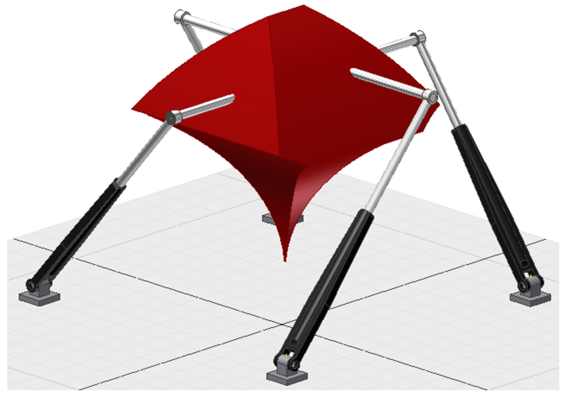
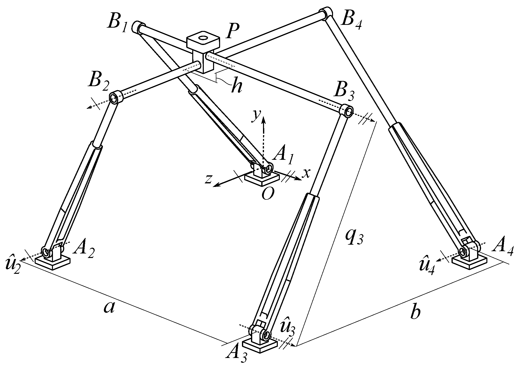
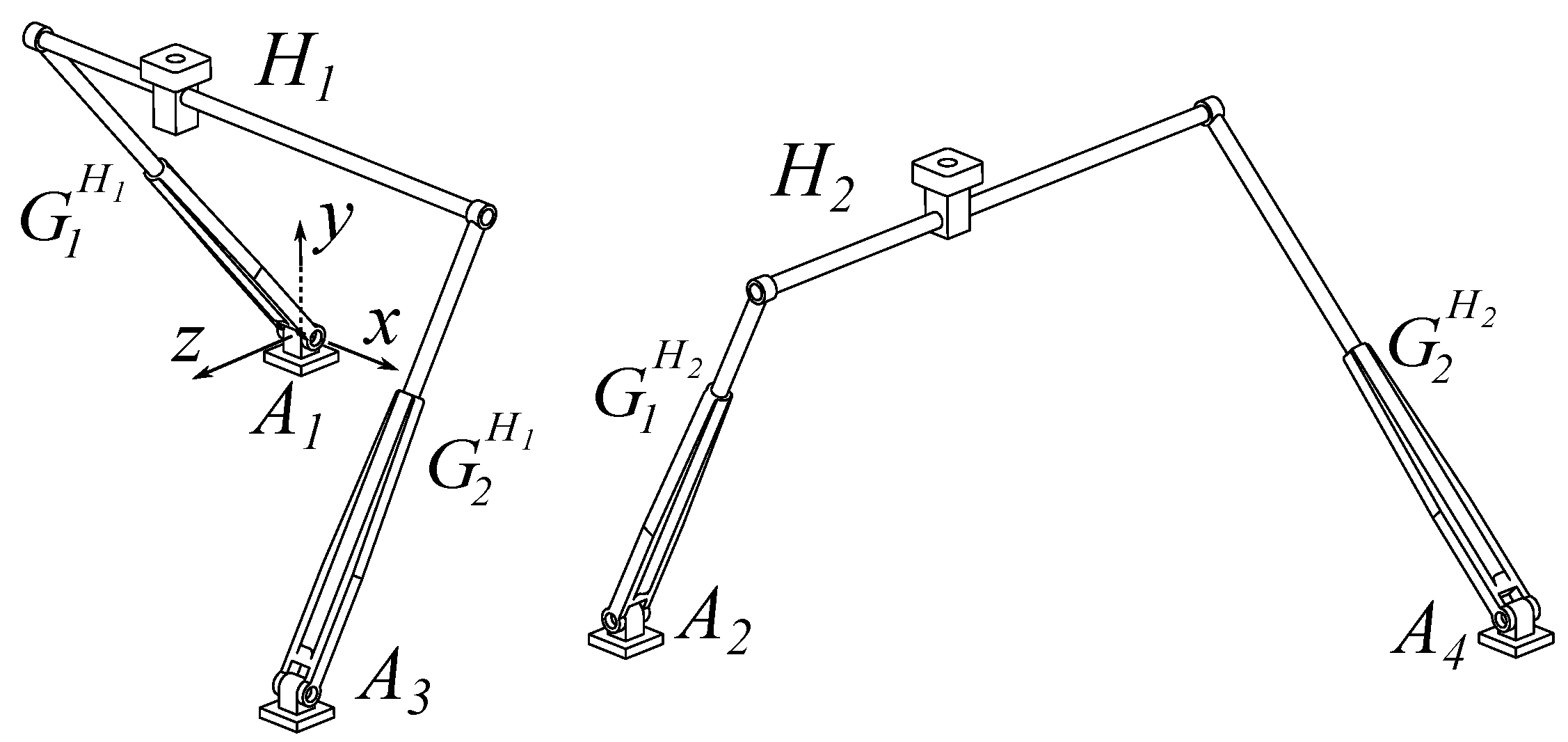
The proposed manipulator,
Figure 1, consists of four RPRP-type kinematic chains, three of which with the prismatic pair nearest to the base playing the role of active joint, and the fourth kinematic chain is completely passive. Unless otherwise specified, hereafter, the subscripts
refer to each of the three active kinematic chains, respectively.
The fixed platform of the manipulator is represented by the quadrilateral , with sides a and b. The fixed coordinate system is conveniently located at the point , its x- and z-axes lie on the plane defined by the quadrilateral, and the y-axis points upward. Points denotes the nominal position, which is located by vectors , of the first revolute joint of each kinematic chain. Similarly, denotes the nominal position, which is located by vectors , of the second revolute joint of each kinematic chain. Points and are separated in the same kinematic chain by a variable distance , which is actually a measure associated with the linear displacement of the i-th active prismatic joint. On the other hand, points and are connected by a rod, which is perpendicular to the rod that connects points and . Both rods are connected to the moving platform by prismatic joints, which are separated from each other by a vertical offset h. Finally, point , which is located by vector , is the interest point in the moving platform (end effector) and is conveniently located at the intersection point of the mobile platform with the top rod.
Note that the rotational axes, denoted by , of the revolute joints located at points and are parallel to the x-axis for , and parallel to the z-axis for . Moreover, in the same kinematic chain, the translation axis of the active prismatic joint is perpendicular to .
The workspace of the proposed robot is shown in
Figure 2, and it can be configured or optimized following the method presented in [
20].
To the best of the authors knowledge, the topology of the manipulator is original. The proposed mechanism can be used, for example, in 3D printing systems and rapid prototyping machines due its scheme of actuation and large workspace (
Figure 2).
3. Mobility Analysis
One of the most used ways to determine the mobility or degrees of freedom of a mechanism is through the well-known Chebychev–Grübler–Kutzback criterion. However, it has been demonstrated that this formulation is not applicable for all types of mechanisms because the calculation is complicated for architectures with multiple closed loops [
21]. Considering the above, Gogu [
22] proposes a method that is characterized by the decomposition of the mechanism in closed loops in order to analyze the mobility constraints. In this section, an adaptation of this method is applied over the proposed mechanism, where the mobility,
M, of the mechanism is defined by:
where
p is the number of joints,
is the number of degrees of relative motion permitted by the
i-th joint, and
r is the number of joint parameters that lose their independence after closing all the mechanism loops. The
r variable is defined as:
where
k is the number of closed loops in the mechanism,
is the connectivity of the
j-th closed loop
when it is disconnected from the mechanism,
corresponds to the total connectivity of the mechanism, and
is the total number of parameters that lose their independence in the closed loops. These variables are calculated as follows:
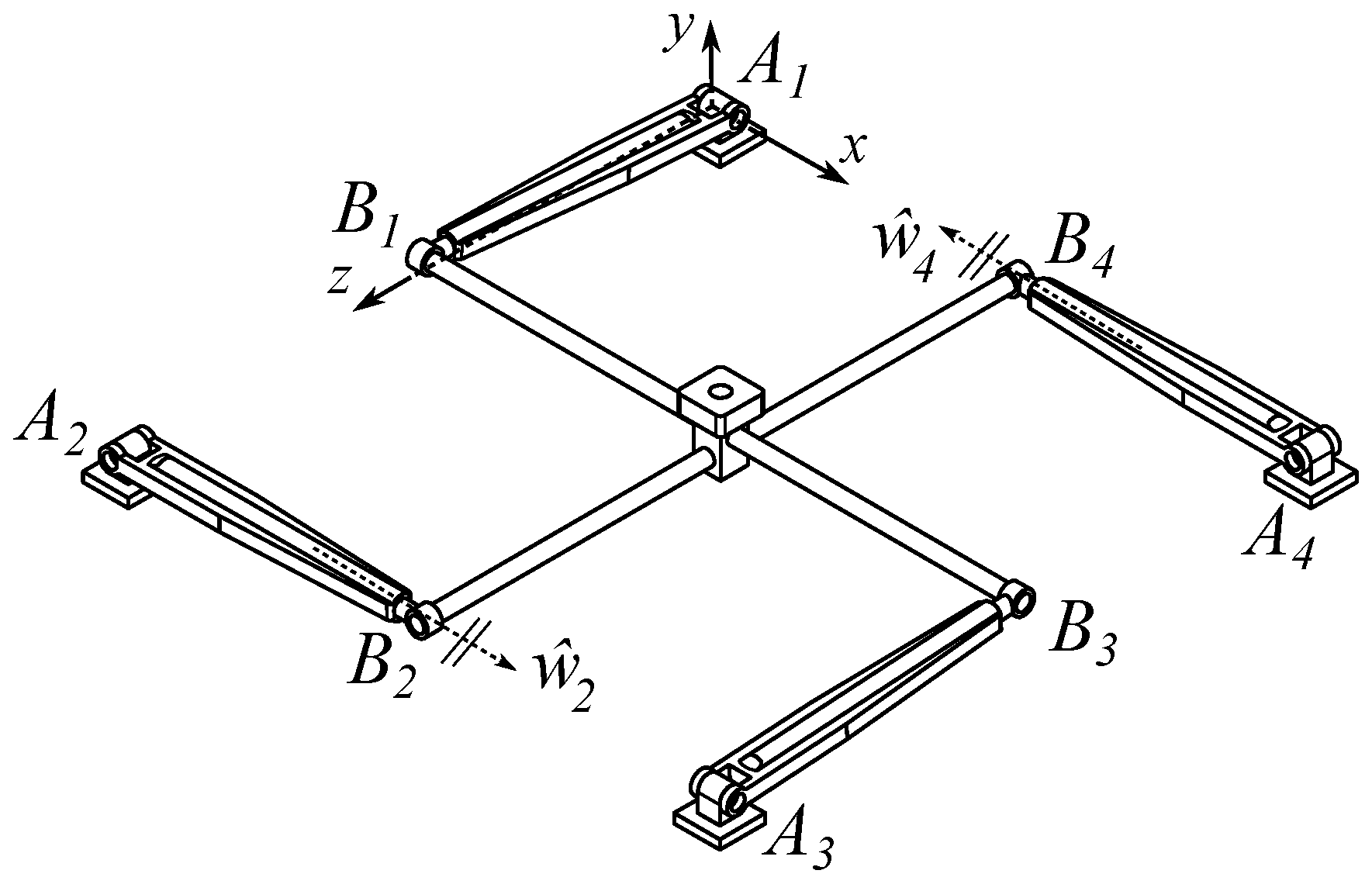
where
is the velocity vector associated with the interest point
P in the closed loop
(
Figure 3),
is the resultant velocity vector formed by the intersection of
, i.e.,
, and
is the number of parameters that lose their independence in the closed loop
. The variable
is defined by:
where
and
are, respectively, the connectivity of the limbs
and
in
, whereas
is the connectivity of the said loop. These variables are calculated as follows:
where
and
are the velocity vectors associated with
and
, and
is the resultant velocity vector formed by the intersection of
and
.
For the proposed mechanism, we can see that and . Furthermore, considering the fixed coordinate system located at the point , we can note that the velocity vector associated to the point P for each closed loop and are: and thus the connectivity of each loop is and . Considering the above, , and the connectivity of the mechanism is .
Disconnecting the limbs
and
from the mechanism and considering the fixed coordinate system, the velocity vector of each limb is:
and
, thus the connectivity of each limb is
. Considering the above,
and
and the connectivity of each closed loop is
.
From Equations (
5) and (
6), the number of parameters that lose their independence in each closed loops are
, and then,
. Considering this result, the number of joint parameters that lose their independence after closing all the mechanism loops is
Finally, considering that each joint has only one degree of relative motion, we obtain that the proposed manipulator has degrees of freedom.
4. Position Analysis
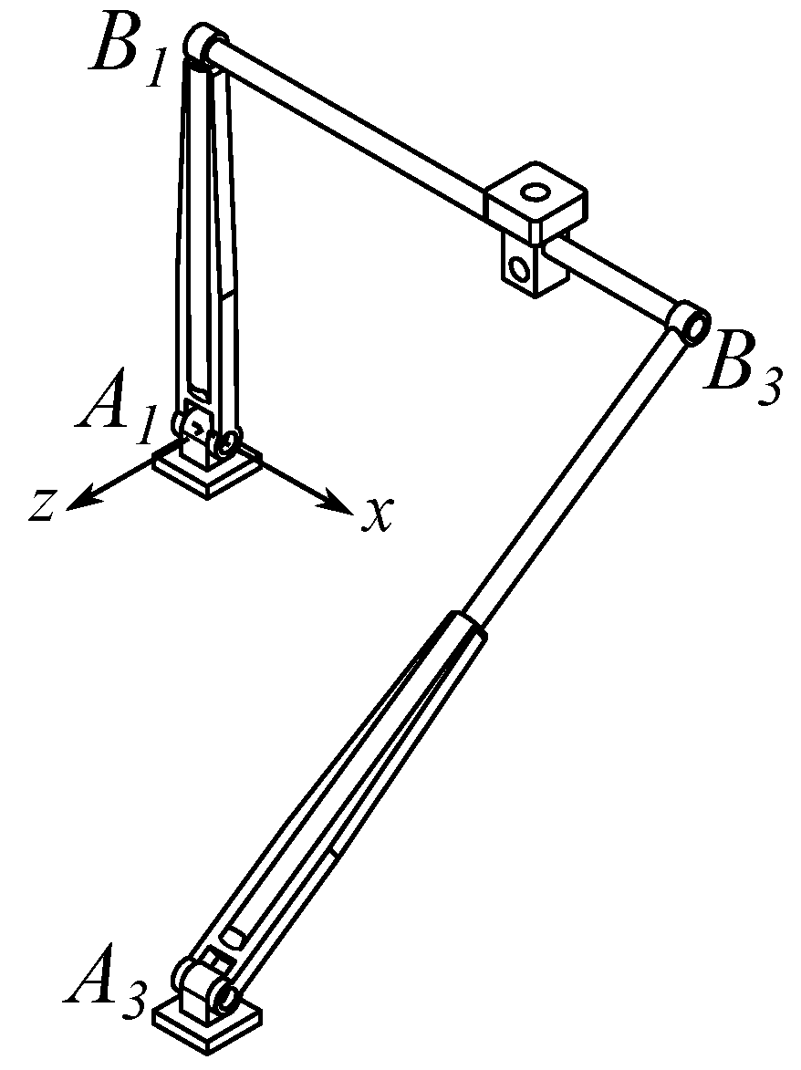
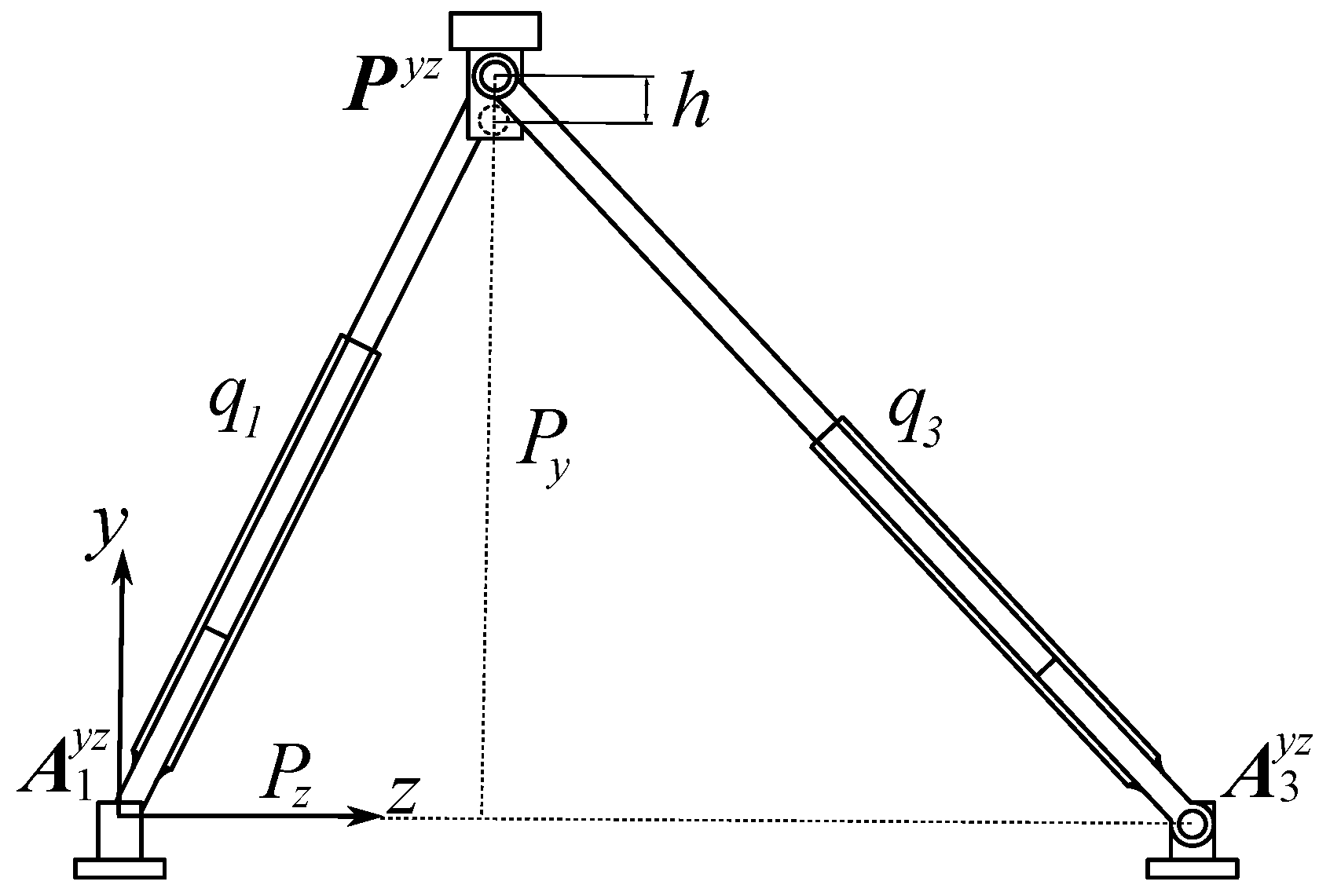
In this section, the displacement analysis of the proposed robot is solved. Since each of the limbs that form the manipulator have planar motion, it is convenient to study each of the closed loops as if they were two planar mechanisms. First, we consider the projection of the
loop onto the
-plane, as shown in
Figure 4. Note that the limb
is restricted between vectors
and
, which localizes the projections of the points
and
P onto the
plane, respectively. Its length,
, can be calculated as follows:
In the same way, for limb 3, we have:
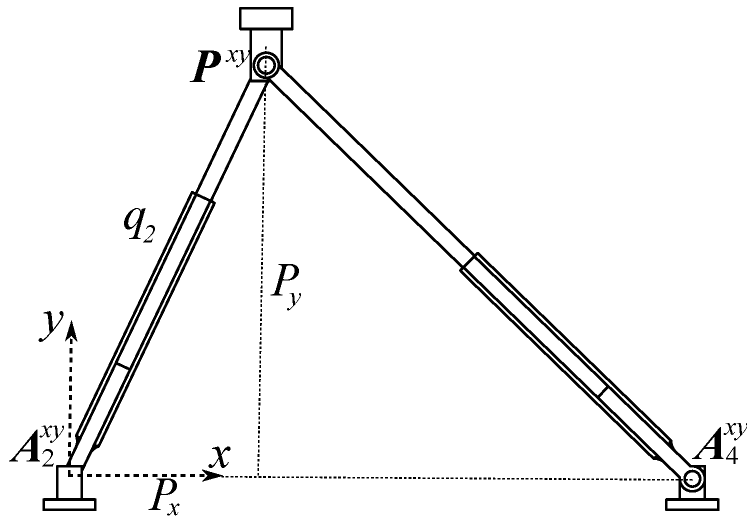
On the other hand, as presented in
Figure 5, from the projection of the closed loop
onto the
-plane it is possible to write:
The inverse position analysis, which is to determine the length of the active prismatic pairs to reach an arbitrary position of the moving platform, can be carried out by solving Equations (
9)–(
11), given the coordinates
of the moving platform.
The forward displacement analysis consist of finding the position of the moving platform if the length of the active prismatic pairs,
,
and
, are known. To this end, from the left side of
Figure 4, we can write the next expression:
meanwhile, from the right side, we have
By subtracting Equation (
13) from Equation (
12), it is possible to calculate
as follows:
Furthermore, from Equations (
12) and (
14), the coordinate
are determined following the equation
Finally, from Equations (
11) and (
15), the coordinate
may be calculated as follows:
It is easy to show that, solving Equations (
14)–(
16), it is possible to numerically obtain four possible positions of the point
P of the mobile platform. Of course, for practical applications
,
and
(see
Figure 1 and
Figure 2). Thus, only one solution is considered.
5. Velocity and Acceleration Analyses
In this section, the velocity and acceleration analyzes are solved by using the screw theory and the concept of reciprocity of screws.
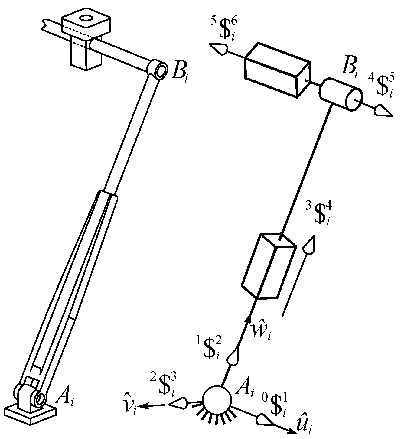
In order to complete the range of the Jacobian matrix, two
virtual revolute joints are introduced in each active limb of the robot, so they are modeled as
kinematic chain, as shown in
Figure 6, where the screws
and
associated with the virtual spherical pair are
fictitious. It is easy to show that this does not affect the mobility of the mechanism. Furthermore, the screws associated with the joints of the equivalent manipulator are:
where
is a unit vector along of the
i-th limb, such that
; meanwhile,
.
On the other hand, let
ω be the angular velocity vector of the moving platform as observed from the fixed platform. Furthermore, let
be the velocity vector of the center
O of the moving platform, where point
O plays the role of reference pole; in other words,
O is instantaneously coincident with a point of the reference coordinate system
. Then, the velocity state
, of the moving platform with respect to the base may be expressed through the
i-th limb as follows:
where
denotes the joint ratio velocity of the rigid body
as observed from the adjacent body
j, both belonging to limb
i. It is evident that
due to fact that the robot under study only can perform translational movements.
Furthermore, with reference to
Figure 6, please note that screw
is reciprocal to all the screws belonging to the
i-th limb except to
. Then, by applying the Klein form
between
and both sides of Equation (
17), we have
Casting into a matrix form, and for
, the input–output equation of velocity of the parallel robot results in
where
is the reduced Jacobian matrix of the manipulator; meanwhile,
is the generalized velocities vector, also called the first-order driver matrix of the parallel manipulator.
On the other hand, the inverse velocity analysis is to find the velocity ratios of manipulator
, a previous and necessary step in the acceleration analysis, for a given velocity state. Then, the joint velocities ratios can be determined as follows:
where
and
is the Jacobian matrix of the
i-th limb.
Equation (
19) is useful to find the singular configurations of the manipulator. Please note that, according to [
23], the robot is in a singular position when
, or, in other words, when vectors
,
and
are linearly dependents. This occurs, for example, when the limbs lie in the the same plane, or when two of them are parallel, etc. Some such configurations can be avoided with a proper selection of the dimensions of the robot. For example, singularity shown in
Figure 7 occurs when the limbs lie in the plane of the fixed platform, and this configuration can be avoided if in the same closed loop, the sum of the minimum linear displacement of the two active prismatic joints implicated is greater than the distance between the first revolute joint and the last one (this distance is measured parallel to the active prismatic joints). For instance, in the closed loop
, the following relation must be satisfied:
.
In the case of parallelism between limbs, it is important to mention that, because of the geometry of the robot, it is impossible for both limbs in the same closed loop to be parallel to each other. However, two limbs belonging to different closed loops could adopt a vertical configuration and be parallel. For example,
Figure 8 shows a case of this configuration for the closed loop
, specifically for the limb associates with linear displacement
, whose minimum value is obviously related to the maximum value of
. Considering the above, it is possible to define the following geometric relation:
. A similar relation should be established for the other limb and in general for the other closed loop in order to avoid this type of singular configuration. Furthermore, note that the mechanism does not have the so-called inverse kinematics singularities [
23], which represents an advantage over similar topologies.
On the other hand, following a similar procedure procedure as the one used in the velocity analysis, the input–output equation of acceleration can be written as follows:
where
is the acceleration of any point embedded to the moving platform, and
is given by
Moreover,
,
and
are the Lie screws, formed by Lie products
of its respective kinematic chain, and are given by
6. Inverse Dynamic Analysis
The driving forces of the translational parallel robot are calculated in this section by means of a combination of the screw theory and the principle of virtual work. This problem can be formulated as follows: given the inertial, gravitational and external wrenches, to determine the driving forces required to obtain the desired trajectory for the mobile platform.
According to the principle of D’Alembert [
24], the inertial wrench
acting on the
j-th body of the
i-th chain is given by:
where
is the mass of the body,
is the translational acceleration of the mass center, and
is the centroidal inertia tensor with respect to the global reference system. This matrix can be calculated by transforming the local inertia tensor,
, through rotation matrix
as:
We consider the gravitational wrench
, where
g is the acceleration of gravity and an external wrench
applied to the body
j at its center of mass. Then, the resultant wrench acting on body
j of the limb
i is
It is shown in [
25] that the power
produced by
that acts on the
j body of the
i-th chain with velocity state
, whose reference pole is its center of mass, can be determined by:
In order to apply the principle of virtual work, it is necessary to express
as a function of the generalized velocities
. From Equations (
19) and (
20):
where coefficients
n are elements of
:
From Equation (
26), the speed ratio of body
j respect to body
, belonging to chain
i, is expressed in terms of
as follows:
where the scalars
are the first order kinematic influence coefficients. Then, the velocity state of body
j belonging to the
i-th chain can be expressed as:
Then, grouping the terms in
, and taking the mass center of the body as representation pole, leads to:
where
and
are called
partial screws [
25,
26].
Thus, Equation (
25) can be rewritten as follows:
where
is the driving force associated to the generalized velocity
for
.
The principle of virtual work states that if a multi-body system is in equilibrium under the effect of external actions, and then the global work
produced by the external forces with any virtual velocity must be null [
24]. Taking into account the virtual velocities
, substituting Equation (
29) in Equation (
30), and rearranging terms, leads to
Since the generalized virtual velocities
are arbitrary, and
, it is necessary and sufficient that the coefficients of the virtual displacements
are zero:
Finally, from Equation (
32), the generalized forces
can be computed directly.
7. Numerical Example
To show the application of the method, in this section, a case study is reported. The parameters of the mechanism are given by
,
,
,
, and
, where all dimensions are expressed in mm. Furthermore, consider that the generalized coordinates are commanded to follow periodical functions given by
,
,
where
t is in the interval
. With this information, the first part of the numerical example requires calculation of all the solutions of the forward displacement analysis when
. Applying the methodology described in
Section 4, there are four real solutions for the position of the moving platform, and they are presented in
Table 2.
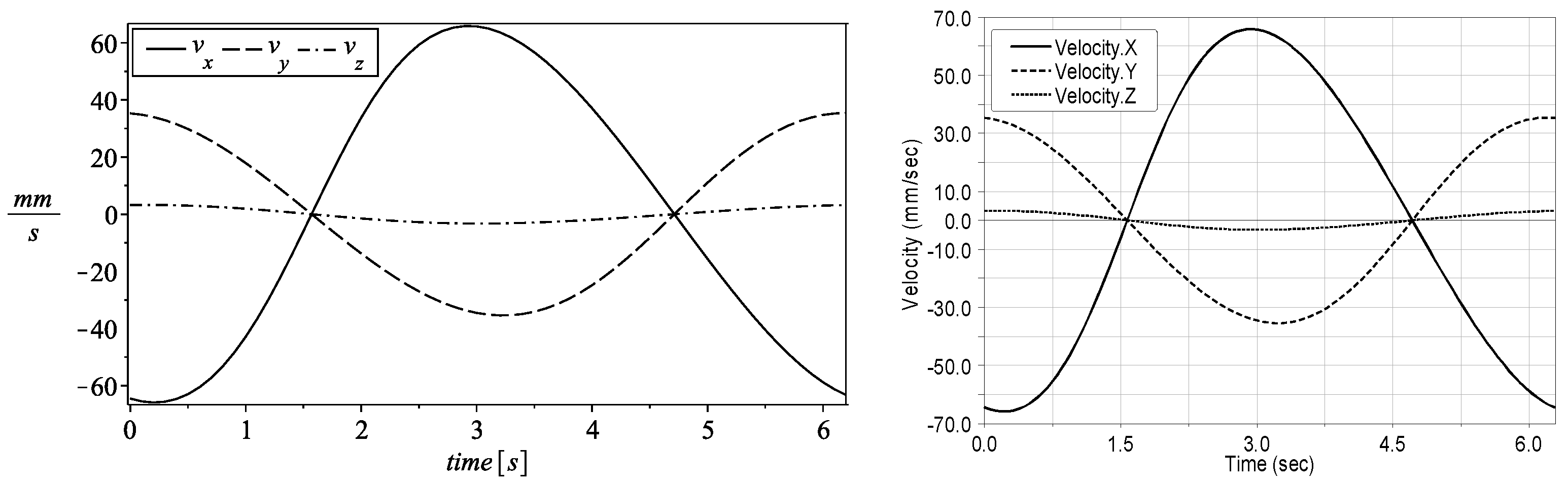
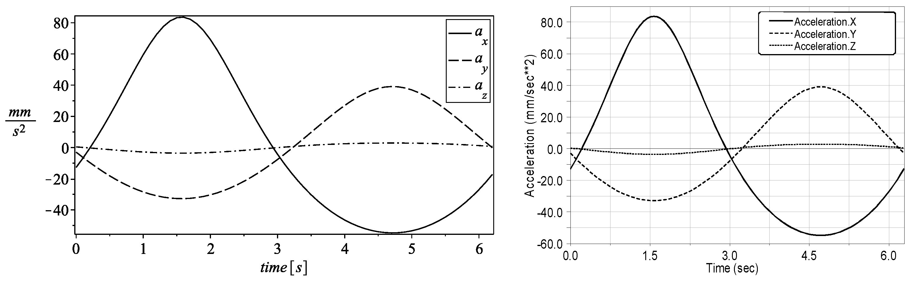
The second step in solving the example consists of computing the temporal behavior of the velocity and acceleration of point
P that belongs to the mobile platform. To this aim, the third solution of the forward displacement analysis is chosen as the home position of the robot at hand. The application of the method explained in
Section 4 and
Section 5 yields the results shown in
Figure 9 and
Figure 10, where they are compared with the numerical results obtained with the aid of commercially available software like ADAMS 2014.
Note that, according to
Figure 9 and
Figure 10, the numerical results obtained by using the theory of screws agree with those generated by means of a different approach such as the use of ADAMS.
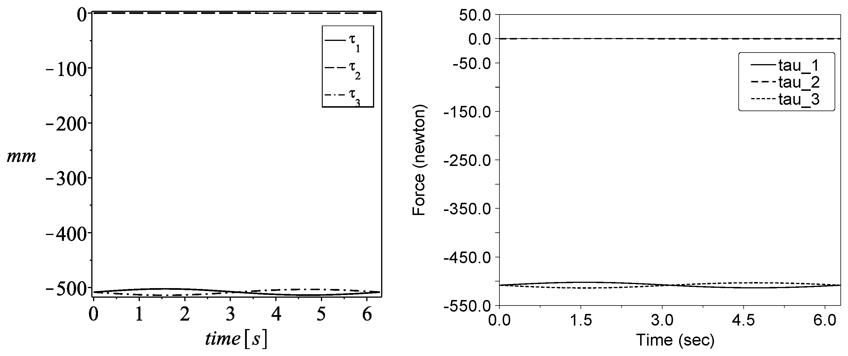
The last step of the numerical example consists of finding the driving forces that are required to execute the desired states of velocity and acceleration. In order to simplify the analysis, the following considerations are assumed: (a) body 5 is considered as part of body 6; and (b) body 1 is assumed as belonging to the cylinder, body 2. The inertial properties of the manipulator are depicted in
Table 3.
On the other hand, consider that the center of the moving platform is suffering a force of
N and a couple of 200 Nm where both vectors are normal to the plane of the moving platform along the entire trajectory imposed to the moving platform. With these data, and following the method presented in this work, the resulting temporal behavior of the three generalized forces are presented in
Figure 11.
8. Conclusions
A parallel robot with a novel architecture was presented in this paper. The mobility of this mechanism was studied by the well-known method of Gogu, concluding that it has three translational degrees of freedom. In addition, the equations of position analysis, which are notoriously simpler than other similar robots, were obtained and solved. The large work space, which is not discussed in this contribution, in addition to its scheme of actuation, allows the potential use of the manipulator in, for example, machining of soft materials, rapid prototyping tasks, 3D printing, and others. Furthermore, analyses of velocity and acceleration were solved by using the theory of screws and the Klein form. This analysis shows that it is possible to avoid some of the evident singularity configurations with an appropriate selection of the dimensions of the fixed platform. The generalized forces are determined by combining the principle of virtual work and the theory of screws through the Klein form of the Lie algebra of the Euclidean group . Finally, the results were validated by a simulation software of coinciding numerical simulations with the results predicted by the method presented.


