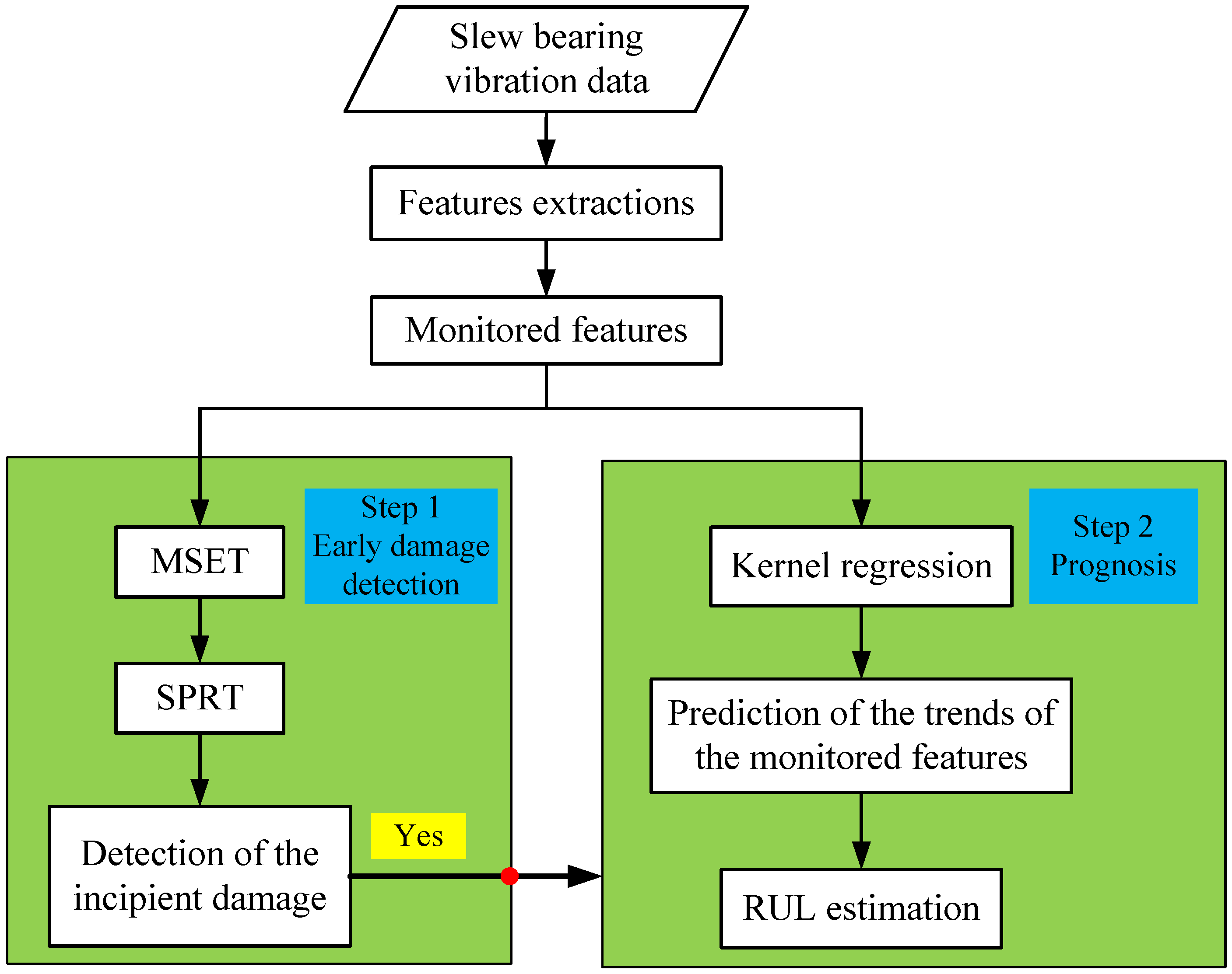
4.1. Step (1) Detection of the Incipient Slew Bearing Defect Using MSET and SPRT
Twelve features were extracted from four different methods [
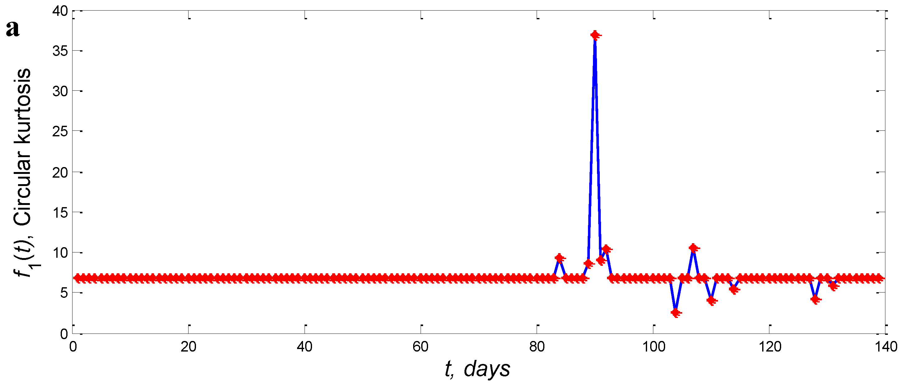
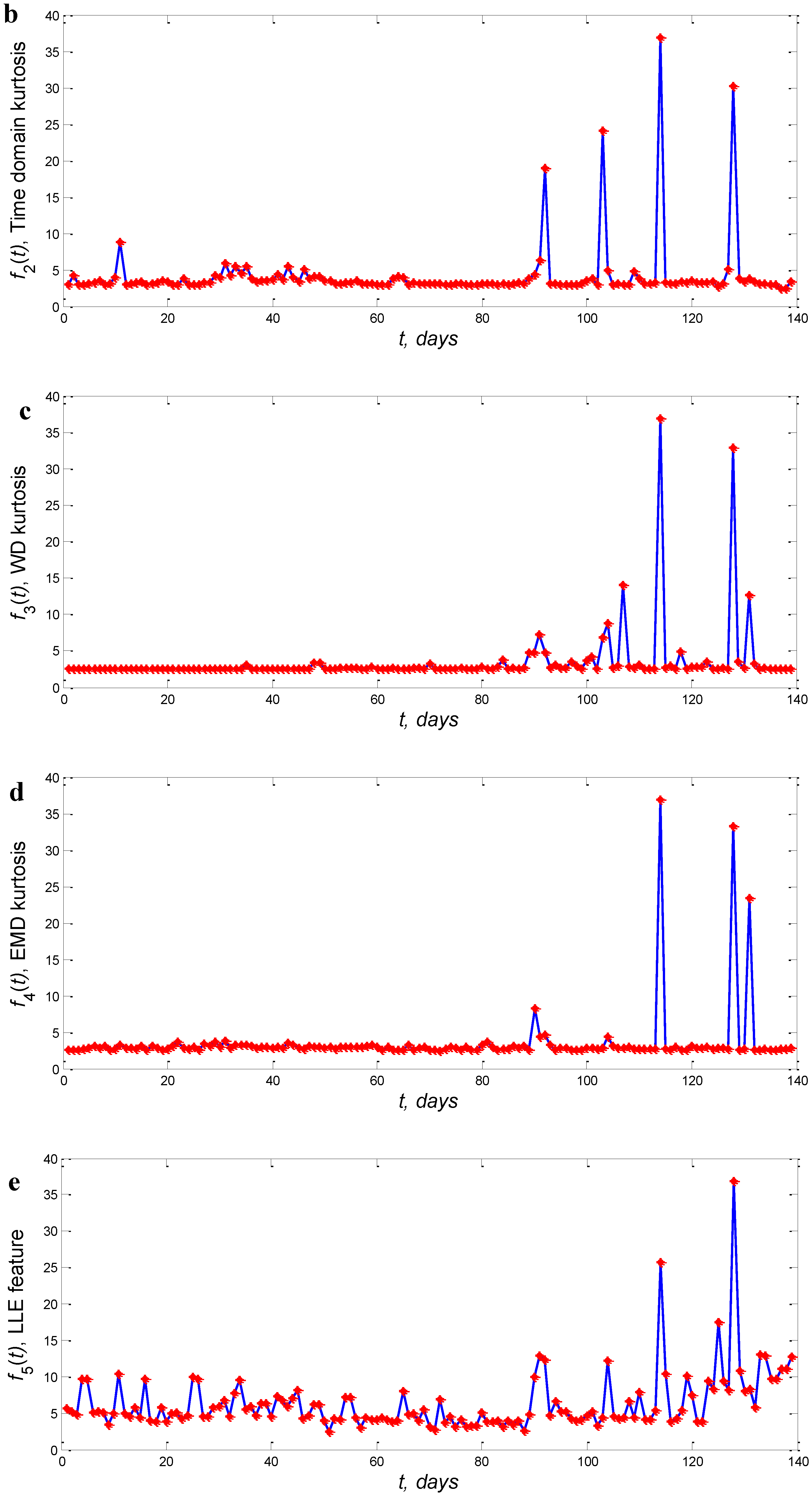
31]. Not all features were sensitive to the change of the bearing condition. Consequently, the method only uses five of the most sensitive features as the input to the MSET. The five features were (1) kurtosis extracted from accelerometer signal,
f1(
t); (2) kurtosis extracted from the piecewise aggregate approximation (PAA) combined with circular analysis,
f2(
t); (3) kurtosis extracted from the wavelet decomposition,
f3(
t); (4) kurtosis extracted from the EMD,
f4(
t); and (5) LLE feature obtained from the largest Lyapunov exponent algorithm,
f5(
t) [
32]. The five features were extracted over the 139 days test period. The plot of the aforementioned features has been shown in
Figure 2. These features are used to establish data matrix
P. Thus, the dimension of data matrix
P in Equation (1) is 5 by 139, where 5 is the number of features and 139 is the number of days.
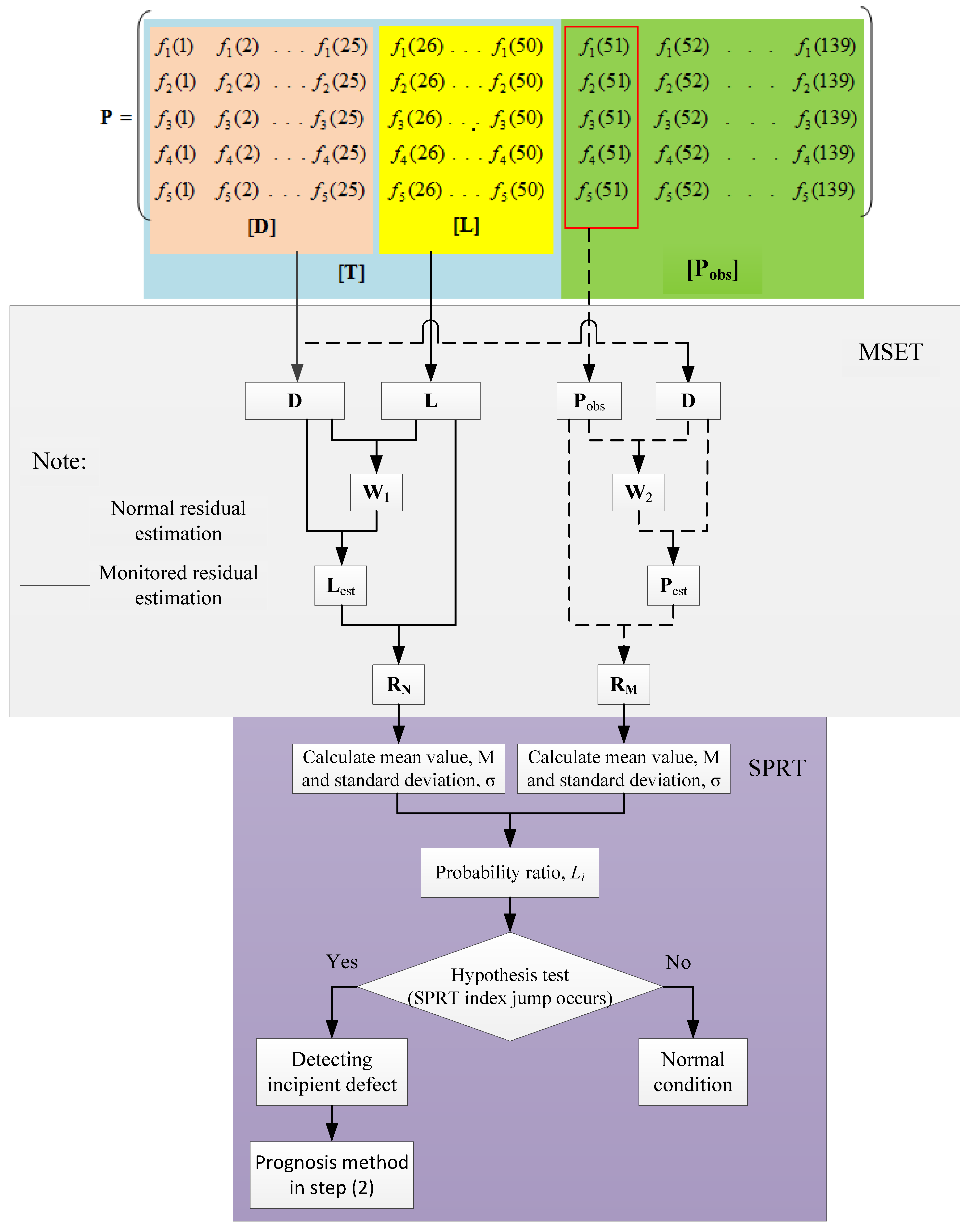
To detect the incipient slew bearing defect (Step 1), the MSET algorithm calculates the normal residual matrix (
RN) and the residual matrix of monitored state (
RM) (see
Figure 3). In Step (1), the following inputs are required: training matrix
T, memory matrix
D, remaining training matrix
L and observation matrix
Pobs. In this paper,
T of 50 days was used. In the computation, the sizes of matrices,
D and
L have to be half of
T i.e., 25 days each. The reason why 50 days was used is because coal dust was not injected until day 58. In other words, during the first 50 days, the vibration signal had been acquired when the condition of the bearing was still normal. In practice, matrix
Pobs is obtained from daily observation or measurement. The number of measurement days from normal to failure has been set as 139 days.
Pobs is the matrix from day 51 to day 139.
After
D and
L have been determined, the weight of normal state vector (
w1) is then calculated using Equation (3) by employing the Euclidean distance as the non-linear operator. Vector
w1 represents the weight of normal data points in the training data.
w1 is used to calculate the normal estimate matrix (
Lest) using Equation (5). And the normal residual matrix (
RN) is estimated by taking the difference between
Lest and
L, as shown in Equation (7). It should be noted that prior to the calculation of the statistical properties, matrix
RN is normalized with a zero mean. This is necessary for the next process in the SPRT method because under normal bearing conditions the mean value of the normal residual matrix (
RN) is expected to be ≈0. The result of normalized matrix (
RN) is presented in
Table 4. A similar procedure is also employed to obtain the residual matrix of monitored state (
RM). Equation (4) is used to calculate the weight of monitored state vector (
w2), Equation (6) is then used to calculate the estimate matrix of monitored state (
Lest) and Equation (8) to calculate the residual matrix of monitored state (
RM). Matrix
RM is then normalized within a range between maximum value and minimum value of the normalized normal residual matrix (
RN). The calculation of
RN and
RM is the final step of MSET. Both results are then fed into the SPRT.
In SPRT, statistical characteristics such as mean value, standard deviation and the range between maximum and minimum values are calculated from each column of normalized matrix
RN. These statistical properties belong to the normal condition of the bearing are used as the reference normal data. These properties also form the set of hypotheses in SPRT. For the monitored state, prior to the calculation of the mean value and the standard deviation, the matrix (
RM) is normalized within the range between maximum and minimum value of the normal state. The mean and standard deviation values of the normal state (up to days 25) are presented in
Table 5 and
Table 6, respectively. The detection of the incipient slew bearing defects is obtained by comparing the statistical characteristics, the mean value and the standard deviation) of the monitored state to the statistical characteristics of the normal state.
This comparison is repeated to the 51 to 139 columns of the
Pobs matrix. If the mean value or the standard deviation in each day lies outside the range of the reference mean values (
Table 5) or standard deviation values (
Table 6), incipient defect is considered to have occurred. This step is part of the SPRT procedure. To make a comparison, the list of hypotheses must be determined first including the normal condition (H
0) represented by mean value = M
normal and the standard deviation = σ
normal. Alternatives hypotheses H
1 to H
4 indicate the abnormal conditions. The set of hypotheses is given in
Table 1.
To measure the comparison mathematically, the ratio of the probability of alternative hypotheses (H
1 to H
4) and the probability of the null hypothesis (H
0) is calculated, Equation (10). Once probability ratio
Li is obtained, the SPRT index can be calculated by taking the natural logarithm of probability ratio
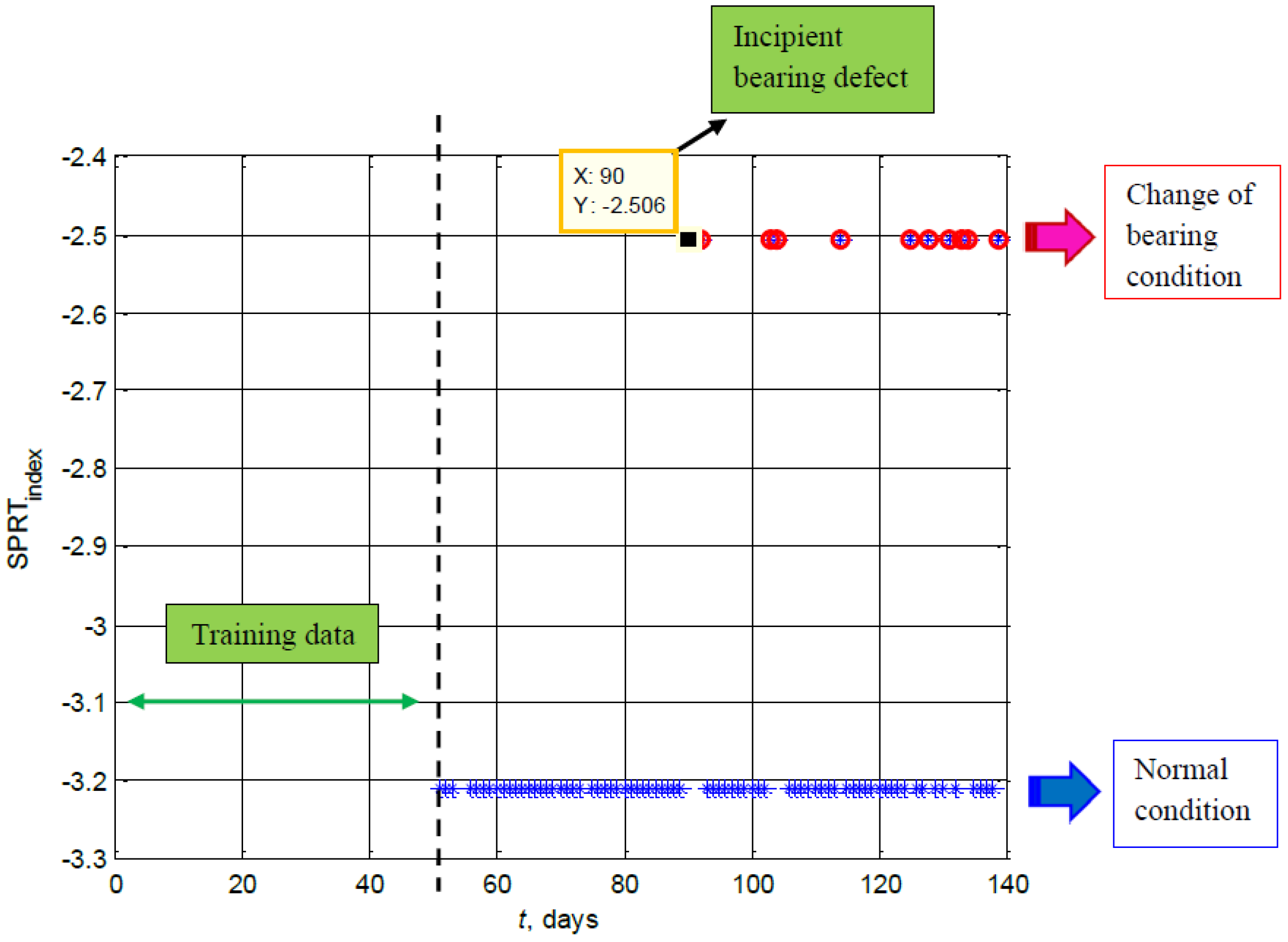
Li. The result of Step (1) is presented in
Figure 8. It can be seen from the monitored data of day 51 to day 89 that the bearing is still in normal condition. The impending deterioration of the bearing is identified on day 90. Note that the impending deterioration is needed in Step (2) to predict the future state and to estimate the RUL estimation. A sample calculation of
Li for a day (day 51 and day 90) is presented in
Table 7. When the condition of the bearing is still normal, the probability of statistical properties {
Si} that fall within the hypotheses H (
p({
Si}/H)) is much lower than the probability of statistical properties {
Si} of the null hypothesis H
0 (
p({
Si}/H
0)). To illustrate the normal condition (i.e., day 50), the natural logarithmic of
Li is given in
Table 7 and shown in
Figure 8. On the contrary, on day 90 the condition of the bearing started to deteriorate, the probability of statistical properties {
Si} that fall within the hypotheses H (
p({
Si}/H)) will increase and the probability of statistical properties {
Si} that fall in the null hypothesis H
0 (
p({
Si}/H
0)) will decrease, the natural logarithmic is then given in
Table 7 and shown in
Figure 8.
4.2. Step (2) Prediction of the Future State of Selected Features Using Kernel Regression
Features extracted from slew bearing vibration signals have different characteristic to those extracted from accelerometers signals of typical rolling element bearings. In typical rolling element bearings, when the bearing condition deteriorates, the features values increase gradually. In slew bearings, the changes of the slew bearing condition can be detected from a sharp increase of feature value. However, this value does not increase steadily as it does in typical high speeds roller bearings. The extracted features of the slew bearing signal usually revert to the normal level and rise again as the condition has deteriorated significantly. This condition is referred as ‘self-healing’ characteristic [
41]. This is one of the difficulties in defect prediction especially for data-driven prognosis methods [
42,
43,
44]. In this paper, the problem has been overcome using kernel regression. Prior to the use of kernel regression, all features have to be evaluated. Caesarendra et al. [
32] presented four evaluation criteria to track the progressive bearing defect. In the present study, another evaluation criterion based on exponential function is proposed. It is well known that as bearing deteriorates, certain features will increase exponentially. Hence, an evaluation criterion (
E) obtained from the coefficient of the exponential curve fitting of the feature being evaluated is used as illustrated below. Suppose
f(
t) is the monitored evaluation function.
where
a and
E are the curve fitting exponential coefficients, and
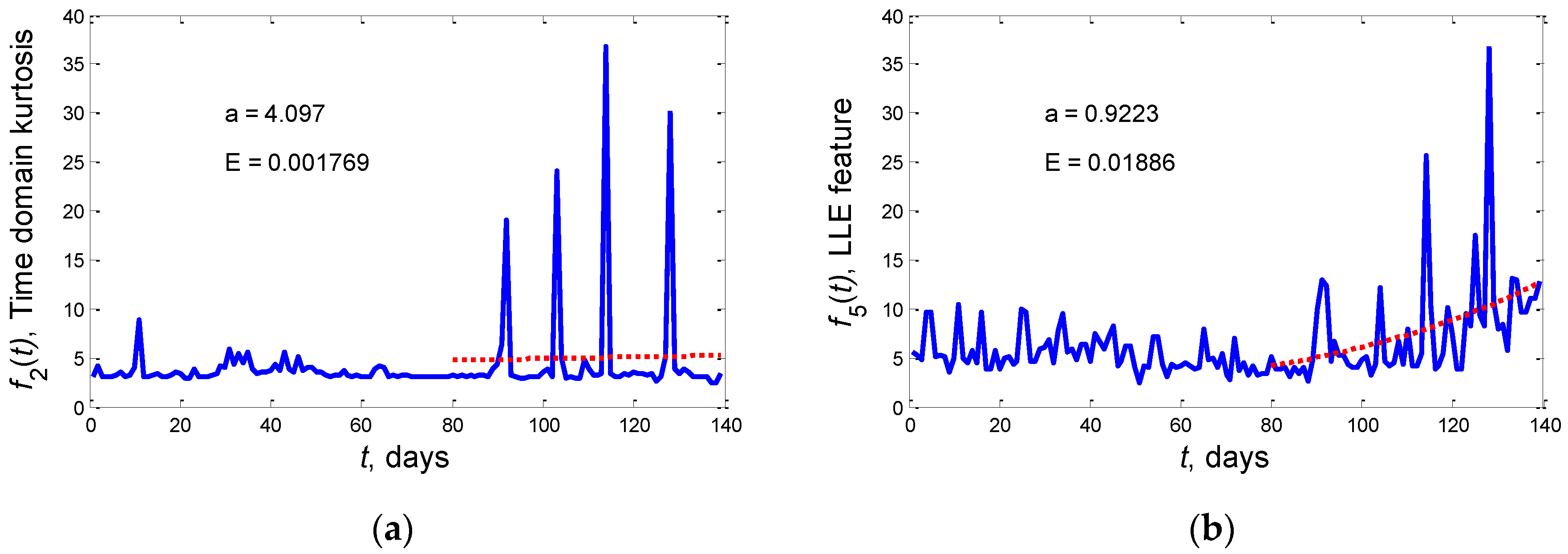
t is the measurement days. The calculation of
E for the time-domain kurtosis feature and the LLE feature is presented in
Figure 9. The two figures show clearly that the LLE feature shows a greater exponential increasing trend than the time-domain kurtosis feature. The dotted line in
Figure 9a,b is the exponential curve fitted from day 80 to day 139.
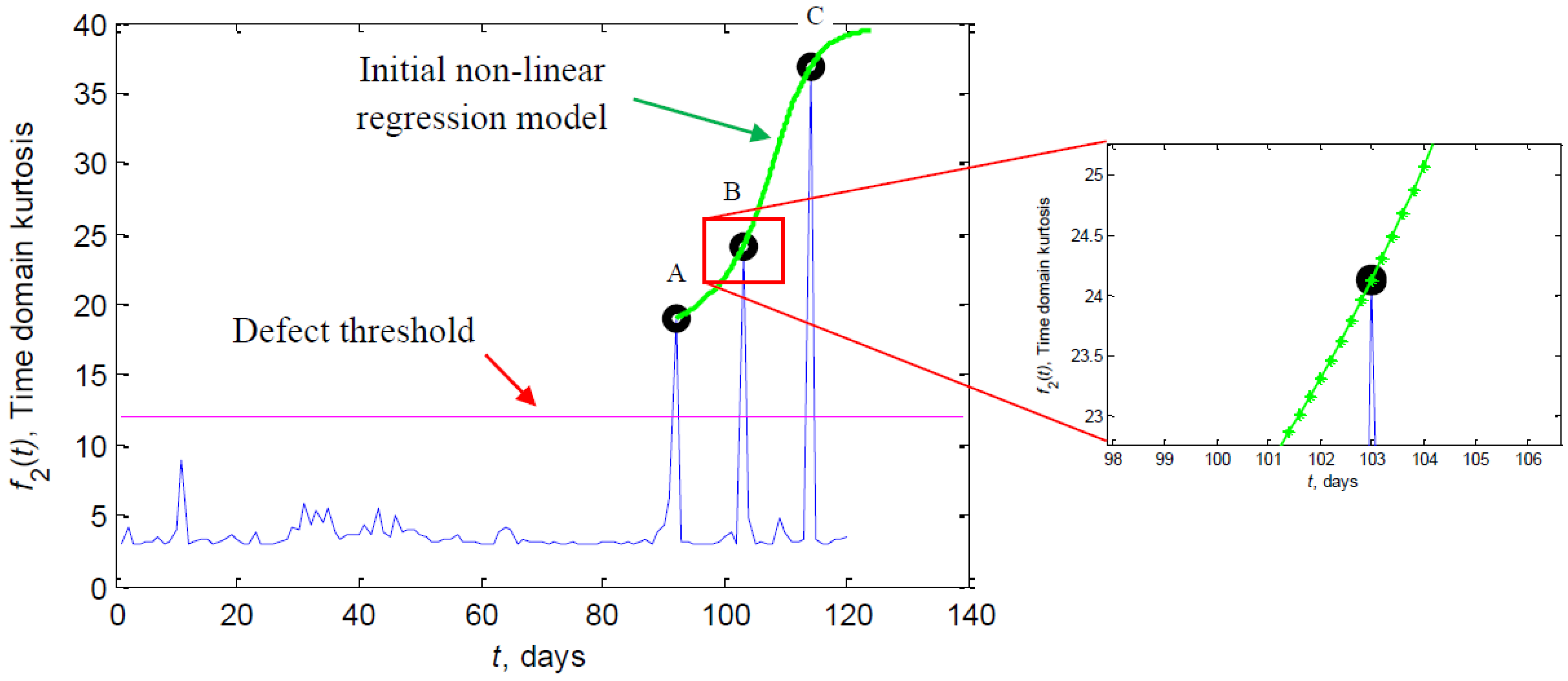
In Step (2), kernel regression is employed to predict the future bearing condition and to estimate the RUL of the slew bearing. This prediction starts when there is warning of impending deterioration of the bearing condition. The basic kernel regression algorithm is improved by adding a k-step-ahead subroutine. At each k-step, non-linear regression model and posterior (predicted) point is estimated and updated. The purpose of this process is to estimate a one-step-ahead prediction of the kernel regression model based on past non-linear data points.
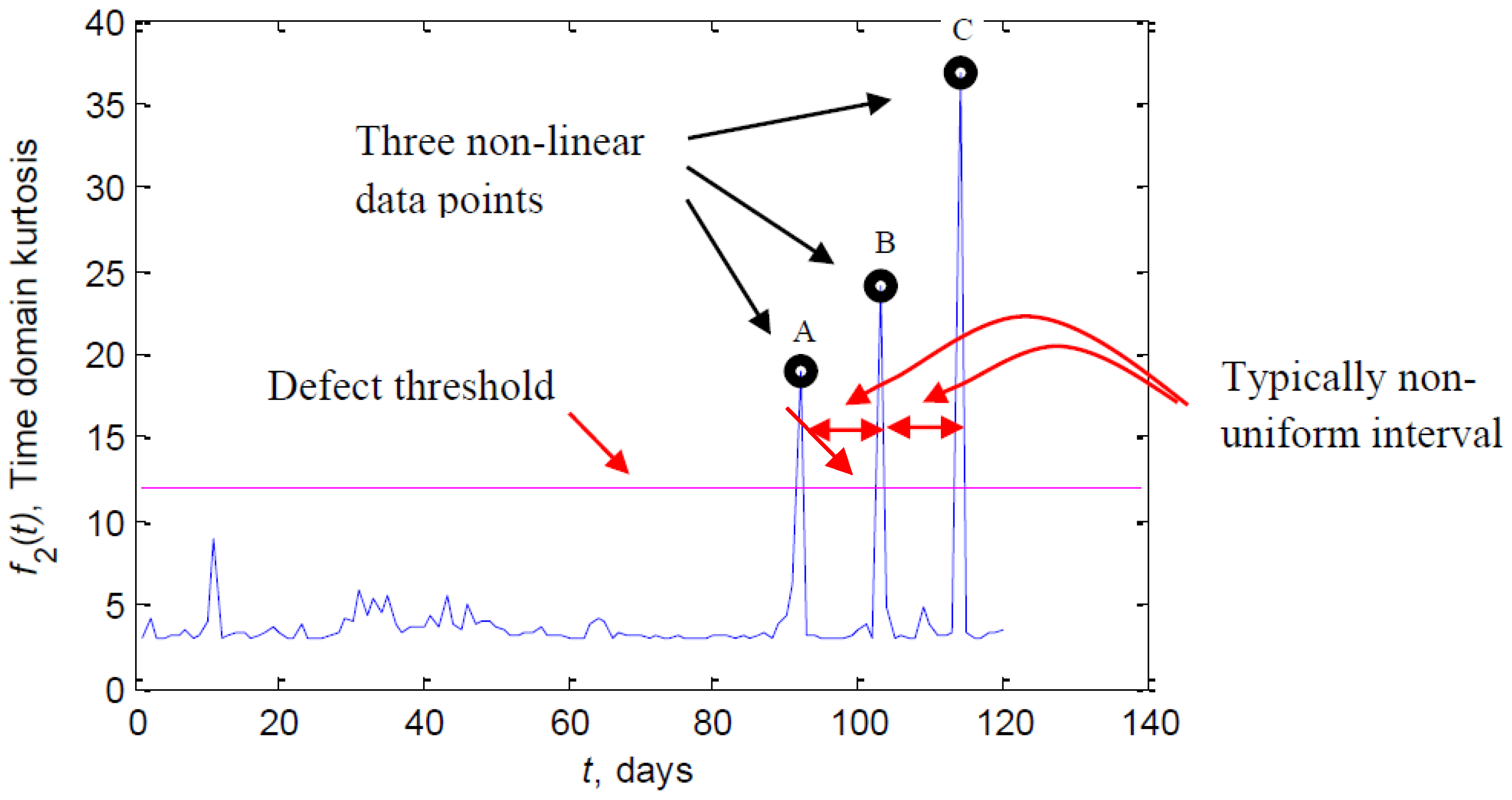
Kernel regression is an effective method to build a model from non-linear data. The process is done by taking the highest data point of the current kernel regression model and then using it as the next data point (e.g., predict the 4th data point if the initial model is built from three data points). The new data point is then used to build a new kernel regression model and estimate the next data point. The process is repeated until the specified k-step-ahead prediction is reached. To illustrate the process, a time domain kurtosis feature is used as the monitored parameter being predicted.
Kurtosis is selected as an input of kernel regression because it has a certain value for normal bearing condition and the kurtosis value for defect condition. This is necessary for the detection of incipient defect in Step (1), which is set with the predetermined warning threshold and for prediction in Step (2), which is set with the damage bearing threshold. The kurtosis value for normal bearing signals is approximately 3 [
40]. The increase of this value indicates that the bearing condition has changed. Some research mentioned that the kurtosis value will reach about 50 when high impact occur [
45]. Aye [
46] studied the kurtosis of normal and faulty tapered bearings running at speed between 409 RPM and 1200 RPM. It has been found that the kurtosis value for normal bearings is 2.89. Surprisingly, the kurtosis value for faulty bearings with 409 RPM increases significantly to about 30.26 and for 1200 RPM drops to 1.23. The same author [
46] demonstrated that the kurtosis value of bearing damage with low rotational speed (low RPM) can be much higher than the normal value. Guo et al. [
47] presented a method for recovering the bearing signal from large noisy signal using a hybrid method based on spectral kurtosis and ensemble EMD. It was found that the kurtosis value of each bearing fault condition was recovered and identified more easily. For instance, the kurtosis value of a bearing with an inner race defect and a ball defect is 18.35 and 41.20, respectively.
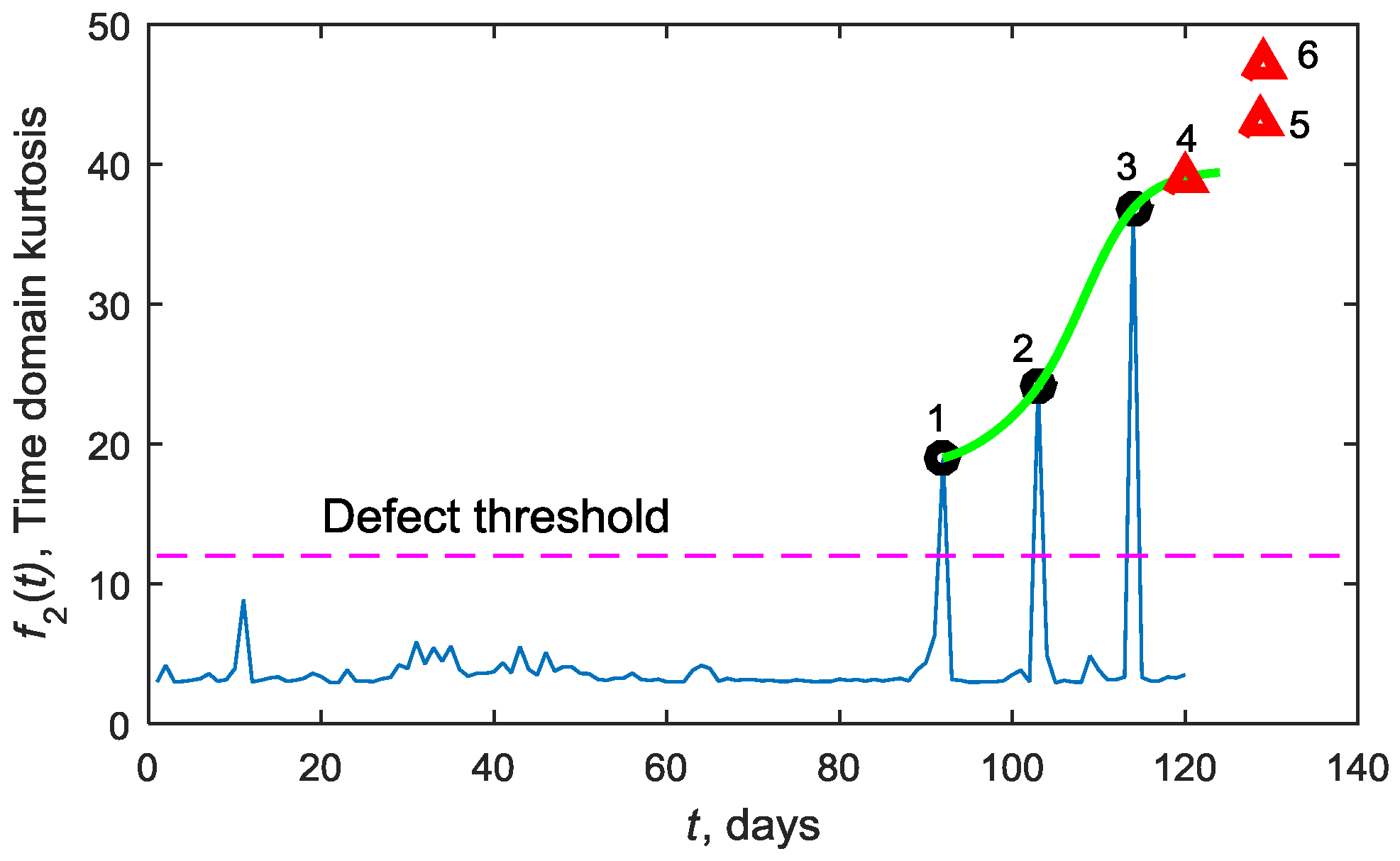
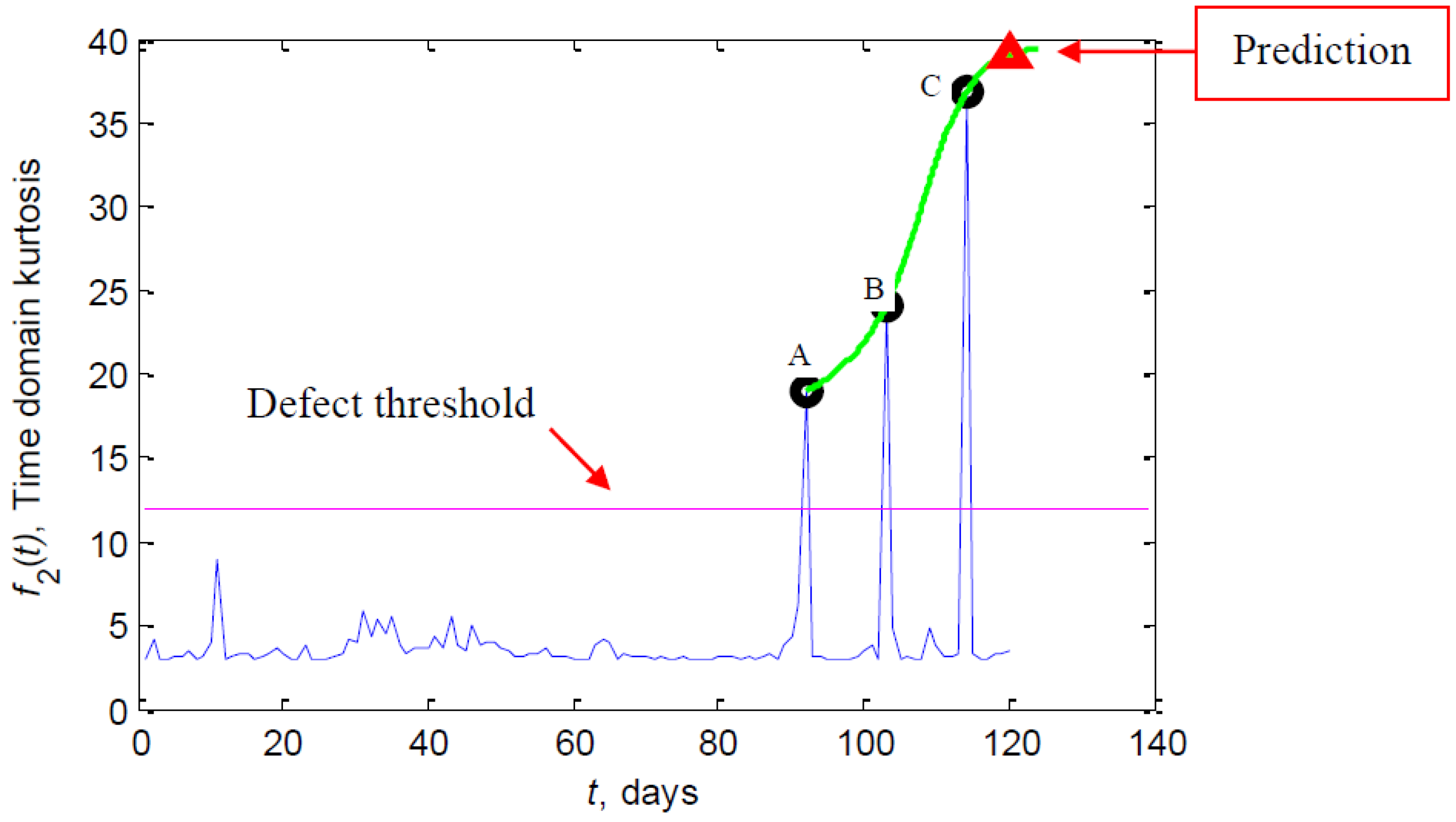
Supposed 3 points are available denoted as point 1, 2, and 3 as shown in
Figure 10. Firstly, the method predict one-step-ahead of degradation parameter denoted as point 4 (red triangle) based on 3 points i.e., point 1, 2 and 3. Secondly, to predict next degradation parameter denoted as point 5, the method used point 2, 3 and 4. Thirdly, to predict point 6 the method used point 3, 4 and 5. According to the
Figure 10, the plotted curve shows an increasing trend, it is due to the first 3 points used has an increasing trend. Thus for next prediction the method employed both actual value and predicted value to predict the next degradation parameter. In practice, when the kurtosis value is acquired from online condition monitoring, the points can be replaced by actual kurtosis value. The method will use 3 updated kurtosis values to do one-step-ahead prediction.
Setting a threshold level are depends on the different situations and types of bearings. The information can be obtained from the maintenance engineer or past condition monitoring (CM) data with has similar type of bearing and load condition. As has been done in past works [
45,
46,
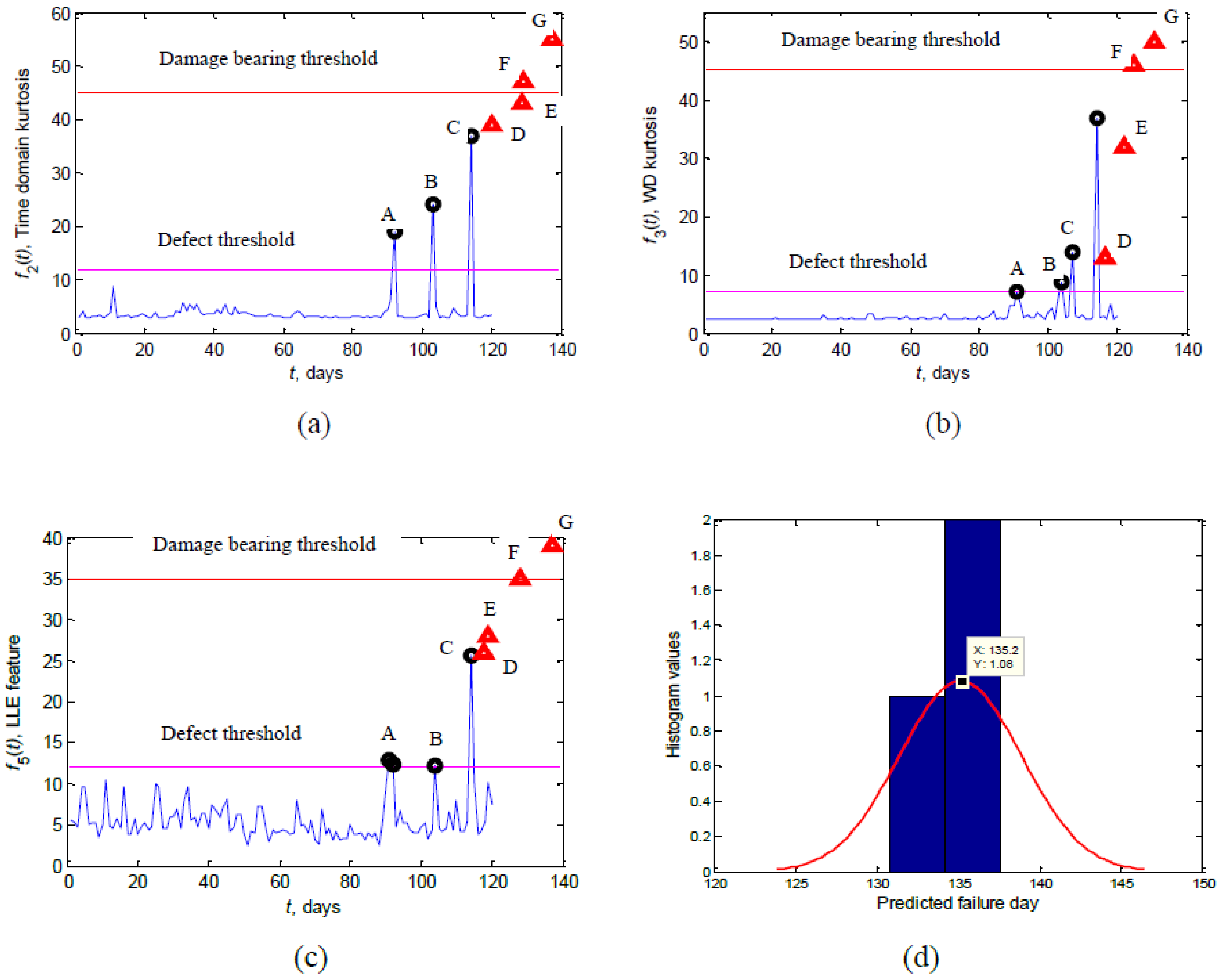
47], we have set the threshold kurtosis value of 45 for the time-domain kurtosis and the WD feature, while the threshold for the LLE feature is set at 35. The proposed kernel regression method was applied up to 120 days, as by day 120 the kurtosis value has exceeded 4 times the normal value and three data points greater than the alarm threshold level have been detected. It should be noted that three data points is the minimum requirement in the initial kernel regression model. Note that the levels of the three selected features up to day 120 are still below the bearing damage threshold of 45. The predictions of the kernel regression of the three features mentioned above are presented in
Figure 11a–c. The four step-ahead of kernel regression are used (
k = 4) and thus the 4 step-ahead predicted data points are shown with ‘Δ’ symbol, while ‘o’ represents the actual value. It can be seen that the predicted future values increases. When the data point exceeds the damage threshold level, the last predicted day is noted and used to estimate the histogram of final failure. Once the histogram of final failure is obtained, the RUL can be easily estimated by taking the difference between the predicted final failure time and the last measurement day (the last measurement day is 120).
Based on this analysis, the predicted failure day of the bearing is shown to be dependent on the features and summarized in
Table 8. Detail information of the three non-linear data used to build the initial model and the predicted data point of the modified kernel regression method for each feature is shown in
Table 9,
Table 10 and
Table 11 (point A–D). It is shown in
Figure 11b,c is the WD kurtosis feature and LLE feature, respectively. For WD kurtosis feature the spacing is different (day 104th − day 91th = 13 days and day 107th − day 104th = 3 days). The LLE Feature also has different spacing (day 104th − day 92th = 12 days and day 114th − day 104th = 10 days). Points D–G are the predicted features values. These points are estimated based on the 4-step-ahead prediction of the kernel regression. According to the results in
Table 9,
Table 10 and
Table 11, the
y-axis values of the fourth predicted points exceed the bearing damage threshold. The day of each fourth predicted point (point G) is noted as the final failure of the slew bearing. Three predicted days (point G) are then inputted to the histogram. The result of this is presented in
Figure 11d. It should be noted that with more features used, the more accurate the distribution fit of the histogram will be. It can be seen from
Figure 11d that the predicted final failure is day 135. Further, the RUL of the bearing can be estimated by taking the difference between the predicted failure day and the last measurement day i.e., 135 − 120 = 15 day. The final failure histogram was calculated using a common MATLAB function ‘histfit’. The probability curve is plotted based on the predicted final failure from three methods: (a) time-domain kurtosis at 137.6 day; (b) WD kurtosis at 130.8 day; and (c) LLE feature at 137 day.
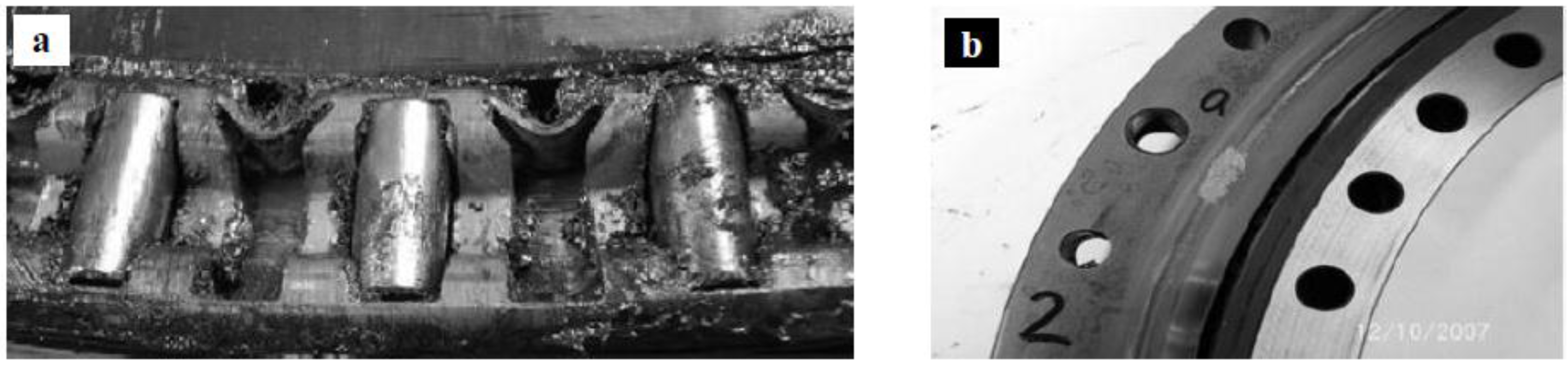
During the slew bearing lab experiment, complete failure is unpredictable. When a burst vibration signal on day 141 was detected, the test-rig had to be shut down. To inspect the damage and verify the result of the proposed prognosis method, the slew bearing was dismantled and inspected. Some of the defective rollers and outer race can be clearly seen in
Figure 12. The actual final failure day of lab slew bearing is considered one day before the severe burst vibration signal i.e., day 140. The accuracy of prediction is estimated as follows:
where
ta is actual final failure day and
tp is predicted failure day.


