Article

A Minimal-Sensing Framework for Monitoring Multistage Manufacturing Processes Using Product Quality Measurements †

NSF I/UCRC for Intelligent Maintenance Systems (IMS), University of Cincinnati, Cincinnati, OH 45221, USA
*
Author to whom correspondence should be addressed.
This paper is an extended version of the conference paper: Ardakani, H.D., Phillips, B., Bagheri, B., Lee, J. “A New Scheme for Monitoring and Diagnosis of Multistage Manufacturing Processes Using Product Quality Measurements.” The Annual Conference of the Prognostics and Health Management Society (October 2015).
Machines 2018, 6(1), 1; https://doi.org/10.3390/machines6010001
Submission received: 22 December 2017 / Revised: 2 January 2018 / Accepted: 4 January 2018 / Published: 5 January 2018
(This article belongs to the Special Issue Machinery Condition Monitoring and Industrial Analytics)

Abstract

:
For implementing data analytic tools in real-world applications, researchers face major challenges such as the complexity of machines or processes, their dynamic operating regimes and the limitations on the availability, sufficiency and quality of the data measured by sensors. The limits on using sensors are often related to the costs associated with them and the inaccessibility of critical locations within machines or processes. Manufacturing processes, as a large group of applications in which data analytics can bring significant value to, are the focus of this study. As the cost of instrumenting the machines in a manufacturing process is significant, an alternative solution which relies solely on product quality measurements is greatly desirable in the manufacturing industry. In this paper, a minimal-sensing framework for machine anomaly detection in multistage manufacturing processes based on product quality measurements is introduced. This framework, which relies on product quality data along with products’ manufacturing routes, allows the detection of variations in the quality of the products and is able to pinpoint the machine which is the cause of anomaly. A moving window is applied to the data, and a statistical metric is extracted by comparing the performance of a machine to its peers. This approach is expanded to work for multistage processes. The proposed method is validated using a dataset from a real-world manufacturing process and additional simulated datasets. Moreover, an alternative approach based on Bayesian Networks is provided and the performance of the two proposed methods is evaluated from an industrial implementation perspective. The results showed that the proposed similarity-based approach was able to successfully identify the root cause of the quality variations and pinpoint the machine that adversely impacted the product quality.

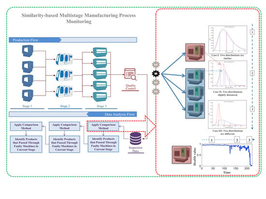
Graphical Abstract

1. Introduction

The complexity of manufacturing processes presents a major challenge for understanding the variations in the process and minimizing them to reach consistent quality of the products. Recent advancements in technology, however, provides significant opportunities for manufacturers to create value by implementing Internet of Things (IoT) and big data analytic tools and move towards smart enterprises with increased efficiency and profitability. From a manufacturing perspective, such trend is driving the manufacturers to improve their product quality and productivity by deploying advanced and reliable manufacturing process monitoring systems. A comprehensive review of the recent advances in modern manufacturing with regard to intelligent maintenance, scheduling and control is provided in [1]. For example, in the automobile body assembly process, optical coordinate measurement systems have facilitated the full measurement of dimensions for ensuring the quality of the final products [2,3]. As a result, an increasing number of researchers have focused on the development of data-driven monitoring systems for manufacturing processes [3,4,5,6,7,8]. A comprehensive review of the current methodologies for quality control in multistage systems is provided in [9]. The methodologies developed so far are based on measuring the parameters throughout the process and analyzing them for detecting the process deviations and identifying the root causes of the process anomalies. Such methods can be divided into two groups: (1) methods established based on the modeling of process variation propagation [10,11,12], and (2) methods based on Statistical Process Control (SPC) [13,14,15,16,17,18,19,20].
Stream of Variation (SoV), introduced by J. Hu [21], is a well-established methodology for modeling the variation propagation in processes. Developed based on the demands in the assembly lines in automobile industry, this method helped to overcome fundamental issues in manufacturing processes including the modeling of error propagation in a process and finding ways to minimize them [22]. On the other hand, the SPC-based methods are developed for monitoring processes over time and detecting deviations in the process. The basic principal in this group of methods consists of computing a statistic from the process time-series data within fixed or variable time intervals. The most commonly-used traditional SPC charts include Shewhart, Cumulative Sum (CUSUM), and Exponentially Weighted Moving Average (EWMA) [17]. In [23], a review of the theory and application of SPC along with a vision for future direction focusing on dealing with large streams of data from various sources are provided. Despite the effectiveness and wide range of applications for the methods mentioned above, they are established based on analyzing the measurements from each stage of the process. In cases where sensory data from each stage and machine is not available, SoV and SPC-based methods are not applicable. Meanwhile, for majority of the manufacturing processes, the product quality is being already measured and can provide an invaluable resource for mapping the product quality to machine performance by means of similarity-based statistical techniques.
When it comes to implementing a PHM solution in a large-scale industrial application, the affordability and minimizing the adverse impact of the sensing and data acquisition system on the process are two major concerns. For selecting the sensors, factors such as the parameters that need to be measured, performance needs, electrical and physical attributes of the system, and sensor reliability need to be considered [24]. With regard to the cost, instrumentation of a large-scale manufacturing process would require investment in a large number of sensors, data acquisition hardware, and infrastructure for data handling, storage and analysis. The existence of such barriers presents major challenges in dealing with limited resources and in many cases insufficient data to extract information from. To address this challenge and promote the development of minimal-sensing techniques, an alternative sensor-less approach for manufacturing process monitoring is proposed in this paper. The devised framework consists of a similarity-based machine performance metric and an approach to identify the root causes of anomalies in a process. In [25], a similarity-based method was proposed for monitoring multistage manufacturing processes using product quality measurements. The core methodology presented in the current paper is adopted from [25], expanded to work for large scale manufacturing processes, and is benchmarked and evaluated using Monto-Carlo simulation method. In cases where measuring the relevant and high-quality data from processes is cumbersome and expensive, this technique provides a valuable tool for analyzing the product quality data, identifying its patterns, and tracing it back to the manufacturing floor. The methodology is validated using a real-world manufacturing process dataset and simulated datasets. An alternative approach based on Bayesian Network (BN) is also proposed with more computational complexity but higher accuracy.

2. Theoretical Background

2.1. Intuition and General Framework

For a given set of a fairly large number of machines, where “large” is subject to discretion based on failure rate, it can be assumed that the majority of the machines will be functioning properly. The term “majority” indicates a number of machines among the total machines that is enough for creating a steady baseline performance. Thus, it is unlikely that a significant number of machines from this “large” set of machines will be faulty at any time, assuming preventive maintenance is regularly done and the faulty machines repaired. In the description of this methodology, “faulty” means any abnormal condition, whether it is a loss of calibration, a mechanical failure, a controller failure, or any other event which causes the machine’s output to deviate from the correct output. Accordingly, an average of the parameters of all the machines should approximate a “good” condition. Here, “good” means the state at or nearly at the point at which the machine yields the correct output. When comparing one machine against the average of all the other machines, a significant difference in distribution should indicate that the machine is in an abnormal condition.
The attributes of a process considered for this study include the following: (1) they have arbitrary number of stages and machines at each stage, (2) the process may produce one or more types of products simultaneously, (3) the data available from the process includes the product quality measurements from all or randomly sampled products, along with the manufacturing routes of the sampled products, and (4) products are randomly distributed from the machines in one stage to the machines in the next stage.
The metric is calculated based on the distribution of each parameter within a moving time window. In case of having multiple products at the same time, the metric for each product needs to be calculated separately, and each machine’s final metric will be the weighted average of the metrics for each product. The weights are associated with the number of samples for each product within that time window. At each time window, two distributions are used to calculate the metric for a machine: samples from the machine under study, and samples from all its peers producing the same type of product. As the first step, based on the shape of the distributions, a proper distribution needs to be fit to each of the variables in the data. The metric will then be calculated based on the similarity (overlap) of the two distributions. This performance metric is first calculated for the machines in the first stage. After flagging the underperforming machines in first stage, the samples from under-performing machines in that stage are removed from the data set and the remaining samples are used to calculate the similar metric for the next stage. Technically, it does not make a difference if the calculations start from first stage forward or from the last stage backward. In cases where ensuring correct measurement of product quality is a concern and this measurement process can be considered as the last stage, it would be viable to start from evaluating the sensing machines in the last stage and moving backward from there. The overall methodology is illustrated in Figure 1.

2.2. Mathematical Description

For calculating the metrics based on product quality data, it is assumed that products are made continuously and their time of production is known. In order to track the performance of a machine over time, a moving time-window is used across the data and the distribution of each variable within that time window is studied. Based on the overall distribution shape of one variable, a type of distribution that best fits the data is to be selected. Typically, a distribution can be symmetrical, skewed to the right, or skewed to the left. In this study, the methodology is formulated based on a gamma distribution since the data later provided for the case study is best suited for gamma distribution. The gamma probability density function (PDF) is defined as:
y = f ( x | a , b ) = 1 b a Γ ( a ) x a 1 e x b
where Γ is the gamma function:
Γ ( x ) =   0 e t t x 1 d t  
The two distribution parameters, a and b , are called shape and scale parameters which are determined by the data. In the presented process monitoring approach, the samples are always grouped into: (1) the samples belonging to the machine M selected , and (2) the samples belonging to all the other machines in the same stage of the process, here referred to as M all . For the quality variable P n , the gamma distribution is fitted to these two groups of samples and their shape and scale parameters are estimated. The next step is to define a metric which reflects the similarity between these two gamma distributions. Regardless of the type of distribution chosen based on the data, the mentioned steps will remain the same.
When analyzing the data, a method is needed for determining the difference in the distribution of a parameter for a machine versus the distribution of the same parameter for its peers.
The distribution comparison technique presented in this study is designed from practical perspectives, and is tuned to be robust and consistent for varying distributions. Initially, the shared area under both probability density function (PDF) curves was considered as a percentage of the total area under the “good” average PDF curve. The equation for calculating the Confidence Value (CV) based on the overlap of distributions is provided in Equation (3):
C V = 0 + min ( P D F s e l e c t e d , P D F a v g ) d P
where P is the product quality measurement. Such a formula is not robust if the distribution of samples from one machine is tighter or more spread than the samples from its peers. In this case, the overlap will drop although such difference may not be a sign of an anomaly. However, since the majority of the samples fall in the range of plus and minus one standard deviation from the mean, the following formula may be considered as the metric:
C V = μ a v g σ a v g μ a v g + σ a v g P D F s e l e c t e d   d P
where P is the product quality measurement. This formula yields to values in the range of (0, 1). The lower limit is always some positive infinitesimal since the positive and negative tails of the PDF will always be outside of the range of the integral. When the area under the PDF of the selected machine is almost completely within the range of the integral, the metric value will be less than one. This formula is robust to the situations in which a narrow and a spread distribution are compared. However, the metric values will be around 0.7 since roughly 70% of the area falls within the one-sigma limit. To further modify the metric to avoid this issue, the formula in Equation (5) is considered:
C V = max ( μ a v g σ a v g , μ s e l e c t e d σ s e l e c t e d ) min ( μ a v g + σ a v g , μ s e l e c t e d + σ s e l e c t e d ) P D F s e l e c t e d μ s e l e c t e d σ s e l e c t e d μ s e l e c t e d + σ s e l e c t e d P D F s e l e c t e d   d P  
In this equation, his confidence value is bounded on the range of (0, 1]. For healthy machines that fit the average healthy value, the CVs would be around 0.95 to 1. Figure 2 shows three examples for normal, moderate and severe levels of faults in a machine. This example is provided based on snapshots taken from the given dataset. Furthermore, a threshold needs to be set to determine the Faulty instances. Selecting the threshold can vary based on the nature of the application and the expert knowledge. In general, k-means clustering is a reasonable approach for separating healthy samples from faulty ones in a general population and establishing the threshold.
For multivariate datasets, one metric for each of the parameters in the data is to be calculated. At the end, one final metric needs to be derived from the calculated metrics. In some applications, deviation in any of the measured quality parameters will lead to the loss or downgrading the product. In such cases, the minimum value of the calculated metrics within each time window may be selected as the final metric. If some parameters within the dataset are deemed less important than others, this procedure may be tuned to be based on only the critical parameters.

3. Experiment and Validation

3.1. Data Description

In this section, the proposed methodology was applied to a dataset obtained from a real-world multistage manufacturing process with two stages, one machine at the first stage and 12 machines at the second stage. Ten product quality measurements were included for one product type for the duration of three days. So for each product sample, the data included the manufacturing route for the two stages, time stamp, and 10 quality measurements.

3.2. Results and Discussion

A gamma distribution was fit to the data for each variable within a moving time window. Using the method described above, a metric was calculated for each variable to represent the performance of each machine in a stage compared to its peers producing the same product. This metric was then aggregated across all the products produced by the machine to generate the final metric reflecting its overall performance. Using all the metrics calculated based on the quality variables, one final metric was extracted as the health indicator for each machine. Simply averaging all the calculated metrics may not be effective in cases where a process anomaly manifests itself in one or a few variables. In such cases, the deviation will be averaged out if the rest of the variables stay within their normal range. Considering that, having the minimum value of all the metrics as machine’s final metric is a viable option and has proven to be effective in this study.
This performance metric was first calculated for the machines in the last stage. After flagging the underperforming machines, they were removed from the data set and the remaining samples are used to calculate the metrics for each machine in the prior stage. Figure 3 shows the machine health metrics for three selected machines out of total of 12 machines in stage two. For machines 2, 6, and 9 shown in Figure 3, deviation from normal condition was observed. While the decline in the performance of machines 2 and 9 was temporary, machine 6 underperformed consistently throughout the three-day time window. After detecting these machines as abnormal, the samples they produced while in abnormal condition were removed and the remaining samples were used to extract a health value for the machine in the prior stage. The threshold for identifying the faulty samples from normal ones was set by applying k-means clustering approach and setting k equal to 2, similar to how it is implemented in [25]. Using k-means approach, the boundary between to recognized clusters was set as 0.65. Hence, the samples within windows with metric values of below 0.65 were removed for the analysis of the machine in the first stage. As in this case, there was only one machine in the first stage, no comparison could be performed. For that, the history data from the same machine was used to establish a baseline and compare machine’s current performance to its past. Care must be taken in selecting the samples from machine’s history to make sure those samples or an overwhelming majority of them are from when machine was in healthy condition.
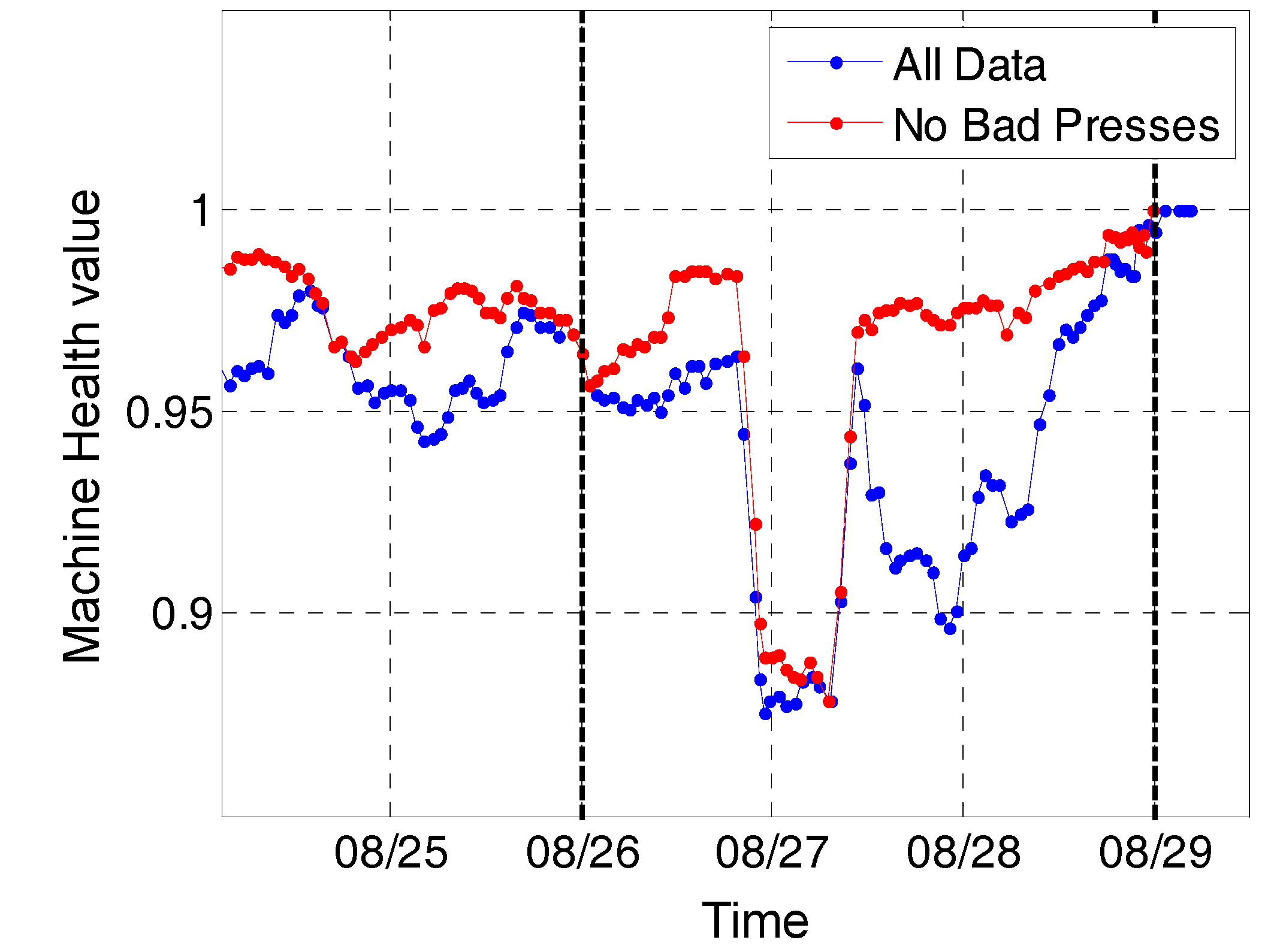
For evaluating the impact of removing the bad samples from the second stage, two metrics for the machine in the first stage were calculated: one using all the samples, and one using the remaining samples after filtering out the bad samples. Figure 4 shows both the metrics calculated for the machine in first stage. As it can be seen in this figure, removal of the samples causes the metric to bounce back to normal on 08/28, while the metric on 08/27 remained at the same level. Therefore, it is inferred that deviation observed on 08/27 is caused by the machine in the first stage, while the deviation on 08/28 is the result of performance of machines in the second stage.

4. Evaluation and Benchmarking

4.1. Data Simulation Using the Monte-Carlo Technique

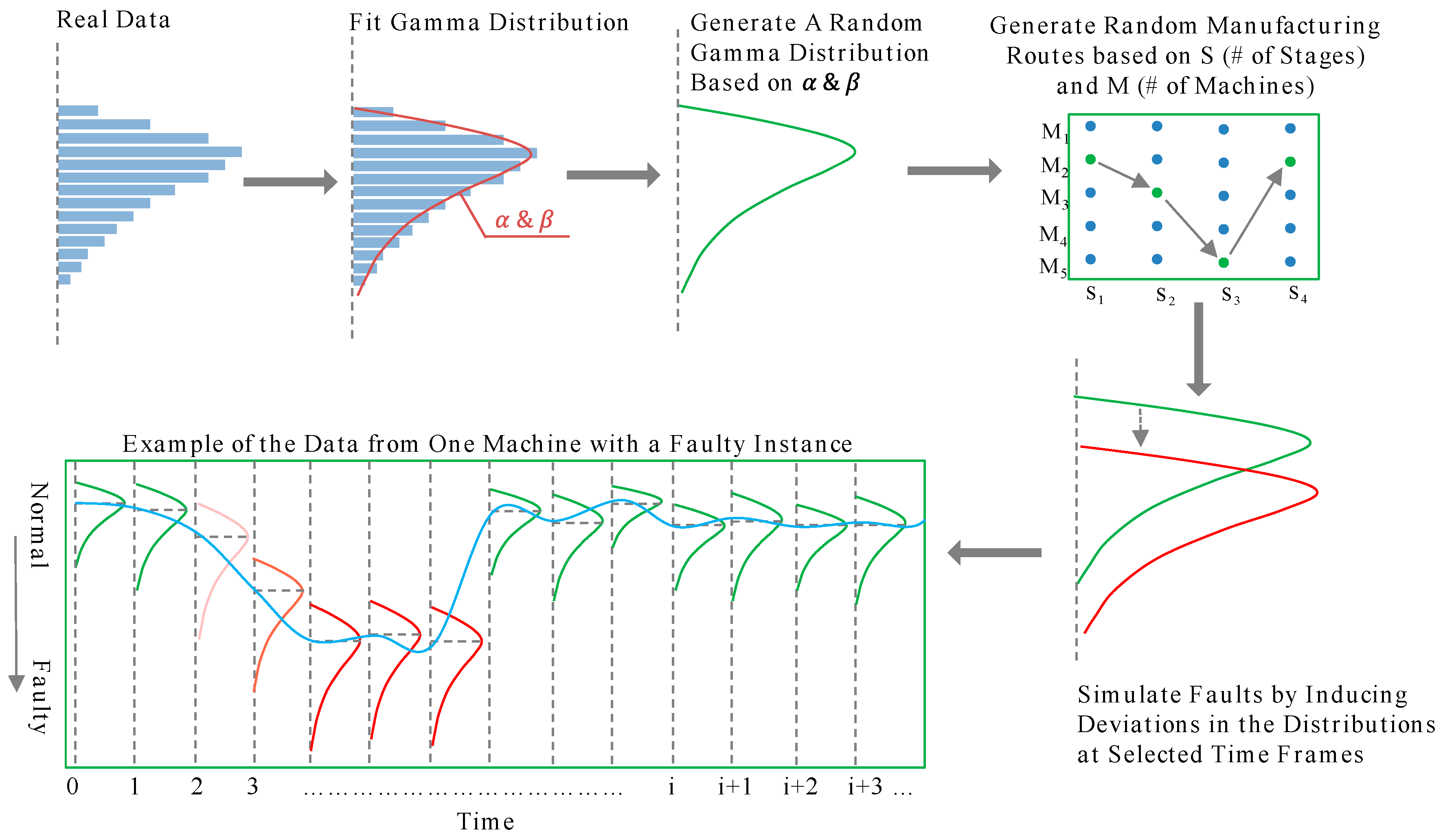
The Monte Carlo (MC) technique is a powerful tool for obtaining consistent simulation-based estimates and is comprehensively used in manufacturing applications to estimate the probability distributions for various parameters such as cutting force, tool life, product quality, etc. [26,27,28]. Monte Carlo is also used to draw a large number of samples within a distribution defined based on probability parameters [29]. In the case of simulating the data from a multistage manufacturing process, the real data—which was already available—was used to estimate the statistical parameters for data simulation, similar to how it was implemented in [30]. The procedure for simulating the data using the MC method is shown in Figure 5. A gamma distribution was fit to each of the quality variable of the data, and the shape and scale parameters of each variable were estimated. The MC simulation was programmed in MATLAB, and was developed to work for arbitrary number of machines and stages in a process. After simulating the samples for M machines and S stages, the data was time stamped and at some arbitrary instances, deviations were induced into one or more variables to simulate faulty machines. The fault instances were also randomly generated. While the total length of the simulated data was chosen to be 10 days, the fault instances lasted for two days each. The total number of faulty instances generated was dependent upon M and S, and was a number equal or close to S × M / 3 . This number ensured sufficient number of faulty instances for evaluation purposes while avoiding too many faulty machines.

4.2. Benchmark with Distribution Comparison Techniques

Statisticians have developed many tests to quantify the similarity between two distributions, which can be categorized into parametric and non-parametric tests. In parametric methods, average, standard deviation, variance etc. are used to evaluate the similarity of two distributions. In non-parametric methods, the overall distribution is considered. Due to the importance of considering the whole distribution of the parameters in this study for improved resilience of the method, non-parametric methods are more qualified to be used for benchmarking against the proposed metric calculation approach. The Kolmogorov-Smirnov (KS) test, which compares the empirical cumulative distribution functions (ECDF) of the two distributions, is a non-parametric approach and is selected as one of the benchmarking methods in this study. In a two-sample KS test, the null hypothesis is that the two samples come from the same distribution. The statistic for deriving the comparison in KS test is known as D-stat, which has the following formula [31]:
D-stat   = m a x | F 1 ( X i ) F 2 ( X i ) |     i =   1 , 2 ,   ,   N
where F 1 ( X i ) denotes the value at the i th point in the ECDF of distribution 1 and F 2 ( X i ) denotes the value at the i th point in the ECDF of distribution 2. The second method used for benchmarking in this study is Kullback-Leibler (KL) divergence technique. KL divergence, introduced in [32], is a measure of the distance between two probability distributions. Having the distributions named as P and Q, KL divergence is defined as:
D ( P | | Q ) =   x χ P ( x ) l o g P ( x ) Q ( x )
where P and Q represent the two distributions. As it can be observed from Equation (4), this metric is not symmetric. In other words, it is a directional distance and may yield substantially different values if the order of the arguments P and Q is changed. In [33], a method is proposed for symmetrizing the KL divergence metric, and the improved method is known as Jensen-Shannon (JS) divergence. Having the KL divergence in both directions named as D ( P | | Q ) and D ( Q | | P ) , the JS divergence is defined as:
J S D ( P | | Q ) = 1 2 D ( P | | Q ) +   1 2 D ( Q | | P )
In this work, the above formula is used for benchmarking against the proposed metric calculation approach. Random gamma distributions were generated based on the characteristics of the real data, and the performance of the proposed metric was evaluated against the two described methods. Four different sets of gamma distributions were generated, and for each case, the metrics were calculated:
  • Increasing the gamma distribution’s shape parameter while keeping the scale parameter more or less constant.
  • Increasing the gamma distribution’s scale parameter while keeping the shape parameter more or less constant.
  • Increasing both shape and scale parameters at the same time.
  • Linear shifting the values of one of the distributions.
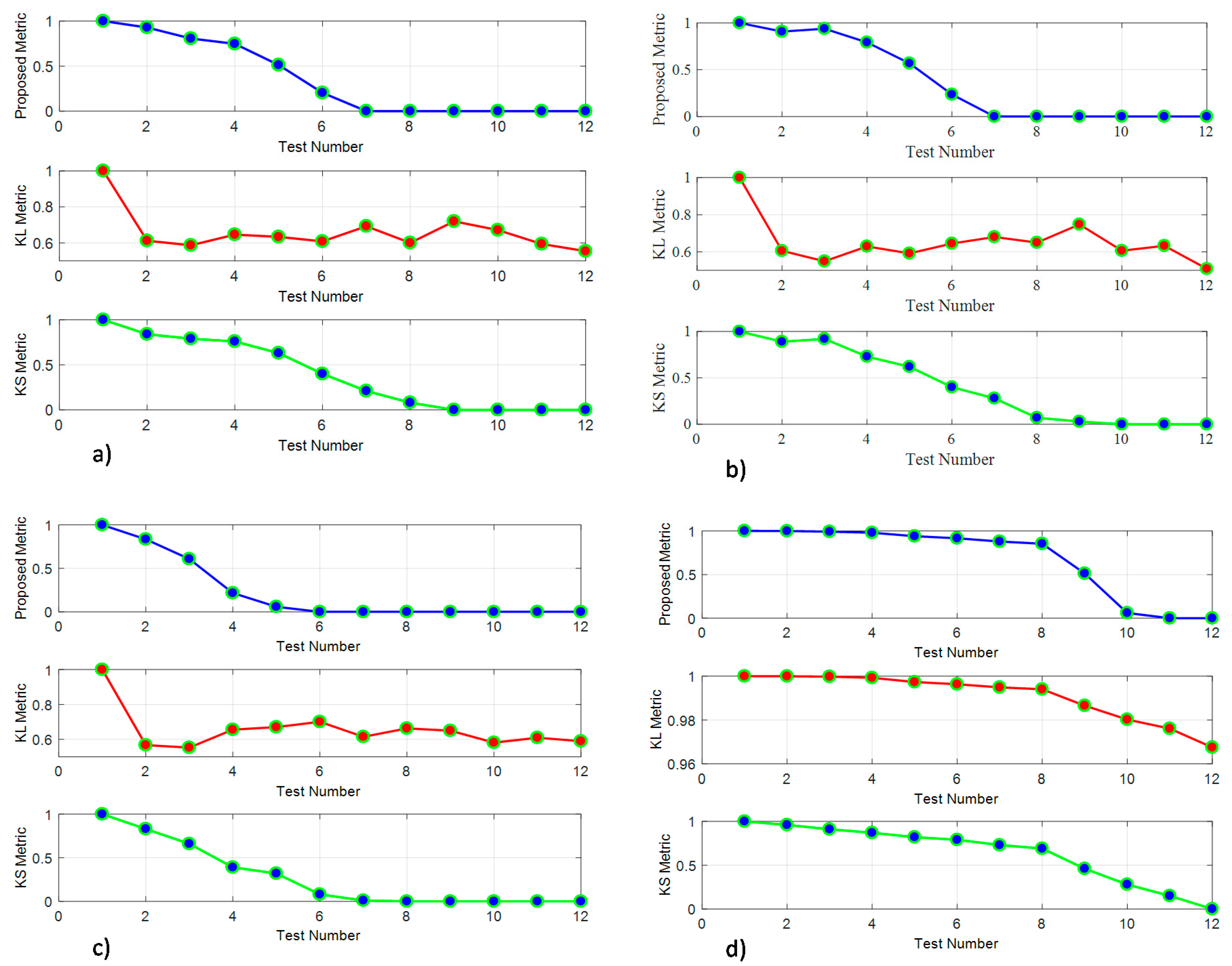
Figure 6 shows the results of the proposed metric, KL divergence and KS test statistic for the given pairs of distributions. As it can be observed from Figure 6, the proposed metric and the KS statistic both performed well in terms of early detection of the deviation and their consistency as the distributions diverge. However, the proposed metric had an advantage in terms of its consistency and its increased sensitivity compared to KS test as the divergence increases. This was observable by comparing the two metrics for test numbers 5 to 7 in Figure 6. The advantage of KL divergence method, however, was due to the fact that it shows the most sensitivity when the deviation is small. Considering that, KL divergence can be a robust method if an early alarm is desired for smallest deviations. While KL divergence had a good sensitivity in the early stages of deviation, it did not perform as consistently as the other two methods, and its values did not change consistently as the distributions diverge. The downside of implementing KL divergence is the possibility of high number of false alarms as it is very sensitive, and it fails to demonstrate the divergence trend in the data. When linearly shifting one of the distributions (Figure 6d), all the three metrics yielded similar results. Significant improvement in the performance of KL divergence metric can be observed in this case.
The results of the four tests conducted in the section demonstrate the effectiveness of the proposed metric for quantifying the deviation of a distribution under different circumstances. The KS test metric was also shown to be effective under all the conditions, with slightly less sensitivity and consistency. However, it can be considered a viable approach for quantifying the divergence of machines in a manufacturing process.

4.3. Evaluation of the Proposed Method

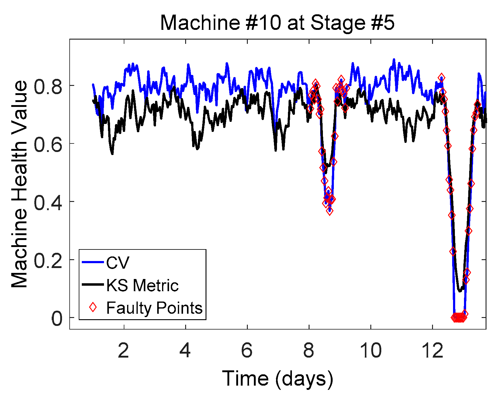
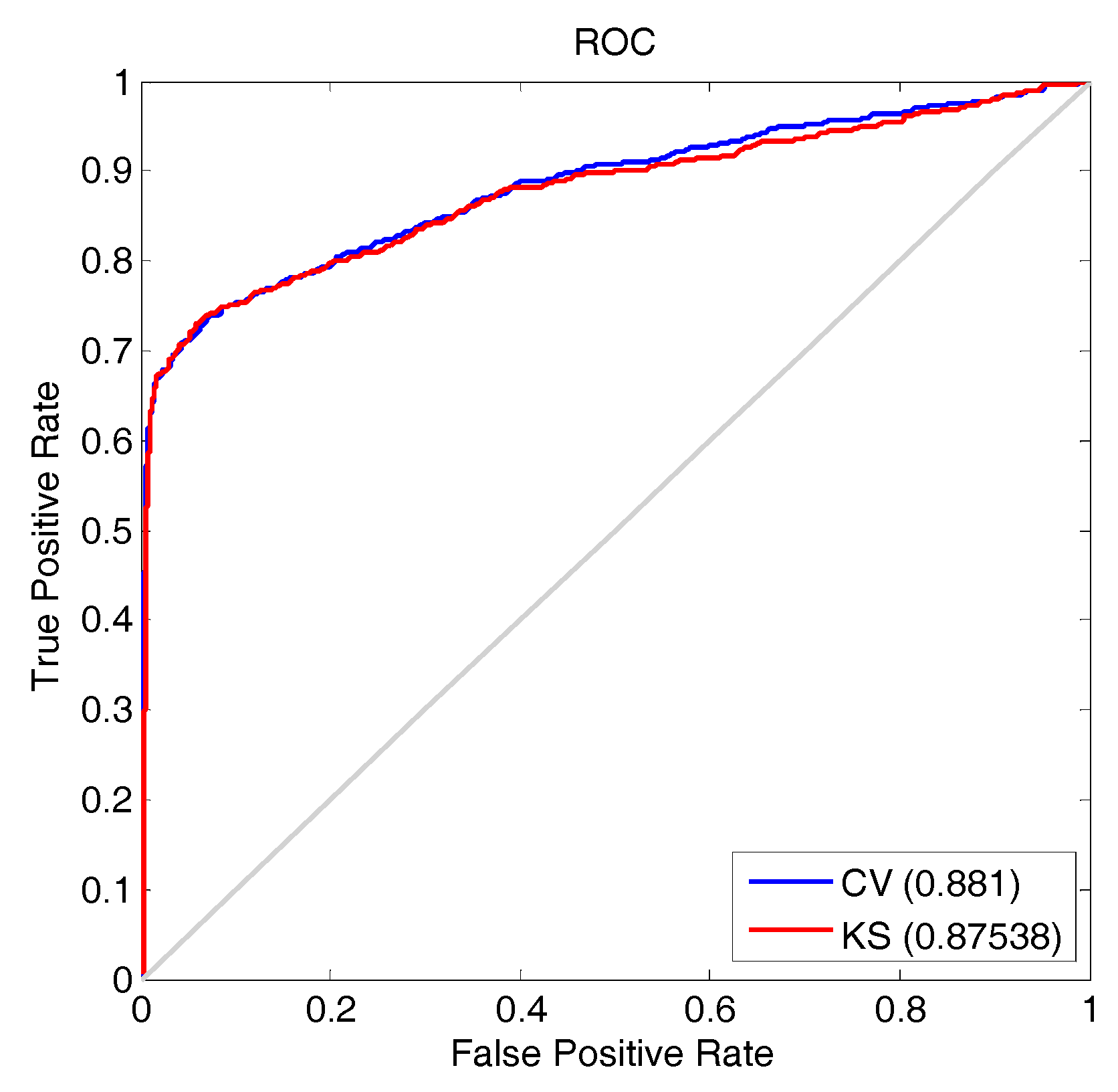
The simulated dataset was used to evaluate the performance of the proposed multistage manufacturing monitoring approach. For this purpose, a dataset was simulated consisting of five stages and 10 machines at each stage, with the duration of 15 days. The Faulty instants were induced in the data at randomly selected times for random machines with the duration of two days. A moving window with the length of 12 h and steps of 1 h was applied to the data and at each time window, the metrics were calculated. The metric calculation step was performed using both the proposed approach and KS statistic, as both proved to be effective earlier. The metric calculation started at the first stage, and it was progressed towards the end of the process while removing any instance from the previous stage detected as faulty. Figure 7 provides a machine health metric over time for one machine within a process. The results showed consistency in detecting the faults in machines regardless of which stage they are at. Figure 8 shows the Receiver Operating Characteristic (ROC) curve for fault detection using both the proposed metric and KS test statistic. Both methods resulted in high accuracy with very similar results, as the calculated area under the curves (AUC) exhibit. For all the faulty instances within the process, the method generated an alarm a few samples after the fault was initiated, which resulted in AUCs of approximately 0.9. This was due to the fact that at the early stages of a fault, a small portion of the distribution within the studied time window was faulty. That reduced the sensitivity of this method at early stages and the alarm was triggered after sufficient number of faulty samples is collected. For future work, this drawback can be eliminated by applying statistical pattern recognition techniques such as Gaussian Mixture Model (GMM) on the samples from each time window to detect smaller deviations.

4.4. The Impact of the Process Scale

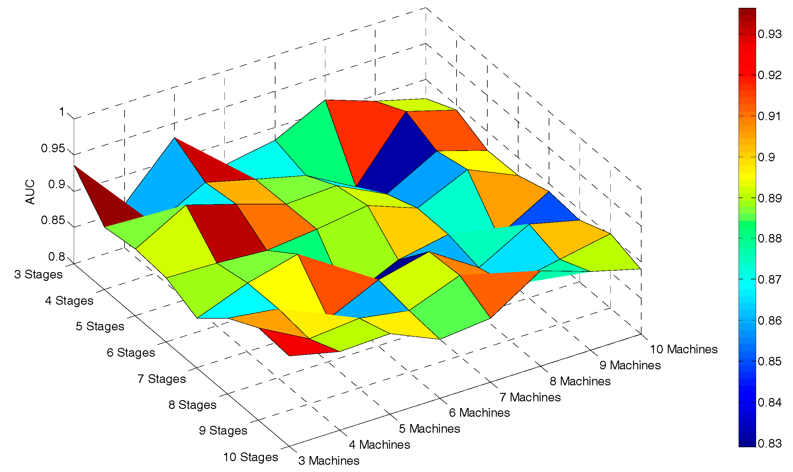
Using the simulated data, the developed similarity-based approach was evaluated in terms of the number of stages and machines within a process. For larger-scale manufacturing processes, the complexity of the process is higher and so it is more challenging to identify the root causes of variations. To evaluate the performance of the method for larger-scale manufacturing processes, the MC simulation was used to generate datasets from processes with number of stages ranging from three to 10 and number of machines ranging from three to 10, resulting in 64 datasets. Generating these sets of data facilitated the investigation of the effect of manufacturing scale on the accuracy of the method. For each dataset, the method was applied and the results were evaluated by calculating the AUC of the ROC curves. Figure 9 shows the AUC values for each of the 64 datasets. From Figure 9, it can be observed that this approach is robust for manufacturing processes with larger scales and high number of machines and stages. More importantly, the complexity and computational burden of the analysis is only increased linearly as the process scales up. In summary, it can be concluded that the proposed method is robust for different sizes of manufacturing processes and the accuracy does not get affected significantly for different numbers of machines and stages.

5. Bayesian Networks as an Alternative Method

As an alternative to the proposed similarity-based approach, a method based on implementing BN is proposed. BN is able to model the conditional relationships between the variables based on establishing posterior probabilities. Bayesian networks have been widely used for the applications of diagnostics and prognostics. For example, in [34], the authors used BN to monitor the performance of the manufacturing process for molding and welding applications. In [35], BN was utilized to analyze the process disturbance cause and effect with a case study on heat recovery networks. BN has also been used to estimate process control parameters in multistage manufacturing processes, as it was reported in [36]. A comprehensive overview of BN with its application in diagnostics and prognostics is provided in [37].
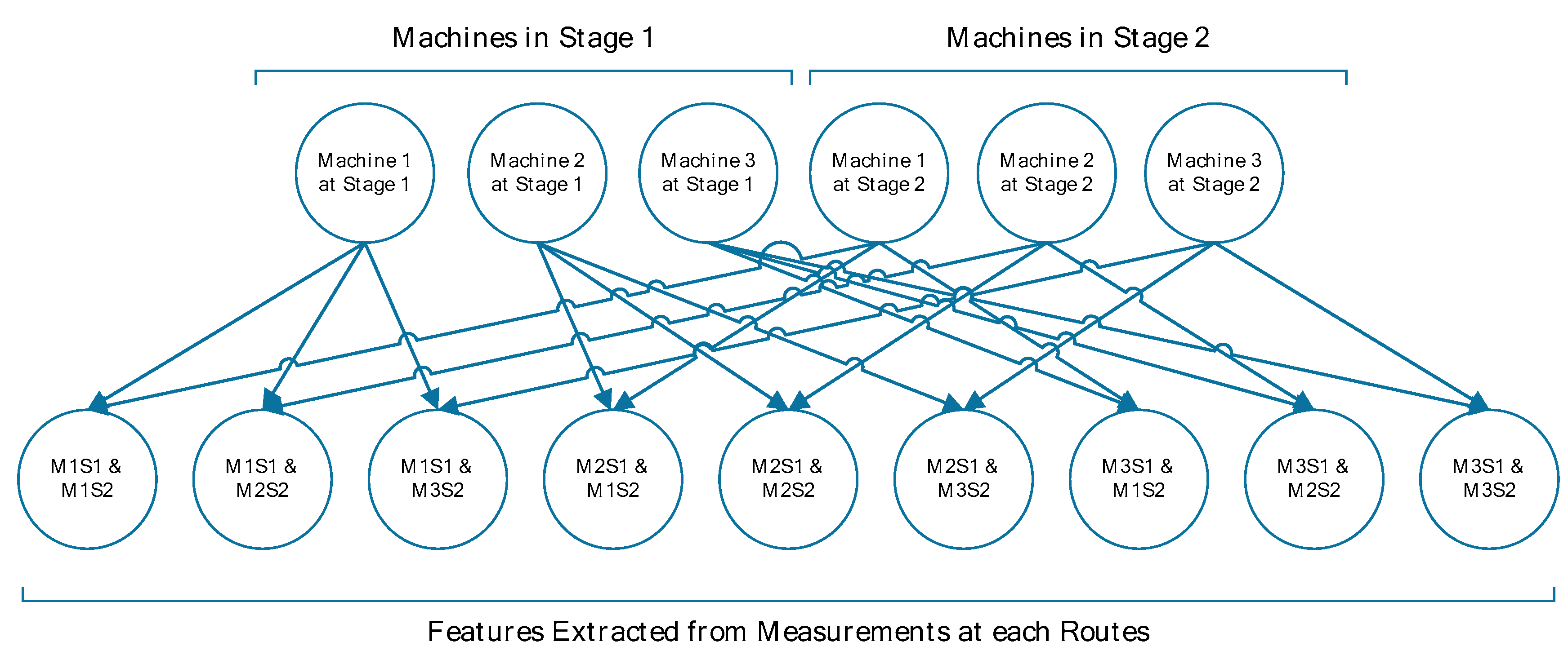
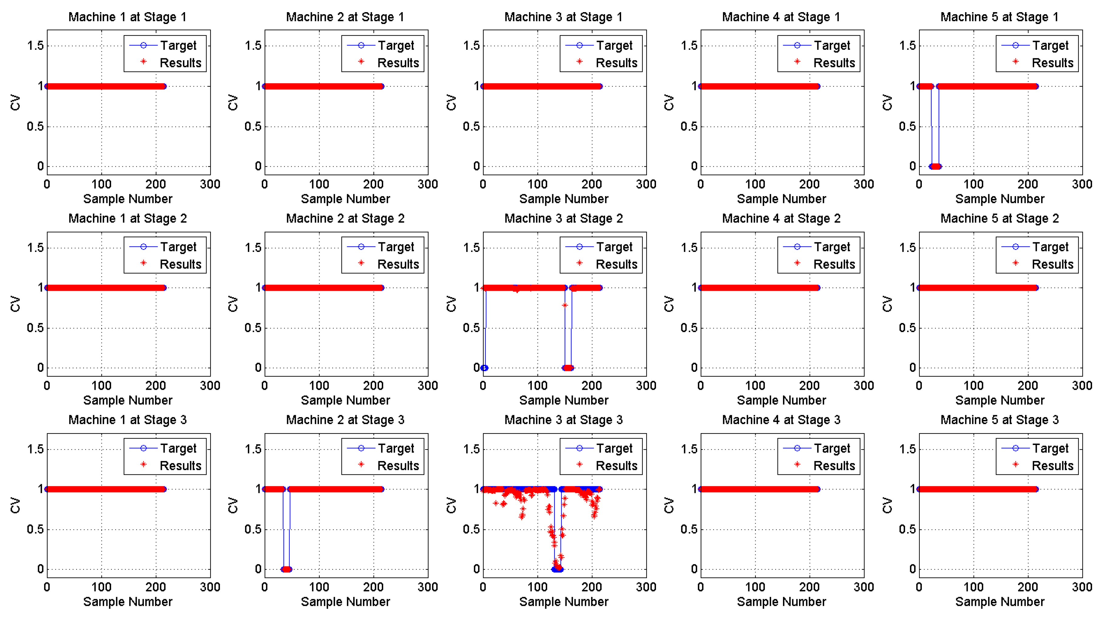
The relationships or dependencies between the variables in a BN are established either through knowledge about variables, or through the available data. As opposed to the reported works in literature—a few of which are noted above—the scope of the methods considered in this paper is only based on product quality data. Unless there is application-specific information available on the relationships between the machine performance and certain quality variables, the structure of the BN can best be established as shown in Figure 10. The structure of the BN used in this study, as shown in Figure 10, consists of a set of parent nodes each representing one machine, and a set of child nodes each representing one possible manufacturing route. The values assigned to the parent nodes consisted of machine binary conditions, and the values assigned to child nodes consisted of statistical features such as mean and standard deviation extracted from samples within each time window. Figure 11 shows the results obtained by BN for a process with three stages and five machines per stage. As it can be observed from this figure, the method is able to accurately detect the faults even at the very early stages of the fault. The AUC for this set of results was 0.96.
While this structure was shown to be effective for solving such problem, it becomes increasingly complicated as the dimensions of the manufacturing process, and especially the number of stages increase. The example shown in Figure 10 is for a process with two stages and three machines per stage. The BN structure, therefore, consisted of six parent nodes (for six machines) and nine child nodes (number of possible routes). For a process with three stages and 10 machines per stage, these numbers would be 30 and 1000 respectively. In such scales, BN may not work efficiently and the computational burden increases dramatically, and so the method may not be a suitable choice for real-time process monitoring purposes. On the other hand, for smaller-scale manufacturing processes, BN shows to be very effective and capable of identifying the patterns within the process. In this study, the largest process scale for which BN worked effectively was a three-stage process with five machines per stage. However, the similarity-based method’s performance did not drop even at larger process scale.

6. Summary and Conclusions

In this paper, a comprehensive overview of the proposed multistage manufacturing process monitoring approach was provided along with its evaluation using simulated datasets. Moreover, an alternative framework using BN was presented and proved to be effective. For demonstration and validation of the method, multiple datasets with similar characteristics as the available real-world data were generated using MC simulation technique. The MC method facilitated a more comprehensive evaluation of the performance of this method for different types of deviations in the manufacturing process data and different manufacturing scales. The current section summarizes the results obtained from analyzing the simulated datasets and provides further discussions mainly from industrial implementation perspective.
For the metric development approach, it was shown that the proposed method has adequate sensitivity and consistency for any type of deviations in the measurement distributions. This study mainly focused on sample populations that follow a gamma distribution. Using the same data simulation and analysis approach, other distributions can also be tested to see if the method is robust enough to work for a wider range of applications. In terms of comparing to other available distribution comparison techniques, two well-known methods namely KS test statistic and KL divergence method (modified by Jensen and Shannon) were utilized. Although all three methods were able to detect the deviations in the distributions, the proposed method and KS test statistic proved to be more effective both in terms of consistency and sensitivity. The proposed metric calculation technique quantifies the differences in two PDF functions both in terms of their distance and overlap, while KS statistic quantifies the maximum distance of Empirical CDF functions. Although implementing the proposed metric yielded a narrowly higher accuracy for machine anomaly detection, the KS statistic can also be considered a viable alternative to the proposed method.
Using BN is also a viable option for monitoring manufacturing processes using product quality data. In this study, BN was shown to be accurate and sensitive to process deviations. It is particularly effective and suitable for smaller-scale manufacturing units. However, the BN-based method presented in this paper is not a proper solution for larger-scale processes, and its complexity increases exponentially as the process scale increases. For larger scale manufacturing units, the similarity-based framework with less computational burden is considered the best choice, especially when real-time monitoring is concerned.

Author Contributions

Hossein Davari Ardakani analyzed the data and wrote the paper. Jay Lee advised the project and provided feedback on the methodology and data analysis.

Conflicts of Interest

The authors declare no conflict of interest.

References

  1. Djurdjanovic, D.; Mears, L.; Niaki, F.A.; Haq, A.U.; Li, L. State of the Art Review on Process, System, and Operations Control in Modern Manufacturing. J. Manuf. Sci. Eng. 2017. [Google Scholar] [CrossRef]
  2. Ceglarek, D.; Shi, J. Fixture failure diagnosis for autobody assembly using pattern recognition. J. Eng. Ind. 1996, 118, 55–66. [Google Scholar] [CrossRef]
  3. Shu, L.; Tsung, F. Multistage process monitoring and diagnosis. In Proceedings of the 2000 IEEE International Conference on Management of Innovation and Technology (ICMIT 2000), Singapore, 12–15 November 2000. [Google Scholar]
  4. Chen, T.; Zhang, J. On-line multivariate statistical monitoring of batch processes using Gaussian mixture model. Comput. Chem. Eng. 2010, 34, 500–507. [Google Scholar] [CrossRef] [Green Version]
  5. Tsung, F.; Li, Y.; Jin, M. Statistical process control for multistage manufacturing and service operations: A review. In Proceedings of the IEEE International Conference on Service Operations and Logistics, and Informatics (SOLI’06), Shanghai, China, 21–23 June 2006. [Google Scholar]
  6. Wolbrecht, E.; D’ambrosio, B.; Paasch, R.; Kirby, D. Monitoring and diagnosis of a multistage manufacturing process using Bayesian networks. Ai Edam 2000, 14, 53–67. [Google Scholar] [CrossRef]
  7. Zhou, S.; Ding, Y.; Chen, Y.; Shi, J. Diagnosability study of multistage manufacturing processes based on linear mixed-effects models. Technometrics 2003, 45, 312–325. [Google Scholar] [CrossRef]
  8. Zhou, S.; Huang, Q.; Shi, J. State space modeling of dimensional variation propagation in multistage machining process using differential motion vectors. IEEE Trans. Robot. Autom. 2003, 19, 296–309. [Google Scholar] [CrossRef]
  9. Shi, J.; Zhou, S. Quality control and improvement for multistage systems: A survey. IIE Trans. 2009, 41, 744–753. [Google Scholar] [CrossRef]
  10. Ceglarek, D.; Shi, J.; Wu, S. A knowledge-based diagnostic approach for the launch of the auto-body assembly process. J. Manuf. Sci. Eng. 1994, 116, 491–499. [Google Scholar] [CrossRef]
  11. Hu, S.J.; Wu, S. Identifying sources of variation in automobile body assembly using principal component analysis. Trans. NAMRI/SME 1992, 20, 311–316. [Google Scholar]
  12. Liu, S.C.; Hu, S.J. Variation simulation for deformable sheet metal assemblies using finite element methods. J. Manuf. Sci. Eng. 1997, 119, 368–374. [Google Scholar] [CrossRef]
  13. Lucas, J.M.; Saccucci, M.S. Exponentially weighted moving average control schemes: Properties and enhancements. Technometrics 1990, 32, 1–12. [Google Scholar] [CrossRef]
  14. Montgomery, D.C. Introduction to Statistical Quality Control; John Wiley & Sons: Hoboken, NJ, USA, 2007. [Google Scholar]
  15. Neubauer, A.S. The EWMA control chart: Properties and comparison with other quality-control procedures by computer simulation. Clin. Chem. 1997, 43, 594–601. [Google Scholar] [PubMed]
  16. Page, E. Continuous inspection schemes. Biometrika 1954, 41, 100–115. [Google Scholar] [CrossRef]
  17. Rato, T.J.; Reis, M.S. Statistical Process Control of Multivariate Systems with Autocorrelation. In Computer Aided Chemical Engineering; Elsevier: Amsterdam, The Netherlands, 2011; pp. 497–501. [Google Scholar]
  18. Reynolds, M.R.; Amin, R.W.; Arnold, J.C.; Nachlas, J.A. Charts with variable sampling intervals. Technometrics 1988, 30, 181–192. [Google Scholar] [CrossRef]
  19. Reynolds, M.R.; Amin, R.W.; Arnold, J.C. CUSUM charts with variable sampling intervals. Technometrics 1990, 32, 371–384. [Google Scholar] [CrossRef]
  20. Roberts, S. Control chart tests based on geometric moving averages. Technometrics 1959, 1, 239–250. [Google Scholar] [CrossRef]
  21. Hu, S.J.; Koren, Y. Stream-of-variation theory for automotive body assembly. CIRP Ann. Manuf. Technol. 1997, 46, 1–6. [Google Scholar] [CrossRef]
  22. Shi, J. Stream of Variation Modeling and Analysis for Multistage Manufacturing Processes; CRC Press: Boca Raton, FL, USA, 2010. [Google Scholar]
  23. Woodall, W.H.; Montgomery, D.C. Some current directions in the theory and application of statistical process monitoring. J. Qual. Technol. 2014, 46, 78. [Google Scholar] [CrossRef]
  24. Cheng, S.; Azarian, M.H.; Pecht, M.G. Sensor systems for prognostics and health management. Sensors 2010, 10, 5774–5797. [Google Scholar] [CrossRef] [PubMed]
  25. Ardakani, H.D.; Phillips, B.; Bagheri, B.; Lee, J. A New Scheme for Monitoring and Diagnosis of Multistage Manufacturing Processes Using Product Quality Measurements. In Proceedings of the Annual Conference of the Prognostics and Health Management Society, Coronado, CA, USA, 18–24 October 2015. [Google Scholar]
  26. Karandikar, J.M.; Abbas, A.E.; Schmitz, T.L. Tool life prediction using Bayesian updating. Part 2: Turning tool life using a Markov Chain Monte Carlo approach. Precis. Eng. 2014, 38, 18–27. [Google Scholar]
  27. Niaki, F.A.; Ulutan, D.; Mears, L. Parameter inference under uncertainty in end-milling γ′-strengthened difficult-to-machine alloy. J. Manuf. Sci. Eng. 2016, 138, 061014. [Google Scholar] [CrossRef]
  28. Gözü, E.; Karpat, Y. Uncertainty analysis of force coefficients during micromilling of titanium alloy. Int. J. Adv. Manuf. Technol. 2017, 93, 839–855. [Google Scholar] [CrossRef]
  29. Siegel, D.; Lee, J. An Auto-Associative Residual Processing and K-Means Clustering Approach for Anemometer Health Assessment. In International Journal of Prognostics and Health Management Volume 2; Lulu Press, Inc.: Morrisville, NC, USA, 2011. [Google Scholar]
  30. Doucet, A.; Wang, X. Monte Carlo methods for signal processing: A review in the statistical signal processing context. IEEE Signal Process. Mag. 2005, 22, 152–170. [Google Scholar] [CrossRef]
  31. Kar, C.; Mohanty, A. Application of KS test in ball bearing fault diagnosis. J. Sound Vib. 2004, 269, 439–454. [Google Scholar] [CrossRef]
  32. Kullback, S.; Leibler, R.A. On information and sufficiency. Ann. Math. Stat. 1951, 22, 79–86. [Google Scholar] [CrossRef]
  33. Johnson, D.; Sinanovic, S. Symmetrizing the kullback-leibler distance. Available online: https://scholarship.rice.edu/bitstream/handle/1911/19969/Joh2001Mar1Symmetrizi.PDF?sequence=1&isAllowed=y (accessed on 15 December 2017).
  34. Nannapaneni, S.; Mahadevan, S.; Rachuri, S. Performance evaluation of a manufacturing process under uncertainty using Bayesian networks. J. Clean. Prod. 2015, 113, 947–959. [Google Scholar] [CrossRef]
  35. Leng, D.; Thornhill, N.F. Process Disturbance Cause & Effect Analysis Using Bayesian Networks. IFAC-PapersOnLine 2015, 48, 1457–1464. [Google Scholar]
  36. Du, S.; Yao, X.; Huang, D. Engineering model-based Bayesian monitoring of ramp-up phase of multistage manufacturing process. Int. J. Prod. Res. 2015, 53, 4594–4613. [Google Scholar] [CrossRef]
  37. Zhao, W. A Probabilistic Approach for Prognostics of Complex Rotary Machinery Systems. Ph.D. Thesis, University of Cincinnati, Cincinnati, OH, USA, 2015. [Google Scholar]
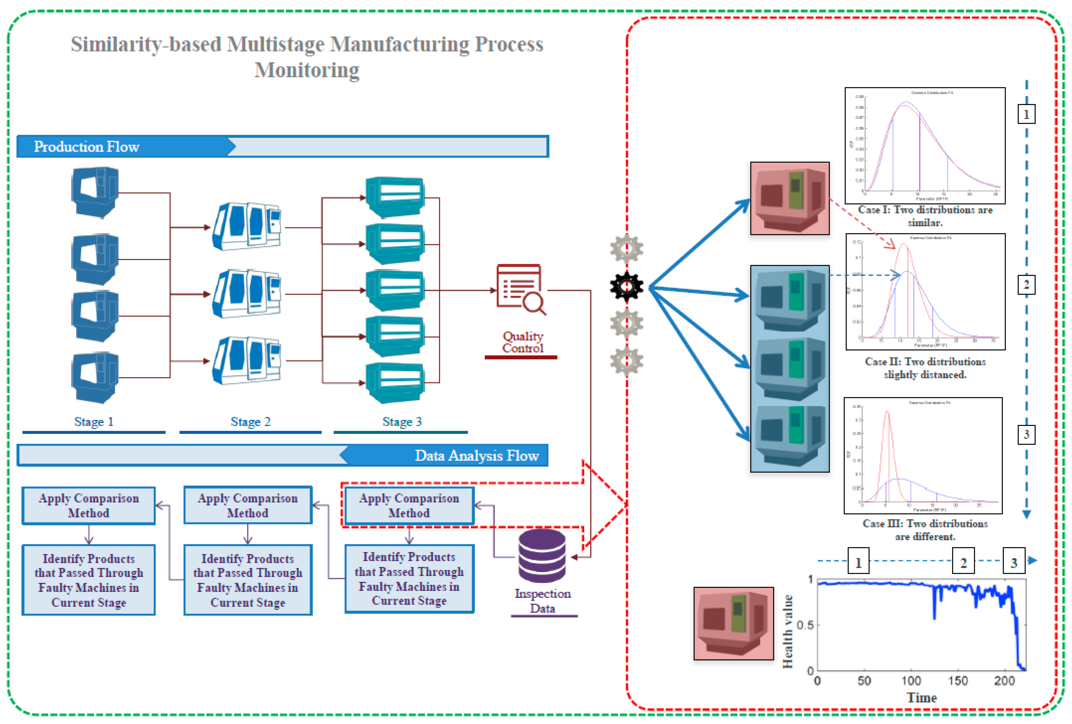
Figure 1. The proposed framework for similarity-based multistage manufacturing process monitoring using product quality data [25].
Machines 06 00001 g001
Figure 2. Examples of the metrics calculated within one time window: (a) two significantly different distributions yielding a CV of close to 0.2; (b) two distributions yielding a CV of around 0.5; (c) two very similar distributions yielding a CV of close to 1 [25]. Red curve shows the distribution of the selected machine and blue curve shows the distribution of its peers. Green line shows the selected area for calculating the CV.
Machines 06 00001 g002
Figure 3. Calculated CV for three machines in stage 2 producing the same type of product [26].
Machines 06 00001 g003
Figure 4. Calculated CV for the machine in stage 1 before removing the samples from stage 2 (blue) and after removing the samples from stage 2 (red) [25].
Machines 06 00001 g004
Figure 5. The process of using the Monte-Carlo simulation for generating data from a manufacturing process with arbitrary number of stages and machines.
Machines 06 00001 g005
Figure 6. The results of the three metrics calculated based on: (a) changing the shape parameter of a gamma distribution; (b) changing the scale parameter of a gamma distribution; (c) changing the shape and scale parameters of gamma distribution; (d) linearly shifting the distribution.
Machines 06 00001 g006
Figure 7. The calculated health value for a machine in a process with five stages and ten machines per stage. The results using the proposed metric (CV) and KS metric are compared. Red markers represent faulty samples.
Machines 06 00001 g007
Figure 8. The ROC curve for results calculated using the proposed method and KS statistic as metric.
Machines 06 00001 g008
Figure 9. The calculated area under the curves (AUC) for processes with different number of stages and different number of machines per stage.
Machines 06 00001 g009
Figure 10. A sample Bayesian Network (BN) structure for a process with two stages and three machines at each stage; each parent node represents a machine and each child node represents the measurements from one route. “M” here stands for machine and “S” stands for stage e.g., M1S1 stands for machine 1 from stage 1.
Machines 06 00001 g010
Figure 11. The results of the BN for monitoring and diagnosis of a multistage manufacturing process with three stages and five machines per stage.
Machines 06 00001 g011