Optimization of Microchannel Heat Sinks Using Prey-Predator Algorithm and Artificial Neural Networks

Abstract

A rectangular microchannel heat sink is modeled by employing thermal resistance and pressure drop networks. The available correlations for both thermal resistance and pressure drop are utilized in optimization. A multi-objective optimization technique, the prey–predator algorithm, is employed with the objective to find the optimal values for the heat sink performance parameters, i.e., thermal resistance and the pumping power of the heat sink. Additionally, a radial basis function neural network is used to investigate a relationship between these parameters. Full training based on the prey–predator algorithm with the sum of the squared error function is used to achieve the best performance of the model. The analysis of variance method is also employed to test the performance of this model. This study shows that the multi-objective function based on the prey–predator algorithm and the neural networks is suitable for finding the optimal values for the microchannel heat sink parameters. The minimum values of the multi-objective function are found to be “pumping power = 2.79344” and “total thermal resistance = 0.134133”.

1. Introduction

These days, the size of electronic devices is reducing, whereas the power density is growing continuously. Consequently, the electronics industry is facing the thermal management problems. Microchannels provide a cooling solution for these problems and have been used in several cooling techniques, heat exchangers, bioengineering, and drug engineering [1,2,3,4]. Following Tuckerman and Pease [5], Zhang et al. [6] extended the use of microchannels to solve thermal management problems. Later, several researchers including [7,8,9,10,11] used microchannel heat sinks to reduce hydraulic and thermal resistance to improve the overall performance of chips and other electronic devices. Pin-fin structures and micro pin-fins were also used to enhance the performance of microchannel heat sinks [12,13,14,15,16].

An optimization problem consists of a single or multi-objective function with corresponding decision variables to optimize the functions [17,18]. Its importance in engineering is fundamental to execute the task concerning finding the optimal solution. Metaheuristic algorithms are optimization algorithms which try to improve the quality of initial (pseudo-) randomly-generated solutions through iteration. The prey–predator algorithm (PPA) is a metaheuristic algorithm, introduced by Tilahun and Ong [17]. It is inspired by the interaction between a predator and prey of animals in an ecosystem. The algorithm has been found to be effective when applied to different problems, including radial basis function neural networks (RBFNNs), weight minimization of a speed reducer, a bi-level problem model of an electricity market, parameter setting of a grinding process, and single-frequency bus timetabling [19,20,21,22]. It has also been modified to suit combinatorial optimization problems, like the travel salesman problem, both the standard and clustered traveling salesman problems, and exam timetabling problem [23]. Furthermore, to boost its performance it has been extended to different versions [24]. In order to increase controlling the degree of exploration and exploitation a new version is introduced [25]. Adaptive step length incorporation is another idea to extend the algorithm to obtain a good approximate result. Comparative study shows that its performance is good and it is a also generalized swarm-based algorithm where firefly algorithms, the gravitational search algorithm, and random search are the special cases of this algorithm [26,27].

An artificial neural network (ANN) is one of the artificial inelegance applications [28]. It has recently been used widely to model human interesting activities in many scopes. The discipline of neural networks is well developed with wide applications in almost all areas of science [22,29,30,31]. RBFNN is a feed-forward neural network and has been widely applied in many fields. It is different from the other neural networks, which possess several distinctive features. Owing to its universal approximation ability, it is more compact topology and faster learning speed.

In this study, RBFNN is used to construct a model for investigating a relationship between the total thermal resistance and the pumping power. Additionally, we have used multi-objective optimization (also known Pareto optimization), and a set of solutions of optimal values of total thermal resistance, and the pumping power of the heat sink, which depends upon the overall pressure drop in the heat sink, is obtained. The weighting method is used for obtaining multiple solutions from the Pareto front, which include better accuracy when compared to classical methods like ideal point method. Consequently, the present study is about the optimization of multi-objective functions using PPA to determine the optimal values of total thermal resistance and the pumping power. In the next section, a literature review related to entropy generation and optimization is described.

2. Literature Review

Several theoretical, numerical, and experimental studies related to the optimization of microchannel heat sinks have been reported in the literature. Khan et al. [32] employed an entropy generation minimization method to optimize the overall performance of microchannel heat sinks. They used existing analytical/empirical correlations for heat transfer and friction coefficients and performed parametric studies to show the effects of different design variables on the overall performance of microchannel heat sinks. Abbassi [33] analyzed entropy generation in a uniformly-heated microchannel heat sink. He considered second law of thermodynamics and derived expressions for local and average entropy generation rates in dimensionless form. He investigated the effect of influential parameters on local and total entropy generation. Adham et al. [34] considered the entropy generation minimization (EGM) as a single-objective function and minimized entropy using a genetic algorithm (GA) for a rectangular microchannel heat sink. They conducted a parametric study to examine the overall performance under laminar and turbulent flow conditions. Chen [35] employed the second law of thermodynamics to investigate the entropy generation in a microchannel for different thermal boundary conditions. It was demonstrated that the convection effect on entropy and fluid temperature is negligible for small Peclet numbers. Li and Kleinstreuer [36] performed entropy generation analysis in a trapezoidal microchannel heat sink. They considered two particle volume fractions (1% and 4%) in the laminar flow region and discovered that there exists an optimum Reynolds number range for the maximum performance of microchannel heat sinks (MCHs).

Adham et al. [37] presented a comprehensive review of available studies related to enhancing overall thermal and hydrodynamic performance of rectangular microchannel heat sinks. They analyzed and optimized the overall performance of microchannel systems with reference to different parameters. They found that the current studies show a dependency on numerical simulations and evolutionary algorithms. Wang et al. [38] employed an inverse problem method to optimize the geometric design for microchannel heat sinks using a novel multi-parameter optimization approach. They minimized the overall thermal resistance with number of channels, channel aspect ratio, and the ratio of channel width to pitch. They found that an increase in the pumping power reduces overall thermal resistance of the optimal design. Karathanassis et al. [39] employed GA to optimize a micro heat sink. They considered two different microchannel configurations and optimized the thermal resistance of the heat sink and the cooling medium pressure drop through the heat sink. They demonstrated that heat sinks achieve very low values of thermal resistance. Ndao et al. [40] utilized a multi-objective GA to determine the optimal thermal design based on the total thermal resistance and pumping power consumption under a constant pressure drop. They noticed a trade-off between the overall thermal resistance and pumping power consumption. Normah et al. [41] employed a multi-objective GA and obtained the optimal values of the hydraulic diameter and wall width to channel width ratio of both square and circular microchannel heat sinks. They found that with the same hydraulic diameter and pumping power, circular microchannels have lower thermal resistance. Khan et al. [42] employed GA to minimize the entropy generation rate in microchannel heat sinks. They demonstrated that the genetic algorithm gives better overall performance of the microchannel heat sinks.

Shao et al. [43] optimized the shape and size of rectangular microchannels cooling heat sink using the sequential quadratic programming (SQP) method. They found that the heat transfer performance of microchannel cooling heat sink is affected intensively by both shape and size of he microchannel. Later, Shao et al. [44] optimized a multi-layer microchannel heat sink by considering the thermal resistance and the pressure drop as goal functions. They proposed a double-objective optimization model based on the thermal resistance network model and used computational fluid dynamics (CFD) software for numerical simulations. Knight et al. [45] presented a scheme for solving dimensionless equations for both laminar and turbulent flows in a microchannel heat sink. They found that, for a small pressure drop through the channels, laminar solutions give lower thermal resistance than turbulent solutions. Using this fact, they produced a significant improvement in thermal resistance. Hu and Xu [46] proposed a nonlinear, single-objective, and multi-constrained optimization model for the cooling of electronic chips using the SQP method. They found that the heat transfer performance of the microchannel heat sink depends upon its dimensions. Dede [47] employed a multi-physics topology optimization method to optimize and design a multi-pass branching microchannel heat sink for high heat flux electronic cooling applications. He found that the derived cold plate exhibits favorable heat transfer with a low-pressure drop due to multiple passes through the branching microchannel. Hussain and Kim [48] carried out a numerical investigation of three-dimensional (3-D) fluid flow and heat transfer in a rectangular microchannel. They optimized the shape of the microchannel using sequential quadratic programming, response surface approximation, kriging, and radial basis neural network methods. Kou et al. [49] developed a 3-D numerical model of the microchannel heat sink to optimize the effects of heat transfer characteristics due to various channel heights and widths. They obtained the minimum thermal resistance and optimal channel dimensions by using the simulated annealing method. Kleiner et al. [50] investigated theoretically, and experimentally, a high-performance forced air cooling scheme for microchannel parallel plate-fin heat sinks. They optimized the dimensions of a microchannel heat sink and obtained optimal values of thermal resistance, pressure drop, and pumping power. Yang et al. [30] compared and discussed the flow and thermal modeling of different heat sinks. They developed a general process for optimization and performed numerical calculations.

3. Microchannel Heat Sinks

The geometry of a microchannel heat sink is shown in Figure 1. The length and width of the heat sink are assumed to be L and W, respectively. The thickness of the base surface is t_b. It is assumed that the top surface is insulated and uniform heat flux q_w is applied at the bottom surface. Air passes through n rectangular microchannels along the x-axis and takes heat away. It is assumed that each channel has a height H_c and width w_c. The thickness of each fin is w_w. The temperature of the base surface is supposed to be T_b with an ambient temperature of T_a. The assumed values of parameters and operating conditions are reported in

Table 1. Assumed operating conditions.

Operating Conditions	Assumed Values	Operating Conditions	Assumed Values
Length of MCH, L (mm)	51	Specific heat of air (kJ/kg·K)	1.007
Width of MCH, W (mm)	51	Kinematic viscosity (m2/s)	1.58 × 10−5
Channel height, Hc (mm)	1.7	Prandtl number of air	0.71
Thermal conductivity of MCH (W/m·K)	148	Heat flux (W/cm2)	15
Thermal conductivity of air (W/m·K)	0.0261	Volume flow rate (m3/s)	0.007
Density of air (kg/m3)	1.1614	Ambient temperature (K)	300

.

Following assumptions were employed in modeling:

1. Fin tips are adiabatic.

2. Heat and fluid flow are fully developed.

3. The flow is steady, laminar and 2-D.

4. The fluid is incompressible, and the thermophysical properties are constant.

5. Axial conduction is negligible in both the fin and fluid.

6. The contact between fin and base plate is perfect.

3.1. Thermal Resistance Model

The total thermal resistance of the microchannel heat sink is defined as:

$$R_{tot}=\frac{T_b-T_a}{q_w}$$

(1)

where T_b is the base temperature of microchannel heat sink and T_a is the ambient temperature. The total thermal resistance can also be written as shown in Figure 2 or as in Equation (2).

$$R_{tot}=R_{\mathrm{cond}}+R_{\mathrm{conv}}+R_{\mathrm{fluid}}+R_{\mathrm{cons}}$$

(2)

where $R_{\mathrm{cond}},R_{\mathrm{conv}},R_{\mathrm{fluid}}\mathrm{and} R_{\mathrm{cons}}$ are the conductive, convective, fluid, and constrictive thermal resistances and are given by [32,50,51].

$$\begin{gathered} R_{\mathrm{cond}}=\frac{t_b}{WL{K}_{\mathrm{w}}} \\ {R}_{\mathrm{conv}}=\frac{1}{WL{H}_{\mathrm{av}}A} \\ {R}_{\mathrm{fluid}}=\frac{1}{\dot{m}{C}_{\mathrm{p}}} \\ {R}_{\mathrm{cons}}=\frac{(w_{\mathrm{W}}+w_c)}{\pi K_{w}WL}\ln \left[\frac{1}{\sin \frac{\pi w_w}{2(w_w+w_c)}}\right] \end{gathered}$$

(3)

where k_w is the thermal conductivity of the heat sink, h_av is the average heat transfer coefficient, $\dot{m}$ is the mass flow rate and A is the convective heat transfer area of the heat sink given by:

$$\dot{m}={\rho }_{f}G$$

$$A=nL(w_c+2\eta H_c)$$

With $n=\frac{W-w_{\mathrm{w}}}{w_c+w_{\mathrm{w}}}$, number of microchannels, $\eta =\frac{\tan \mathrm{h}(m{H}_c)}{m{H}_c}$, fin efficiency, and

$$m=\sqrt{\frac{2h_{av}}{K_w{w}_{\mathrm{w}}}}$$

(4)

Based on hydraulic diameter, Reynolds and Nusselt number can be defined as:

$$\begin{gathered} R{e}_{D_h}=\frac{U_c{D}_h}{v_f}=\frac{2G}{v_{f}n}\frac{1}{w_c+H_c} \\ N{u}_{D_h}=\frac{h_{av}{D}_h}{K_f} \end{gathered}$$

(5)

With

$$D_h=\frac{2H_c{w}_c}{H_c+w_c}$$

where U_c is the velocity of fluid in the microchannel and can be determined from the volume flow rate given by:

$$G=n{H}_c{w}_c{U}_c$$

(6)

With

$$D_h=\frac{2H_c{w}_c}{H_c+w_c}$$

where U_c is the velocity of fluid in the microchannel and can be determined from the volume flow rate given by:

$$G=n{H}_c{w}_c{U}_c$$

(6)

Following Kim and Kim [52], the Nusselt number for laminar fully-developed flow in a rectangular microchannel heat sink can be written as:

$$N{u}_{D_h}=2.253+8.164{\left(\frac{\alpha }{1+\alpha }\right)}^{1.5}$$

(7)

which gives the average heat transfer coefficient:

$$h_{av}=\frac{N{u}_{D_h}{K}_f}{2H_c}(1+\alpha )$$

(8)

3.2. Pressure Drop Model

The total pressure drop in the heat sink is associated with the power required to move the fluid across microchannel. This pressure drop dictates the hydraulic resistance of the system. Like thermal resistance, it also affects the overall performance of the heat sink. It is given by:

$$\Delta P_{tot}=\Delta P_{\mathrm{ce}}+\Delta P_{\mathrm{fric}}$$

(9)

where ΔP_ce is the pressure drop due to the abrupt contraction/expansion, and ΔP_fric is the pressure loss due to core friction (Figure 3). Following Kleiner et al. [50], these pressure drops can be written as:

$$\begin{gathered} \Delta P_{\mathrm{ce}}=\left[1.79-2.32\left(\frac{1}{1+\beta }\right)+0.53{\left(\frac{1}{1+\beta }\right)}^2\right]\frac{\rho U_c{}^2}{2} \\ \Delta P_{\mathrm{fric}}=nf\frac{L}{D_h}\frac{\rho U_c{}^2}{2} \end{gathered}$$

(10)

where n is the number of channels, U_c is the fluid velocity in the channels, and f is the friction factor. Following Phillips [53], the friction factor for the fully developed laminar flow can be written as:

$$f=\frac{24}{R{e}_{D_h}}\left(1-\frac{1.3553}{\alpha }+\frac{1.9467}{{\alpha }^2}-\frac{1.7012}{{\alpha }^3}+\frac{0.9564}{{\alpha }^4}-\frac{0.2537}{{\alpha }^5}\right)$$

(11)

With $\alpha =\frac{H_C}{W_C}$.

Once total pressure drop is known, the required pumping power can be determined as follows:

$$P_P=\Delta P_{tot}G$$

(12)

where G is the volumetric flow rate, given by Equation (6).

Using Equations (3)–(12), the total thermal heat sink resistance and pumping power can be determined as a function of air and heat sink material properties as well as heat sink geometry. For specified dimensions of the heat sink, and properties of air, and heat sink material (Table 1), the optimum design of a microchannel heat sink can be achieved by minimizing overall resistance as a function of w_c, w_w, and G.

4. Solution Approach

4.1. Prey–Predator Algorithm (PPA)

PPA is a metaheuristic algorithm developed for handling complex optimization problems. It is inspired by the interaction between a carnivorous predator and its prey. The algorithm mimics how a predator runs after and hunts its prey, where each prey tries to stay within the pack, search for a hiding place, and run away from the predator.

In the algorithm, a set of initial feasible solutions will be generated and, for each solution, x_i, is assigned a numerical value to show its performance in the objective function called survival value (SV(x_i)). Better performance in the objective function implies a higher survival value. This means for solutions x_i and x_j, if x_i performs better than x_j in the objective function, SV(x_i) > SV(x_j). A solution with the smallest survival value will be assigned as a predator, x_predator, and the rest as prey. Among these prey, a prey, say x_b, where SV(x_b) ≥ SV(x_i), for all i, is called the best prey. This means the best prey is a prey with the highest survival value among the solutions.

Once the prey and the predator are assigned, each prey needs to escape from the predator and try to follow other prey with better survival values or find a hiding place. The predator hunts the weak prey and scares the others which contribute to the exploration of the solution space. Exploitation is carried out by the preys, primarily the best prey, by using a local search. The best prey is considered as the one who has found a secure place and is safe from the predator. Thus, it will only focus on conducting a local search to improve its survival value. However, the other prey will follow the prey population with better-surviving values and run away from the predator. In the updating process of these solutions, there are two issues to deal with, the direction and the step length.

In the algorithm, the movement of an ordinary prey (not the best prey) depends on an algorithm parameter called the probability of follow up (or follow up prospect). If the follow up expectation is achieved, which is if a randomly generated number between zero and one from a uniform distribution is less than, or equal to, the probability of follow up, then the prey will follow other prey with better survival values and performs a local search; otherwise it will randomly run away from the predator.

Suppose the follow-up probability is met and there is prey with better survival values compared to x_i, say x₁, x₂, …, x_s. Mostly, a group of prey tends to stay in the pack and it tries to be with the nearest pack of prey animals. Therefore, the movement of x_i is highly dependent on the distance between itself and better prey. Hence, the direction of movement of x_i can be calculated as follows:

$$y_i={\displaystyle \sum }_j{e}^{SV{(x_j)}^v-r_{ij}}(x_j-x_i)$$

(13)

where r_ij = ||x_i − x_j|| is a distance between x_i and x_j, and v is an algorithm parameter which plays the role of magnifying or diminish the effect of the survival value over the distance.

By assigning different values of v, it is possible to adjust the dependency of the updating direction on the survival value and the distance. If v is too large, then the direction favors the performance than the distance of the better prey from the solution, this means the prey tries to catch up with the best pack with little consideration how far that pack is. If v is too small, it implies that the prey prefers to follow the nearest better pack. Assigning a large or a small value for v will affect the jump size of x_i. Hence, a unit direction will be used to represent the direction as:

$$u_i=\frac{y_i}{\Vert y_i\Vert }$$

(14)

Moreover, a local search is done by generating q random directions and taking the best direction, say y_i, among these q directions. To choose y_i the survival value will be checked if the solution moves in the q directions and the direction which results the highest survival value will be taken.

If the follow-up probability is not met, the prey will randomly run way from the predator. This is done by generating a random direction y_rand and comparing the distance between the predator and the prey if it moves in y_rand or −y_rand, and the direction which will take the prey away from the predator will be considered.

Unlike the other ordinary prey, the movement of the best prey will perform only a local search. It will just move towards the direction which can improve its survival value, from a randomly generated q direction, or it stays in its current position if no such path exists among the q unit directions.

In the algorithm, the primary task of the predator is to motivate the prey for exploring the solution space, and it also does the exploration of the solution spaces. Thus, it will chase after the prey with the lowest survival value and moves randomly in the solution space. Hence, the movement direction will have two components: random direction, as well as towards the weak prey, x’.

Step length is the other issue related to the updating of solutions. In the carnivorous predation, a prey which is near to the predator runs faster than other preys. A similar concept is mimicked in such a way that a prey with small survival value runs more quickly than a more critical survival valued prey. Therefore, a prey has a step length λ that is inversely proportional to its survival value. This can be expressed as the following formulation:

$$\lambda =\frac{{\lambda }_{max}rand}{{|SV(x_i)-SV(x_{predator})|}^w}$$

(15)

where r_and is a random number from a uniform distribution, 0 ≤ r_and ≤ 1 and $\lambda$_max represents the size of the maximum jump of a prey. Parameter w influences the dependency of the step length on the relative survival value. However, for practical purposes, it is also possible to omit the effect of the survival value in assigning the maximum jump, which eliminates the further study of changes in survival values to choose the parameter w. Hence, we can just have:

$$\lambda ={\lambda }_{max}rand$$

(16)

Furthermore, another step length is a step length for the local search or exploitation purposes and it is denoted by ${\lambda }_{min}$. The step length for exploitation purposes should be smaller than the exploration step length, i.e., ${\lambda }_{max}>{\lambda }_{min}$.

Summarizing all the points discussed, the movement of the common prey, the best prey, and the predator can be summarized as follows, and can be summarized as given in Algorithm 1.

Algorithm 1. Prey–predator algorithm.

Algorithm parameter setup

Generate a set of random solution, {x1, x2, …, xN}

For Iteration = 1:MaximumIteration

Calculate the intensity for each solution, {I1, I2, …, IN} and without losing

generality sort them in brightness from x1 dimmer to xN brightest

Update the predator x1 using Equation (13)

For I = 2:N − 1

If probability_followup ≤ rand

For j = i + 1:N

Move solution i towards solution j using Equation (18)

End

Else

Move solution j using Equation (19)

End

End

Move the best solution, xN, in a promising direction using Equation (20)

end

Return the best result

Movement of an ordinary prey:

(i)

If follow up probability is met:

$$x_i\leftarrow x_i+\left(\frac{y_i}{\left||y_i|\right|}\right){\lambda }_{max}rand+\left(\frac{y_l}{\left||y_l|\right|}\right){\lambda }_{min}rand$$

(17)

(ii)

If the follow-up probability is not met:

$$x_i\leftarrow x_i+\left(\frac{y_r}{\left||y_r|\right|}\right){\lambda }_{max}rand$$

(18)

Movement of the best prey:

$$x_b\leftarrow x_b+\left(\frac{y_l}{\left||y_l|\right|}\right){\lambda }_{min}rand$$

(19)

Movement of predator:

$$x_{predator}\leftarrow x_{predator}+\left(\frac{y_r}{\left||y_r|\right|}\right){\lambda }_{max}rand\times \left(\frac{{x^{\prime }}_i-x_{predator}}{\left||{x^{\prime }}_i-x_{predator}|\right|}\right){\lambda }_{min}rand$$

(20)

Optimization Using the Prey–Predator Algorithm

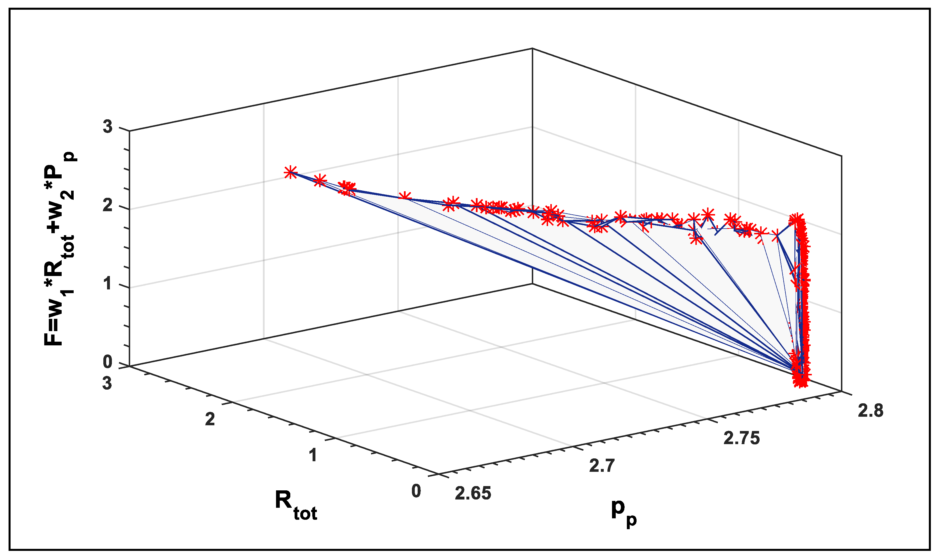
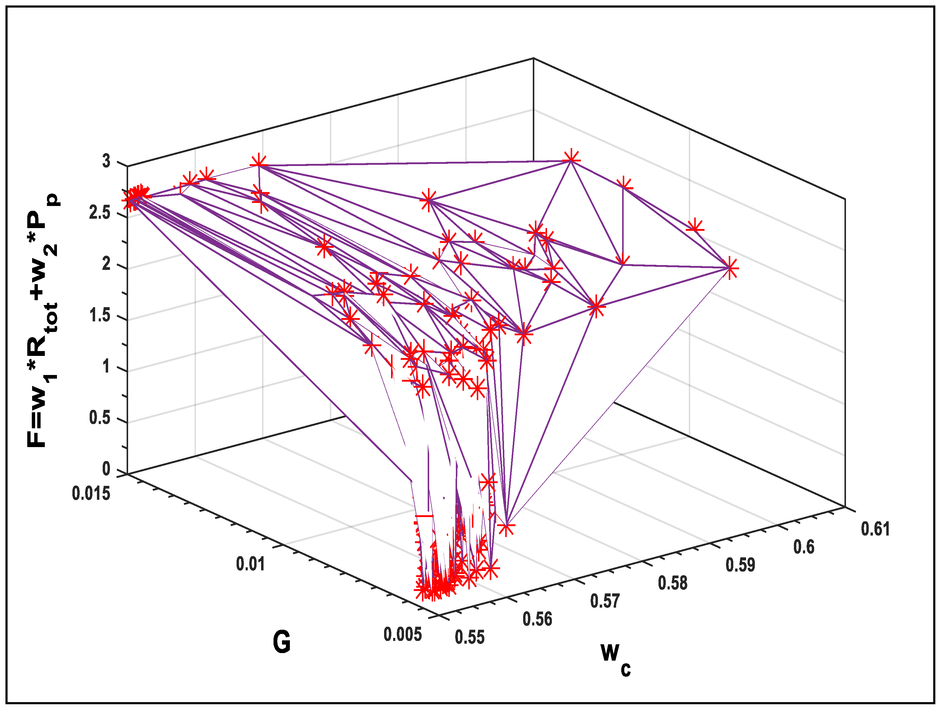
The aim of microchannel heat sink optimization is to minimize the multi-objective function regarding choosing the optimum values for the variables from the feasible region. It is a bi-objective optimization with objectives of optimizing thermal resistance and the pumping power. By having a different combination of weights, the weighting method has an advantage of obtaining multiple solutions from the Pareto front, when compared to classical methods like the ideal point method. Hence, a weighted approach for the objectives R_tot and P_p can be used as follows:

$$F=w_1{R}_{tot}+w_2{P}_P$$

(21)

With

$$w_1+w_2=1$$

where w₁ and w₂ are the weights associated with both performance parameters.

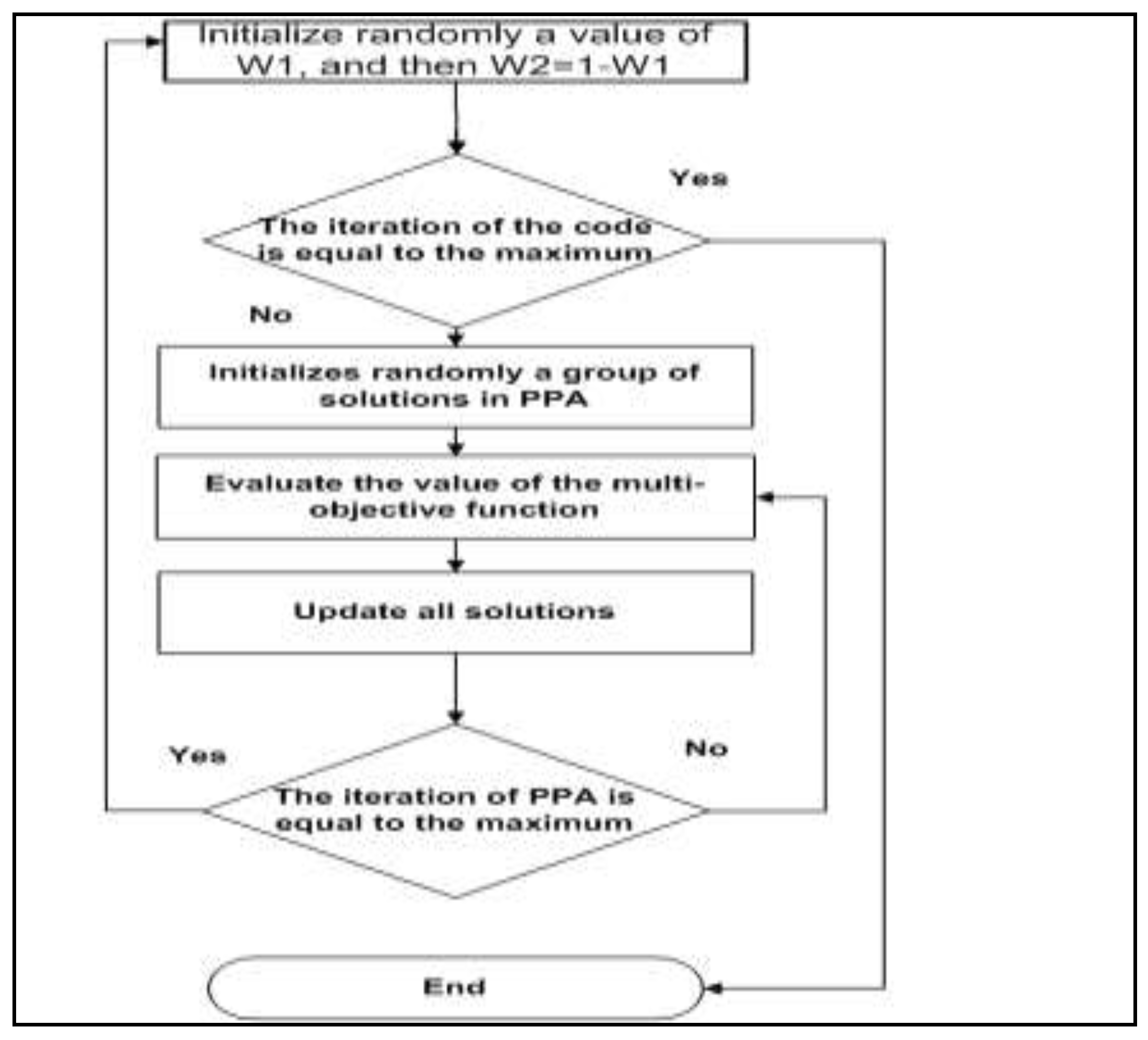
Even though assigning weights is subjective, and sometimes a challenging task for the decision-maker, a random or pseudo-random weight can be used to generate an approximate Pareto optimal solution that may well represent deferent corners of the Pareto front. If partial information can be accessed about the relationship on the weights, then by using that incomplete information pseudo-random weights can be generated and used. Otherwise, different weights can be generated randomly and utilized. After updating the weights, PPA is initialized with a population of random solutions and then upgraded through generations, as shown in Figure 4. The variables for both performance parameters are α and β.

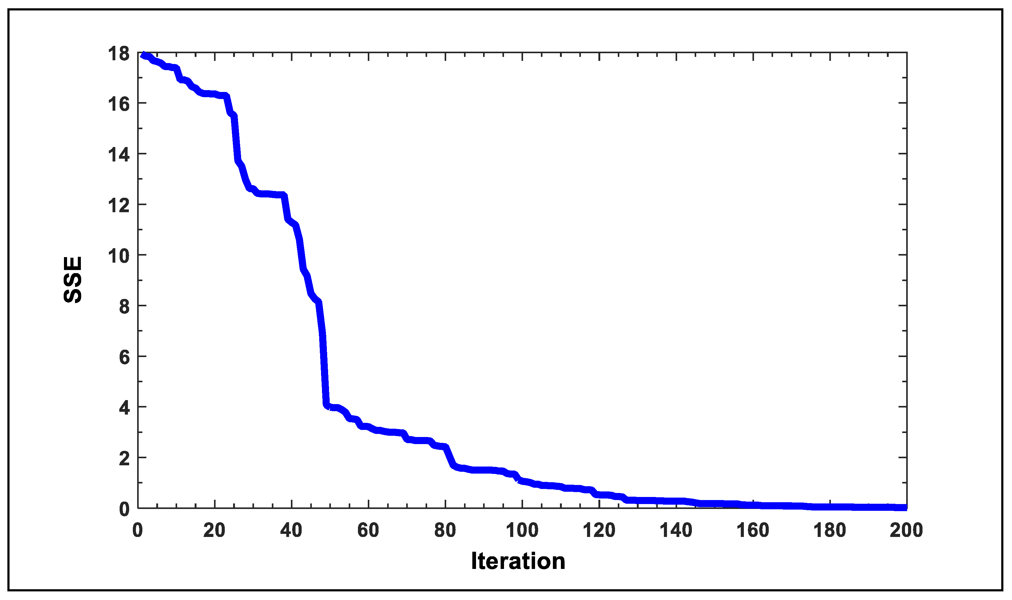
4.2. Radial Basis Function Neural Networks

RBFNNs typically have three layers: an input layer, a hidden layer with a non-linear activation function, and a linear output layer, as shown in Figure 5. The input layer is made up of source neurons that connect the network to its environment. The hidden layer receives the input information, followed by specific decomposition, extraction, and transformation steps to generate the output data. Additionally, the hidden layer’s neurons are associated with parameters (centers and widths), that determine the behavioral structure of the network. The neurons are linked together by parameters called the weights. The weights are divided into two types: the input weights and the output weights. The input weights are linked between the input layer and the hidden layer, and equal one for all. On the other hand, the output weights are linked between the hidden layer and the output layer, and all of them are variables. The output weights are calculated with the hidden layer parameters by using the optimization algorithms. In this paper, we have used PPA to determine the optimal values of the neural networks parameters. The output layer provides the response of the network to the activation pattern of the input layer that serves as a summation unit [54].

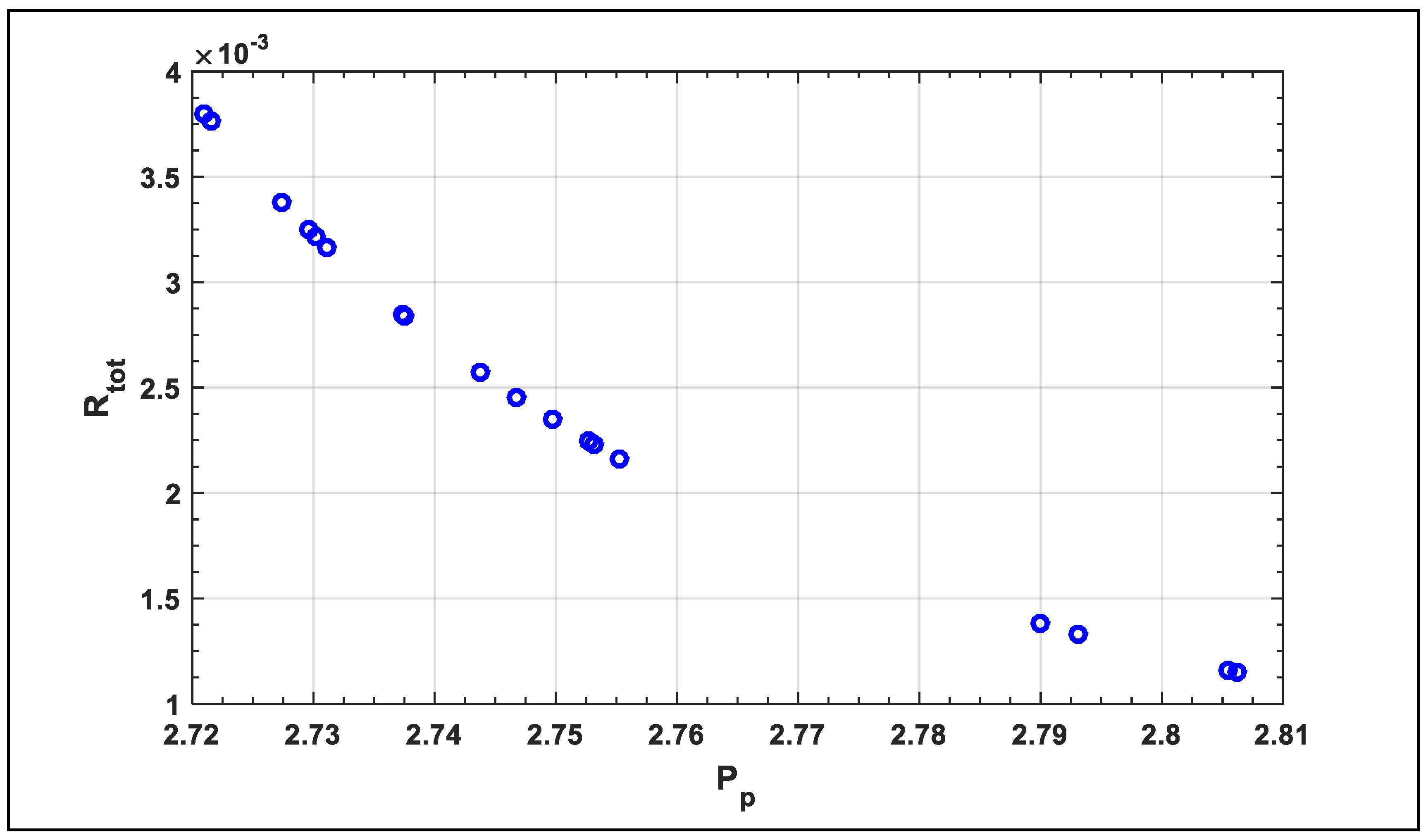
In this study, we used the RBFNNs to construct a model to represent the relationship between R_tot and P_p. In the proposed model, the input value is a P_p value, and the output is the corresponding R_tot value. The following equation is the Gaussian function (the activation function of the hidden neurons) that we use in RBFNNs [54]:

$${\phi }_i\left(x\right)=e^{-\left(\frac{{|x_i-{\mu }_i|}^2}{2{\sigma }_i{}^2}\right)}$$

(22)

where ${\phi }_i$ is the radial basis function in hidden neuron i, (x_i = ${\displaystyle \sum _{j=1}^N}{w}_{ji}^{\prime }\ast x_j$) is the input value in hidden neuron i, μ, and ${\sigma }_i^2$ are the center and the width of the hidden neuron i, respectively, N is the number of input neurons that are linked to hidden neuron i, $w_{ji}^{\prime }$ is the constant input weight from the input neuron j to the hidden neuron i which we fixed to be equal 1, and x_j is the input value in input neuron j.

Additionally, the actual values of the output layer can be determined using Equation (23):

$$F_K(x_i)={\displaystyle \sum }_{j=1}^M{w}_k^i{\phi }_j(x_i)$$

(23)

where F_k(x_i) is the actual output value of the output neuron k which corresponding to the input value x_i, $w_k^j$ is the output weight between the hidden neuron j and the output neuron k, and ${\phi }_j$ is the activation function in a hidden neuron j.

5. Results and Discussion

The simulation is performed using MATLAB R2015. The initial values for both w₁ and w₂ were taken randomly 300 times while the number of the iteration in PPA is set to 50, with the number of initial population of 50, the number of predators set to 5, the local search directions set to 8, and the number of best prey set to 12. Note that, increasing parameter values of PPA will increase the opportunity to obtain the best solution, but this will lead to a decrease of the algorithm speed. Therefore, choosing reasonable parameter values will satisfy the requirement.

As a result of our simulation, one of the final solutions is found to be P_p = 2.79344, R_tot = 0.134133 which correspond to the minimum value of the multi-objective function F = 0.138016, as shown in Figure 6, demonstrates the two objectives against the weighted sum of the goals. Ultimately, the solutions converge to the Pareto front as shown in Figure 7. The values, which correspond to the optimal solution, are shown in

Table 2. Parameter values of the optimization result.

Weight w1	Weight w2	wc	ww	G	N
0.99853	0.001462	0.68274	0.551488	0.00556	40.87455

.

As shown in Figure 6 and Figure 7, different corners of the Pareto front have been well approximated. A decision-maker can then look at the area based on the subjective judgment and make an informed decision. Moreover, Figure 6 and Figure 7 show that by increasing the value of P_p by decreasing the values of R_tot, then the optimal values of F is found. Figure 8 and Figure 9 show the response surfaces of F for the parameters w_w, and G with w_c, against the weighted sum of the objective functions, demonstrating the effectiveness of PPA in finding the optimal solutions. Decreasing the parameters has greater impact on estimating the optimal values of R_tot and P_p.

In addition, by using the PPA to train the neural network, the results which we found (using the parameters of the neural networks68 model) are shown in

Table 3. Neural network parameters.

Weights		Centers		Widths
ω1	1.08	μ1	3.83	σ1	1.48
ω2	3.99	μ2	1.28	σ2	3
ω3	3.99	μ3	1.36	σ3	1
ω4	1.11	μ4	2.76	σ4	1.01
ω5	3.78	μ5	4.5	σ5	2.65

, with the sum of squared error (SSE = 0.03709), as shown in Figure 10. This is performed with one input neuron, five hidden neurons, and one output neuron. PPA is used to optimize all parameters—output weights, the centers, and widths of the hidden neurons—to improve the performance of RBFNN.

We also used the analysis of variance (ANOVA) method to test the actual values of R_tot with its corresponding values with RBFNNs. ANOVA is a method for testing the hypothesis that the population means are equal. In ANOVA, a small p-value leads to rejection of the null hypothesis of equal means. A large p-value (such as greater than 0.001), fails to reject the null hypothesis of equal means [55]. Note that the F-test formula (Equation (24)) is used to determine the p-values [55]. In Equation (24), the $\mathrm{mean}\mathrm{square}(\mathrm{MS})$ represents the variation of variances between and within samples. For the single factor presented in

Table 4. Analysis of variance (ANOVA).

Source of Variation	SS	df	MS	F	p-Value	Critical Values
Between Groups	0.680727	1	0.680727	10.44468	0.001299	0.001
Within Groups	38.32258	588	0.065174	-	-	-
Total	39.00331	589	-	-	-	-

, the p-value (0.0013) is greater than the critical value (0.001), and this indicates that the model adequately predicts the experimental results.

$$F=\frac{\mathrm{Variance}\mathrm{between}\mathrm{sampels}}{\mathrm{Variance}\mathrm{within}\mathrm{sampels}}=\frac{\mathrm{MS}(\mathrm{between}\mathrm{sampels})}{\mathrm{MS}(\mathrm{within}\mathrm{sampels})}$$

(24)

6. Conclusions

The prey–predator algorithm was used to evaluate the best performance of the heat sinks. Thermal resistance and pressure drop networks were chosen as a multi-objective function. The performance within the prey–predator algorithm was found to be in good agreement with the Pareto front. The radial basis function neural network with the prey–predator algorithm was used successfully to predict the best performance of the microchannel heat sink. ANOVA statistical testing has shown that the neural networks are suitable for the prediction of the performance of the heat sinks.

References

1. Salman, B.; Mohammed, H.; Munisamy, K.; Kherbeet, A.S. Characteristics of heat transfer and fluid flow in microtube and microchannel using conventional fluids and nanofluids: A review. Renew. Sustain. Energy Rev. 2013, 28, 848–880. [Google Scholar] [CrossRef]
2. Jang, S.P.; Choi, S.U. Cooling performance of a microchannel heat sink with nanofluids. Appl. Therm. Eng. 2006, 26, 2457–2463. [Google Scholar] [CrossRef]
3. Chein, R.; Chen, J. Numerical study of the inlet/outlet arrangement effect on microchannel heat sink performance. Int. J. Therm. Sci. 2009, 48, 1627–1638. [Google Scholar] [CrossRef]
4. Gong, L.; Kota, K.; Tao, W.; Joshi, Y. Parametric numerical study of flow and heat transfer in microchannels with wavy walls. J. Heat Transf. 2011, 133, 051702. [Google Scholar] [CrossRef]
5. Tuckerman, D.B.; Pease, R.F.W. High-performance heat sinking for VLSI. IEEE Electron Device Lett. 1981, 2, 126–129. [Google Scholar] [CrossRef]
6. Zhang, C.; Lian, Y.; Yu, X.; Liu, W.; Teng, J.; Xu, T.; Hsu, C.-H.; Chang, Y.-J.; Greif, R. Numerical and experimental studies on laminar hydrodynamic and thermal characteristics in fractal-like microchannel networks. Part A: Comparisons of two numerical analysis methods on friction factor and Nusselt number. Int. J. Heat Mass Transf. 2013, 66, 930–938. [Google Scholar] [CrossRef]
7. Seyf, H.R.; Feizbakhshi, M. Computational analysis of nanofluid effects on convective heat transfer enhancement of micro-pin-fin heat sinks. Int. J. Therm. Sci. 2012, 58, 168–179. [Google Scholar] [CrossRef]
8. Rajabifar, B.; Seyf, H.R.; Zhang, Y.; Khanna, S.K. Flow and heat transfer in micro pin fin heat sinks with nano-encapsulated phase change materials. J. Heat Transf. 2016, 138, 062401. [Google Scholar] [CrossRef]
9. Seyf, H.R.; Zhou, Z.; Ma, H.; Zhang, Y. Three dimensional numerical study of heat-transfer enhancement by nano-encapsulated phase change material slurry in microtube heat sinks with tangential impingement. Int. J. Heat Mass Transf. 2013, 56, 561–573. [Google Scholar] [CrossRef]
10. Seyf, H.R.; Layeghi, M. Numerical analysis of convective heat transfer from an elliptic pin fin heat sink with and without metal foam insert. J. Heat Transf. 2010, 132, 071401. [Google Scholar] [CrossRef]
11. Short, B.E.; Raad, P.E.; Price, D.C. Performance of pin fin cast aluminum coldwalls, part 1: Friction factor correlations. J. Thermophys. Heat Transf. 2002, 16, 389–396. [Google Scholar] [CrossRef]
12. John, T.; Mathew, B.; Hegab, H. Parametric study on the combined thermal and hydraulic performance of single phase micro pin-fin heat sinks part I: Square and circle geometries. Int. J. Therm. Sci. 2010, 49, 2177–2190. [Google Scholar] [CrossRef]
13. Tullius, J.; Tullius, T.; Bayazitoglu, Y. Optimization of short micro pin fins in minichannels. Int. J. Heat Mass Transf. 2012, 55, 3921–3932. [Google Scholar] [CrossRef]
14. Adewumi, O.; Bello-Ochende, T.; Meyer, J.P. Constructal design of combined microchannel and micro pin fins for electronic cooling. Int. J. Heat Mass Transf. 2013, 66, 315–323. [Google Scholar] [CrossRef] [Green Version]
15. Abdoli, A.; Jimenez, G.; Dulikravich, G.S. Thermo-fluid analysis of micro pin-fin array cooling configurations for high heat fluxes with a hot spot. Int. J. Therm. Sci. 2015, 90, 290–297. [Google Scholar] [CrossRef]
16. Vanapalli, S.; ter Brake, H.J.; Jansen, H.V.; Burger, J.F.; Holland, H.J.; Veenstra, T.; Elwenspoek, M.C. Pressure drop of laminar gas flows in a microchannel containing various pillar matrices. J. Micromechan. Microeng. 2007, 17, 1381–1386. [Google Scholar] [CrossRef] [Green Version]
17. Tilahun, S.L.; Ong, H.C. Prey-predator algorithm: A new metaheuristic algorithm for optimization problems. Int. J. Inf. Technol. Decis. Mak. 2015, 14, 1331–1352. [Google Scholar] [CrossRef]
18. Hamadneh, N.; Khan, W.A.; Sathasivam, S.; Ong, H.C. Design optimization of pin fin geometry using particle swarm optimization algorithm. PLoS ONE 2013, 8, e66080. [Google Scholar] [CrossRef] [PubMed]
19. Hamadneh, N.; Tilahun, S.L.; Sathasivam, S.; Choon, O.H. Prey-predator algorithm as a new optimization technique using in radial basis function neural networks. Res. J. Appl. Sci. 2013, 8, 383–387. [Google Scholar]
20. Chou, J.-S.; Ngo, N.-T. Modified firefly algorithm for multidimensional optimization in structural design problems. Struct. Multidiscip. Optim. 2016, 1–16. [Google Scholar] [CrossRef]
21. Tilahun, S.L.; Ong, H.C. Bus timetabling as a fuzzy multiobjective optimization problem using preference-based genetic algorithm. Promet Traff. Transp. 2012, 24, 183–191. [Google Scholar] [CrossRef]
22. Khan, W.S.; Hamadneh, N.N.; Khan, W.A. Prediction of thermal conductivity of polyvinylpyrrolidone (PVP) electrospun nanocomposite fibers using artificial neural network and prey-predator algorithm. PLoS ONE 2017, 12, e0183920. [Google Scholar] [CrossRef] [PubMed]
23. Tilahun, S.L.; Goshu, N.N.; Ngnotchouye, J.M.T. Prey Predator Algorithm for Travelling Salesman Problem: Application on the Ethiopian Tourism Sites. In Handbook of Research on Holistic Optimization Techniques in the Hospitality, Tourism, and Travel Industry; IGI Global: Hershey, PA, USA, 2016; pp. 400–422. [Google Scholar]
24. Tilahun, S.L. Prey predator hyperheuristic. Appl. Soft Comput. 2017, 59, 104–114. [Google Scholar] [CrossRef]
25. Tilahun, S.L.; Ong, H.C.; Ngnotchouye, J.M.T. Extended Prey-Predator Algorithm with a Group Hunting Scenario. Adv. Oper. Res. 2016, 2016, 1–14. [Google Scholar] [CrossRef]
26. Tilahun, S.L.; Ngnotchouye, J.M.T.; Hamadneh, N.N. Continuous versions of firefly algorithm: A review. Artif. Intell. Rev. 2017, 1–48. [Google Scholar] [CrossRef]
27. Ong, H.C.; Tilahun, S.L.; Lee, W.S.; Ngnotchouye, J.M.T. Comparative Study of Prey Predator Algorithm and Firefly Algorithm. Intell. Autom. Soft Comput. 2017, 1–8. [Google Scholar] [CrossRef]
28. Lee, S.; Ha, J.; Zokhirova, M.; Moon, H.; Lee, J. Background Information of Deep Learning for Structural Engineering. Arch. Comput. Methods Eng. 2017, 25, 121–129. [Google Scholar] [CrossRef]
29. Adetiba, E.; Olugbara, O.O. Improved classification of lung cancer using radial basis function neural network with affine transforms of voss representation. PLoS ONE 2015, 10, e0143542. [Google Scholar] [CrossRef] [PubMed]
30. Hamadneh, N. Logic Programming in Radial Basis Function Neural Networks; Universiti Sains Malaysia: Penang, Malaysia, 2013. [Google Scholar]
31. Hamadneh, N.; Sathasivam, S.; Choon, O.H. Higher order logic programming in radial basis function neural network. Appl. Math. Sci. 2012, 6, 115–127. [Google Scholar]
32. Khan, W.A.; Yovanovich, M.; Culham, J.R. Optimization of microchannel heat sinks using entropy generation minimization method. IEEE Trans. Compon. Packag. Technol. 2009, 32, 243–251. [Google Scholar] [CrossRef]
33. Abbassi, H. Entropy generation analysis in a uniformly heated microchannel heat sink. Energy 2007, 32, 1932–1947. [Google Scholar] [CrossRef]
34. Adham, A.M.; Mohd-Ghazali, N.; Ahmad, R. Optimization of a rectangular microchannel heat sink using entropy generation minimization (EGM) and genetic algorithm (GA). Arab. J. Sci. Eng. 2014, 39, 7211–7222. [Google Scholar] [CrossRef]
35. Chen, K. Second-law analysis and optimization of microchannel flows subjected to different thermal boundary conditions. Int. J. Energy Res. 2005, 29, 249–263. [Google Scholar] [CrossRef]
36. Li, J.; Kleinstreuer, C. Entropy generation analysis for nanofluid flow in microchannels. J. Heat Transf. 2010, 132, 122401. [Google Scholar] [CrossRef]
37. Adham, A.M.; Mohd-Ghazali, N.; Ahmad, R. Thermal and hydrodynamic analysis of microchannel heat sinks: A review. Renew. Sustain. Energy Rev. 2013, 21, 614–622. [Google Scholar] [CrossRef]
38. Wang, Z.-H.; Wang, X.-D.; Yan, W.-M.; Duan, Y.-Y.; Lee, D.-J.; Xu, J.-L. Multi-parameters optimization for microchannel heat sink using inverse problem method. Int. J. Heat Mass Transf. 2011, 54, 2811–2819. [Google Scholar] [CrossRef]
39. Karathanassis, I.K.; Papanicolaou, E.; Belessiotis, V.; Bergeles, G.C. Multi-objective design optimization of a micro heat sink for Concentrating Photovoltaic/Thermal (CPVT) systems using a genetic algorithm. Appl. Therm. Eng. 2013, 59, 733–744. [Google Scholar] [CrossRef]
40. Ndao, S.; Peles, Y.; Jensen, M.K. Multi-objective thermal design optimization and comparative analysis of electronics cooling technologies. Int. J. Heat Mass Transf. 2009, 52, 4317–4326. [Google Scholar] [CrossRef]
41. Normah, G.-M.; Oh, J.-T.; Chien, N.B.; Choi, K.-I.; Robiah, A. Comparison of the optimized thermal performance of square and circular ammonia-cooled microchannel heat sink with genetic algorithm. Energy Convers. Manag. 2015, 102, 59–65. [Google Scholar] [CrossRef]
42. Khan, W.A.; Kadri, M.B.; Ali, Q. Optimization of microchannel heat sinks using genetic algorithm. Heat Transf. Eng. 2013, 34, 279–287. [Google Scholar] [CrossRef]
43. Shao, B.; Sun, Z.; Wang, L. Optimization design of microchannel cooling heat sink. Int. J. Numer. Methods Heat Fluid Flow 2007, 17, 628–637. [Google Scholar] [CrossRef]
44. Shao, B.; Wang, L.; Cheng, H.; Li, J. Optimization and numerical simulation of multi-layer microchannel heat sink. Procedia Eng. 2012, 31, 928–933. [Google Scholar] [CrossRef]
45. Knight, R.W.; Hall, D.J.; Goodling, J.S.; Jaeger, R.C. Heat sink optimization with application to microchannels. IEEE Trans. Compon. Hybrids Manuf. Technol. 1992, 15, 832–842. [Google Scholar] [CrossRef]
46. Hu, G.; Xu, S. Optimization design of microchannel heat sink based on SQP method and numerical simulation. In Proceedings of the 2009 IEEE International Conference on Applied Superconductivity and Electromagnetic Devices (ASEMD 2009), Chengdu, China, 25–27 September 2009; pp. 89–92. [Google Scholar]
47. Dede, E.M. Optimization and design of a multipass branching microchannel heat sink for electronics cooling. J. Electron. Packag. 2012, 134, 041001. [Google Scholar] [CrossRef]
48. Husain, A.; Kim, K.-Y. Shape optimization of micro-channel heat sink for micro-electronic cooling. IEEE Trans. Compon. Packag. Technol. 2008, 31, 322–330. [Google Scholar] [CrossRef]
49. Kou, H.-S.; Lee, J.-J.; Chen, C.-W. Optimum thermal performance of microchannel heat sink by adjusting channel width and height. Int. Commun. Heat Mass Transf. 2008, 35, 577–582. [Google Scholar] [CrossRef]
50. Kleiner, M.B.; Kuhn, S.; Haberger, K. High performance forced air cooling scheme employing microchannel heat exchangers. IEEE Trans. Compon. Packag. Manuf. Technol. Part A 1995, 18, 795–804. [Google Scholar] [CrossRef]
51. Cruz-Duarte, J.M.; Garcia-Perez, A.; Amaya-Contreras, I.M.; Correa-Cely, C.R. Designing a microchannel heat sink with colloidal coolants through the entropy generation minimisation criterion and global optimisation algorithms. Appl. Therm. Eng. 2016, 100, 1052–1062. [Google Scholar] [CrossRef]
52. Kim, S.; Kim, D. Forced convection in microstructures for electronic equipment cooling. J. Heat Transf. 1999, 121, 639–645. [Google Scholar] [CrossRef]
53. Phillips, R.J. Advances in Thermal Modeling of Electronic Components and Systems; ASME: New York, NY, USA, 1990; pp. 109–184. [Google Scholar]
54. Hamadneh, N.; Sathasivam, S.; Tilahun, S.L.; Choon, O.H. Learning logic programming in radial basis function network via genetic algorithm. J. Appl. Sci. 2012, 12, 840–847. [Google Scholar] [CrossRef]
55. Triola, M.F. Elementary Statistics; Pearson/Addison-Wesley: Reading, MA, USA, 2006. [Google Scholar]
Figure 1. Geometry of the microchannel heat sink.
Machines 06 00026 g001
Figure 2. Thermal resistance network.
Machines 06 00026 g002
Figure 3. Pressure drop network.
Machines 06 00026 g003
Figure 4. The flowchart for the optimization procedure.
Machines 06 00026 g004
Figure 5. Structure of a radial basis function neural network.
Machines 06 00026 g005
Figure 6. Relation between Rtot, Pp, and F.
Machines 06 00026 g006
Figure 7. Relation between Rtot and Pp.
Machines 06 00026 g007
Figure 8. Effect of ww and wc on F.
Machines 06 00026 g008
Figure 9. Effect of G and wc on F.
Machines 06 00026 g009
Figure 10. Performance of RBFNN based on PPA in terms of SSE.
Machines 06 00026 g010