Customized Knowledge Discovery in Databases methodology for the Control of Assembly Systems

Abstract

The advent of Industry 4.0 has brought to extremely powerful data collection possibilities. Despite this, the potential contained in databases is often partially exploited, especially focusing on the manufacturing field. There are several root causes of this paradox, but the crucial one is the absence of a well-established and standardized Industrial Big Data Analytics procedure, in particular for the application within the assembly systems. This work aims to develop a customized Knowledge Discovery in Databases (KDD) procedure for its application within the assembly department of Bosch VHIT S.p.A., active in the automotive industry. The work is focused on the data mining phase of the KDD process, where ARIMA method is used. Various applications to different lines of the assembly systems show the effectiveness of the customized KDD for the exploitation of production databases for the company, and for the spread of such a methodology to other companies too.

1. Introduction

The presence of powerful control alarm and clever decision systems is nowadays a critical element for the efficiency of manufacturing plants: reduction of unplanned issues and production stops is mandatory to keep up with competitors and to increase flexibility. In particular, manufacturers are aiming to move from corrective to preventive and, finally, to predictive and smart actions. Thanks to the evolved monitoring and electromechanical systems, such as Distributed Control Systems (DCS), Supervisory Control and Data Acquisition (SCADA), Micro Electro Mechanical Systems (MEMS) and Radio Frequency Identification (RFID), the implementation of predictive actions is continuously growing and both technical and economic constraints are gradually decreasing [1]. An entire branch of engineering, alarm management, is devoted to ensuring the effectiveness of this kind of tools [2]. A strong pulse in the development of alarm systems was given by the advent of Industry 4.0 (I4.0) and Cyber-Physical Systems (CPS), which are the main factors responsible for the contemporary evolution of classical manufacturing systems into digital ecosystems. In particular, the CPS is responsible for the fusion between the physical world and abstract knowledge, such as management, optimization, control and data processing. In this sense real and virtual systems are connected by means of data, which are then transformed into information and eventually into knowledge, to be able to take support management decisions [3]. While CPSs exist in common human daily life (for example, car sharing), Industrial CPS (ICPS) have special focus on novel approaches to system monitoring, fault diagnosis and control, aiming at achieving plant-wide intelligent manufacturing [4].

The major role in collecting and processing data is played by Internet of Things (IoT) and Big Data Analytics, on which both academic and business communities are spending a considering effort. IoT identifies a network of objects, interconnected through embedded technology to create a smart environment. In particular, Industrial Internet of Things (IIoT) implies the use of sensors, actuators, control systems, data analytics and security mechanisms. This continuous strengthening in interconnection capabilities leads to the generation and the collection of large volumes of data. These data, which by 2020 will be over 40 trillion gigabytes, are generally called Industrial Big Data [5]. IIoT and Big Data Analytics can allow better control and management of production systems. Data analytics aims at analyzing raw data to extract useful information and transfer it to effective knowledge, to improve process understanding and to support decisions [6]. In particular, the exploitation of Big Data through analytics in manufacturing industries can decrease product development and assembly costs by up to 50% and can cause a 7% reduction in the working capital [7]. Moreover, the strategical and commercial potential minable from IIoT can be quantified in billions of dollars [8].

Actually, Big Data Analytics procedures appear as far away from being implemented on a full-scale range inside manufacturing plants. This situation can be seen as a counter-productive paradox, since the economic and technical effort required to install I4.0 systems is not justified by the obtained gain, and it could provide motivations for investigating in this direction. The concept is highlighted in Figure 1, representing the outcome of academic research on Big Data usage in the timespan 2010–2016, in which manufacturing accounts only for 8% [9].

The main reasons explaining this phenomenon are:

• Poverty of well-defined and standardized data analysis procedures and guidelines for manufacturing datasets [8];
• Absence of a consolidated data analysis culture in the manufacturing field [9];
• Scarcity of well-established and appropriate data collection and saving systems; and
• Issues with data accessibility and sharing.

These pitfalls are exposing companies to a not full understanding of how they could really exploit the hidden knowledge present in their databases to improve their performance and so their competitiveness on the market. Especially, the implementation of a correct Big Data Analytics procedure is found to be fragile in the context of assembly systems, where very poor machine data are available.

The contributions of this work are as follows. Firstly, the Knowledge Discovery in Databases (KDD) methodology is suitably customized for the context of process engineering and assembly systems. Each step of this architecture is discussed in details to underline nature of available data, targets of proposed methodology and novel points with respect to traditional KDD procedures [10]. Secondly, within the development of the KDD steps, the definition and implementation of a personalized Autoregressive Integrated Moving Average (ARIMA) are built to analyze products data and predict any unforeseen issue within the assembly stations.

The remainder of the paper is structured as follows. Section 2 explains the need to investigate deeper how it is possible to analyze industrial assembly systems databases through a systematic methodology, which is presented in Section 3. The aim is to gain knowledge from processes within Bosch VHIT S.p.A., active in the sector of the automotive industry worldwide, also presented in Section 3. Section 4 deeply describes the adopted KDD-based methodology. Since the Data Mining stage results to be the most critical KDD step, Section 5 is specifically devoted to it, explaining the development of a personalized Autoregressive Integrated Moving Average (ARIMA) model and the criteria adopted to choose it with respect to alternative solutions. Section 6 shows results achievable by the KDD-ARIMA application to the considered industrial case, highlighting the added value concretely achievable by the company in terms of time and money saved. Finally, Section 7 supplies main conclusions of the work from both academic and practitioner perspectives. Some tips for possible future works and extensions are presented, too.

2. Research Statement and Objective

Considering the manufacturing systems as made by two main subsets, machining and assembly systems, the second one appears as the weakest one from the point of view of real time data exploitation and development of models for predictive actions, as highlighted through literature research [11,12,13,14,15]. This is mainly due to the nature of the process: machining is featured by a critical state of stress between workpiece and tool and by the consequent presence of a systematic wear mechanism in between them. On the other hand, assembly tools can work for extremely long periods because of the absence of comparable stresses and failures are mainly due to peculiar and non-repeatable phenomena. Entering into the details, next points highlight why several tools, being powerful and effective in case of repeatable issues, typical of machining department, fail when moving to a more uncertain scenario, typical of assembly one:

• Assembly datasets mainly focus on quality variables and process parameters, leading to the generation of discrete time series related to processed items instead of continuous signals coming from equipment. Therefore, the nature of available data, as deeply discussed in Section 3.2, prevents the creation of models based on signals coming from sensors and describing machines technical parameters such as temperatures, absorbed powers or vibrations. This concept explains why powerful and reliable techniques provided by ICPS, such as data-driven KPI estimators and predictors, based on real or soft sensors [4], are not completely applicable to this specific context.
• Techniques typical of the control theory [16,17], such as dynamic state space models or observers (e.g., Kalman filter), could not be used because the tracking of different and multiple issues, featured by different physical reasons, could not be reliable in case of single mathematical modeling. Moreover, even if these strategies would be able to identify a certain deviation with respect to the typical stable scenario, they are not able to identify the root cause of the problem, leading to a partial effectiveness of predictive action.

Despite these issues, it is clear that large datasets are actually available on assembly systems, too. Mainly, because assembly is the very last processing phase of production and the only point in which it is possible to test a product’s compliant functioning before its shipping, the availability of production data during this processing stage is crucial for quality monitoring and product’s traceability, in case of future issues with customers. Considering this aspect, the construction of databases in assembly environments becomes almost mandatory and each analysis tool focused on them could result in real added value for the company adopting it.

Research Objective

Considering the explained constraints, the presented work aims to apply an effective methodology to describe the appearance of any issue, not depending on the physical root cause, and to allow the development of a predictive tool in the assembly systems. To fulfill this target, a well-known methodology for Big Data analysis, the Knowledge Discovery in Databases (KDD), has been customized. In particular, Data Mining stage of KDD will be faced adopting the ARIMA algorithm, specifically tuned for the considered application.

X_t = ϕ₁X_t−1 + ⋯ + ϕ_pX_t−p + Z_t − ϑ₁Z_t−1 − … − ϑ_qZ_t−q

(1)

The ARIMA model, presented in Equation (1), is fitted on time series data both to better understand the data themselves and predict future points in the series. ARIMA model is applied where data show evidence of non-stationarity, allowing to capture sudden deviations in a generally planar data sequence [18].

The methodology is applied and validated within Bosch VHIT S.p.A. In so doing, the analyst could quickly identify the optimal path and extract tangible information from available raw data. Some cornerstones driving the customization of KDD will be:

• Consistency. Each step will be motivated and justified from both a mathematical-analytical and a physical-industrial point of view.
• Generality. Even though the tool will be specifically designed and validated within the Bosch VHIT S.p.A. assembly system, it strives for being a standardized instrument, applicable by a manufacturing industry independently from nature and layout of performed assembly process. Moreover, it aims to be easily tunable and customizable, depending on the local field of application, so to optimize its performances for the specific case study.

Before proceeding with the development of the customized KDD, Section 3 recalls basic concepts about KDD, with the purpose to sustain the choice of adopting this methodology. Then, the Bosch VHIT S.p.A. assembly system is described, to define the scope of the work the authors are dealing with.

3. Background

3.1. KDD Methodology

KDD is one of the most popular and consolidated methodologies concerning Big Data Analysis. It started to be widely investigated and discussed in the late 1990s [19]. Essentially, it is the process of discovering useful knowledge from a raw collection of data, through the application of exploratory algorithms. Typically, knowledge is intended as the recognition of hidden patterns and their exploitation to provide novel benefits to the user [20]. Since data size is enormous and information can be an extremely smaller portion of them, it is impossible to manually highlight knowledge or significant patterns. There are three main motivations in favor of KDD application:

• Capability to reduce Big Data original size, decreasing computational cost and associated technical problems, by focusing on useful variables only.
• Capability to work in uncertain situations. Since the goal of KDD is to extract knowledge from raw data, it is naturally built to be flexible and to adapt its framework with respect to partial results obtained along its application.
• Popularity and generality. Academic literature suggests KDD as the most suitable methodology to be used for the sake of information extraction from raw Big Data [21,22]. The main reason is that it gives very general guidelines, leaving to the practitioner a sufficient number of degrees of freedom to develop and adapt it to the actual case.

The logical structure of a KDD process is depicted in Figure 2, and is made by five main steps to be performed by the analyst [23,24,25,26,27]. This framework has a complex iterative nature, with loops rising at different layers and resulting in a nested architecture, which allows a continuous optimization and adaptation of the achievable performances. On the other hand, it could result to be too dispersive and, if well-defined criteria for algorithms’ selection and possible goals are not present, it could lead to two dangerous consequences. The first one is the random application of all available data analysis techniques, which could be extremely time-consuming, considering the high computational cost associated with Big Data. The second one is the convergence to a local optimum solution, driven again by the unjustified selection of data analysis algorithms or by missed preliminary considerations. Thus, the proper realization of each step is crucial not only for the convergence to a satisfying solution, but also to reduce the effort consumed in next passages.

3.2. Bosch VHIT S.p.A. Assembly System

Bosch VHIT S.p.A., in the following also addressed to as the company, is active in the automotive sector, focusing on the production of vacuum pumps, oil pumps, diesel pumps, combined pumps and hydro-boosters. Company assembly area is characterized by 19 lines equipped with real-time data collection and storage systems. The flow of data from assembly lines to databases, coupled with the absence of real-time data processing and analysis supplies the best conditions for the application of the proposed procedure since it represents a good example of partial exploitation of available gathered data at the shop-floor. (Figure 3). It should be noticed how the absence of a real-time data processing and analysis system precludes the generation of tangible added value for the enterprise, in terms of predictive actions.

Collected Data

To correctly apply and customize the KDD methodology, nature of available data must be clarified to understand why the company decided to collect them, to explain analysis strategy adopted in the rest of the work and to justify the targets of the analysis itself. The company has developed process databases in the format of tables, collecting the following information (either qualitative either categorical):

• General assembly layout information: codes for items’ traceability and model recognition, in case of multi-product lines; date and time of product processing; cycle time of each workstation.
• Single workstation information: physical variables referred to performed operation; station outcome (compliant or non-compliant piece).

These types of data are named structured data and are arranged in ordered manner, such as table and spreadsheets, in contrast with unstructured data, such as pictures, video and audio [28].

More in detail, within the assembly department, the process datasets collect all process parameters. The goal of process parameters, e.g. torques in tightening operations and forces during pressing, is to monitor product compliance in terms of customer’s quality requests. Currently, a product, passing through a certain workstation, is considered compliant if its process parameters lie inside an admissible range. Therefore, the collected variables are referred to products and not to machines. Each row of the dataset table reports data of a single processed item, especially for quality and traceability purposes in case of customers’ claims. This peculiarity of the data involves that typical predictive algorithms, based on signals from equipment describing health status rather than product information, are not perfectly aligned with the described situation and goals.

Thus, the available dataset allows pursuing the development of a customized KDD methodology for a twofold objective: first, to detect failures, possibly but not necessarily related to assembly equipment, to improve maintenance performance; and, secondly, to monitor and track quality performance of the realized products, even before the end-of-line compliance tests.

Without loss of generalization and scalability of the proposed data analytics methodology, this study focuses on the single workstation within an assembly line. In particular, the behavior of physical variables could be modeled to perform useful predictions to anticipate any unforeseen issue. This choice was agreed with company engineers and technicians, whose expertise suggest concentrating attention on critical variables paths, instead of searching for relationships between them. This explains why small effort has been concentrated on another fundamental aspect linked to ICPS: Multivariate Analysis (MVA) [4]. Again, powerful KPI estimation and fault prediction techniques, such as the Total Principle Component Regression (TPCR) [3], appear not suitable for the explained case study.

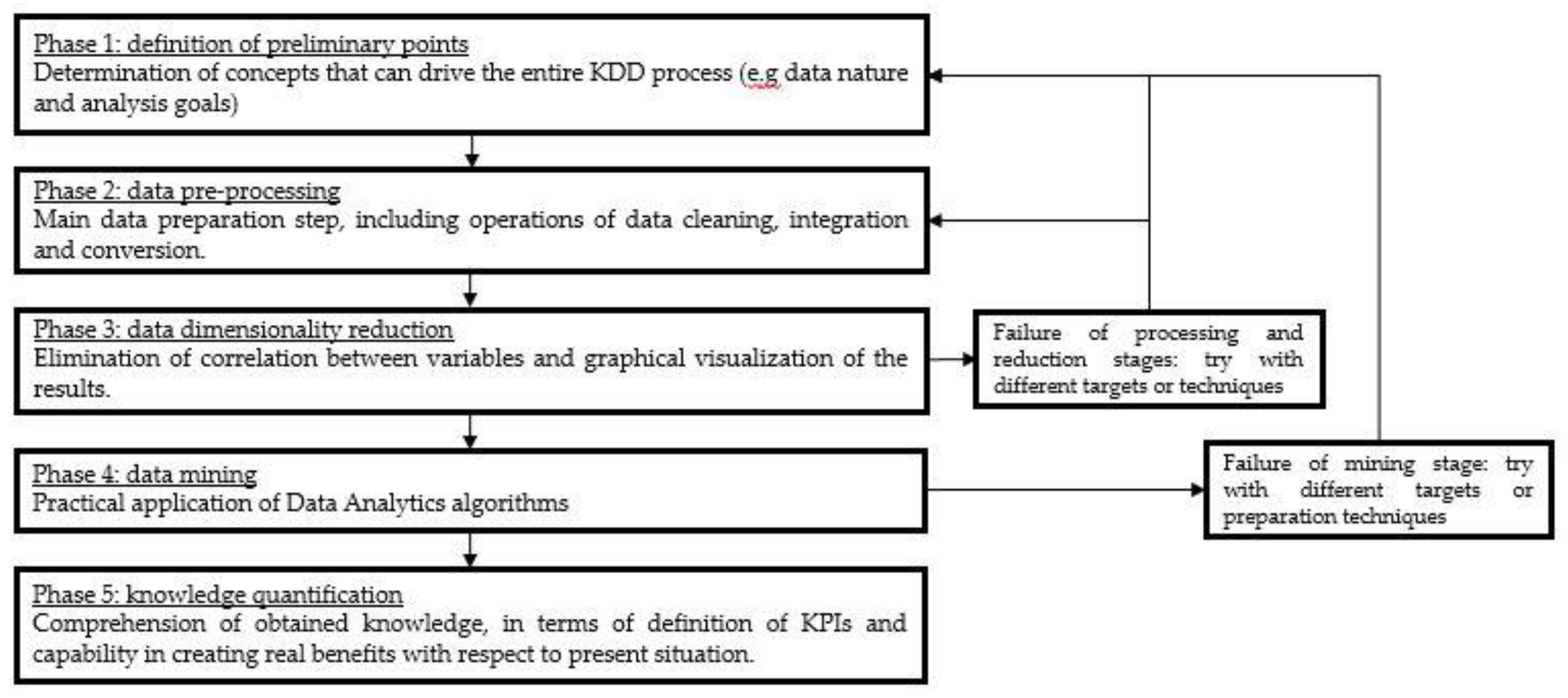
4. Customized KDD for Assembly System

The description of the customized KDD methodology for the company assembly system is carried out considering the KDD structure proposed in Figure 2 as backbone. In the next sections, each step is recalled and described to highlight any peculiarities with respect to the application of the KDD to the industrial case, i.e. the assembly system, and proposed improvements.

4.1. Definition of Preliminary Points

Fundamental preliminary points are determined in this first stage to learn next steps and to minimize useless future efforts. In particular, determination of data nature and possible goals have already been faced in Section 3.2.1: Structured datasets collecting process parameters to determine compliance of final products. Data nature deals with process parameters while analysis goal is about the development of a smart predictive tool. These cornerstones will drive all next passages.

4.2. Data Pre-processing

Data pre-processing is driven not only by analytic methods but also by common sense statements, derived after a first look at the examined dataset. Company assembly raw data are collected in rectangular tables, as usual for assembly systems [29]. It can be seen as a matrix X, having size n x p, as the one depicted in Equation (2). The generic cell xⁱ_j, with i = 1, … , n and j = 1, …, p, contains the value of the j-th parameter (variable) for the ith piece (item).

$$X=\left[\begin{array}{ccccc}{x}_1^1& \cdots & \cdots & \cdots & x_1^p\\ ⋮& ⋮& ⋮& ⋮& ⋮\\ x_i^1& \cdots & x_i^j& \cdots & x_i^p\\ ⋮& ⋮& ⋮& ⋮& ⋮\\ x_n^1& \cdots & \cdots & \cdots & x_n^p\end{array}\right]$$

(2)

Considering the analysis target, attention is focused on each single column of the database (namely, on each single physical variable measured in the considered workstation). The performed basic operations can be summarized by the next points:

• Position data in a chronological order. These operations help future time-series analysis and forecasting activities.
• Consider the proper period only. The whole available history is not always the best choice, even though it may bring to a better validation of used stochastics models. For example, immediately after the assembly line installation, the series production will start only after properly equipment regulation and prototyped products, thus gathered data are highly affected by this extraordinary situation.
• Eliminate outliers. An outlier is defined as a measurement that results inconsistent with respect to the rest of the dataset. Its value can be generated by different causes such as poorly calibrated or faulty instruments, electrical issues, communication channels issues, and server issues. The management of outliers is particularly puzzling since outliers considered as normal measurements can contaminate data behavior, compromising the identification of patterns and the algorithms’ functioning; however, normal measurements considered as outliers can obstruct the capture of useful knowledge. If one removes them, a fundamental portion of the dataset is going to be removed, namely the non-compliant pieces. Since the final goal is to prevent issues, based on past knowledge, the exclusion of these values from the database seems inappropriate. To verify that data are not real outliers, a check if a candidate outlier corresponds to a compliant piece must be performed: if the answer is positive, the measurement is inconsistent and the point is discarded; if the answer is negative, it is not possible to neglect the point. Then, it is important to understand how to manage value of these points, which is completely different from the remaining portion of the dataset. Since the difference can be of several orders of magnitude too, a single anomaly can affect the entire dataset behavior and compromise prediction and regression analysis. Thus, their value is shifted to positions that lie immediately outside the admissible range to include these values in the analysis while keeping their original information (i.e. the piece is not compliant).

4.3. Data Dimensionality Reduction

Data dimensionality reduction is used to eliminate correlation and to allow graphical representation of a multivariate dataset. In the considered situation, since analyst effort is focused on single variables and there is no research for relationships between different process parameters, this step is not necessary and data preparation could be considered solved with considerations in Section 4.2.

4.4. Data Mining

The data mining step can be considered as the main stage of the whole KDD process. Actually, it has to be divided into two subsections: selection and application of the algorithm. Target of the first stage is to provide a specific criterion so that the user can be oriented in the selection of most proper algorithms. An iterative procedure is suggested to exploit the partial knowledge learned until that moment and to cut the selection of possible algorithms after each step, converging to a satisfying solution. Target of second stage is the practical application of the chosen algorithm and the quantification of its results, to test the suitability of the selected algorithms or go for other alternatives.

The next subsection describes the developed algorithm’s selection criteria, while the data mining application is presented in Section 5 since the authors highly customize this mainstage of the KDD to make it more adherent with the scope of the work, i.e. assembly systems.

4.5. Development of Algorithm’s Selection Criteria

According to information collected from previous steps, algorithms coming from the world of statistical learning appear as the most appropriate ones to act on the considered datasets. Statistical learning is the set of tools used to understand data [30]. The application of algorithms proposed by this field of statistical science allows solving issues of pattern recognition and searching for association rules in between different variables. Since statistical learning techniques are various and copious, it is suggested to develop some selection criteria before starting with the actual data analysis stage. In particular, this research study proposes a selection procedure based on two selection layers to make the algorithm’s choice reliable. Firstly, algorithms are screened as a function of the mathematical nature of the problem and the expected goal. Secondly, a further selection based on the physics of the analyzed system is performed.

More in the details:

• Selection layer one deals with the mathematical nature of the problem. When referring to statistical learning literature, two main objectives are usually faced: inference problems, which involve the research of relationships between different variables and the subdivision of individuals in specific categories basing on the values of parameters describing them; prediction problems, which involve the modeling of variables and the attempt of forecasting their future behavior [31]. First kind of problem should be faced with classification techniques while second one with regression algorithms. According to proposed analysis goal, focused on single process parameters, it is clear that the actual analysis should find a solution of a prediction problem.
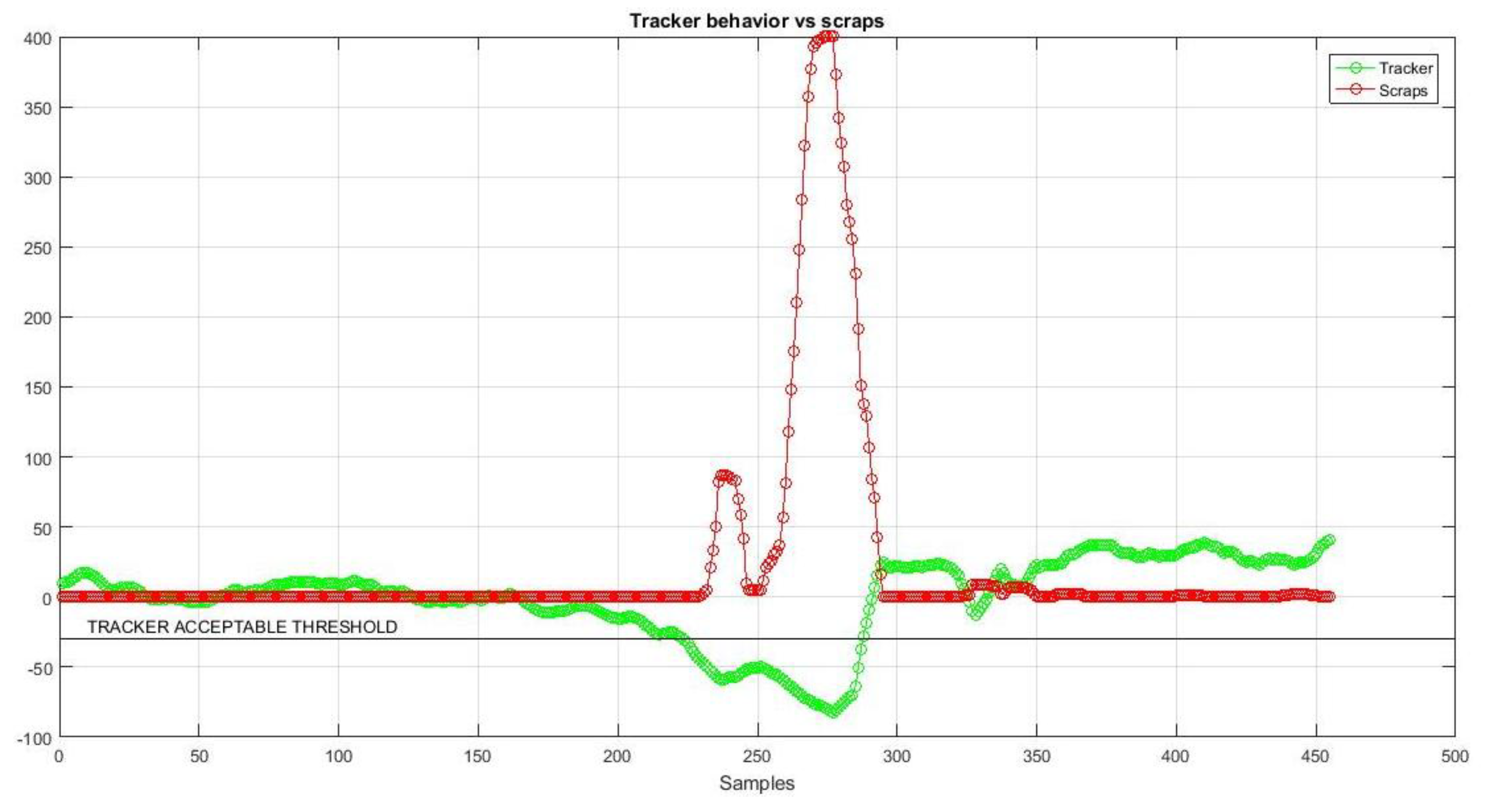
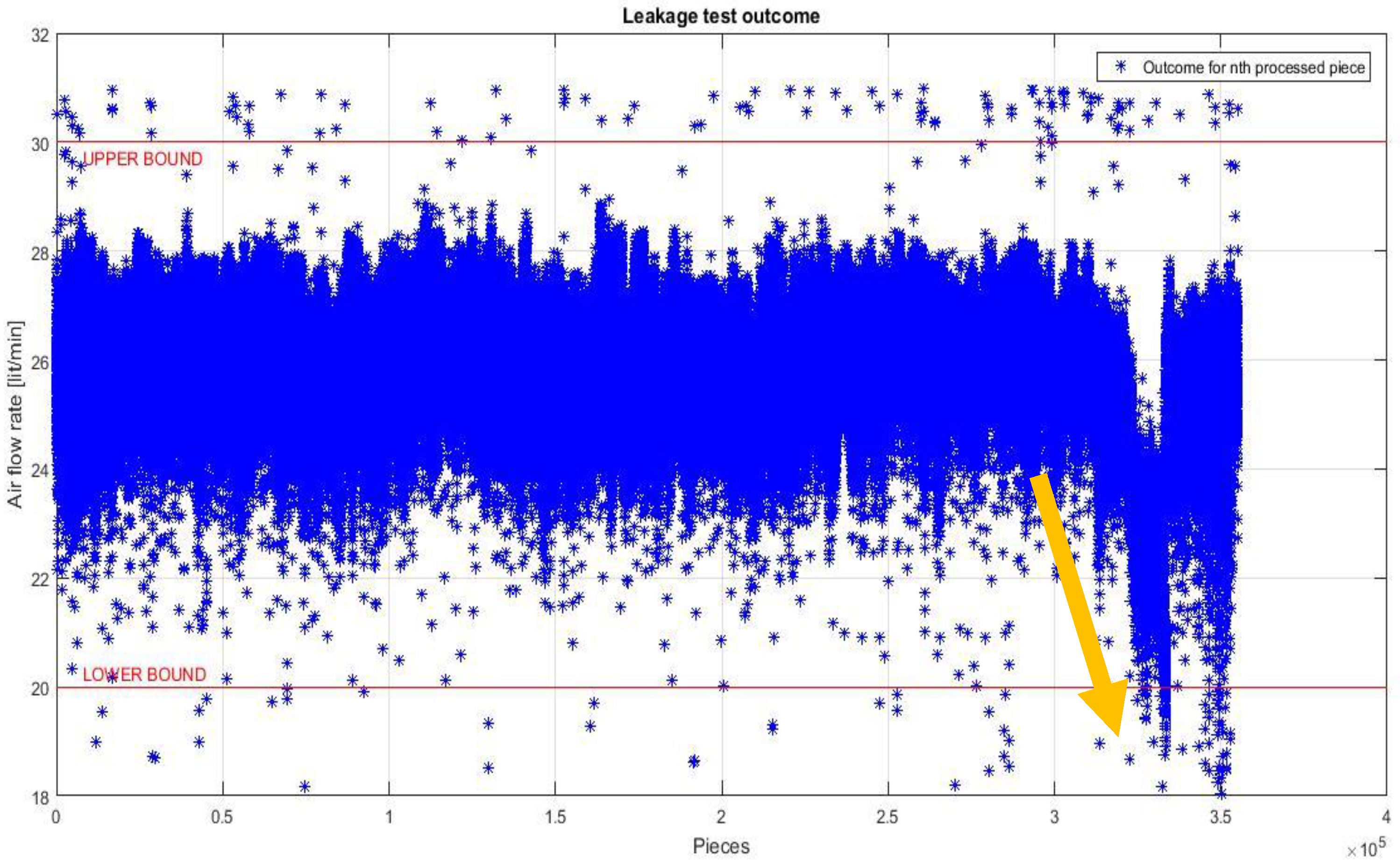
• Selection layer two deals with physical nature of the assembly system. Considering the very peculiar behavior of assembly systems, with the generation of almost non-repeatable technical or qualitative issues on different subgroups, data appear with a very particular shape. Process parameters sequences come with a general stable and planar behavior, spaced by local and isolated peaks caused by unique reasons. Each issue appears as an anomaly, namely a point in time where the behavior of the system is unusual and significantly different from previous and normal behavior. Figure 4, related to the time series of a process parameter collected in Bosch VHIT S.p.A., clearly shows this kind of behavior (see the area pointed by the arrow, highlighting the emerging behavior after 3,100,000 pieces).

The peculiar shape assumed by considered dataset suggests applying the group of statistical learning techniques belonging to novelty detection, which aims at recognizing data that differ somehow with respect to the ones collected during training stage [32]. The specific application of novelty detection techniques in industrial failure investigation is underlined by the literature [33]. Novelty detection allows identifying normal operating condition/s. When this normal threshold is passed, the system is showing a novel situation. Novelty detection should not be confused with outlier detection. Outliers are inconsistent with the rest of the dataset and they should be eliminated, as already stated in Section 4.2. Novelties are data points showing a new and never seen behavior, in our case strictly related to non-compliant pieces. The literature proposes a classification of novelty detection techniques in five main categories, depending on the nature of considered problem. In case of prediction, it is suggested to adopt novelty detection algorithms coming from “probabilistic approach” category [32].

Summarizing, an algorithm able to perform powerful predictions on assembly process parameters should be featured by a regression nature (mathematical selection stage) and by the capability of capturing sudden deviations in a generally planar data sequence (physical selection stage). An interesting candidate is the Autoregressive Integrated Moving Average (ARIMA) model, which is part of the “probabilistic approach” category of novelty detection techniques [18]. The reasons are basically two. Firstly, the high forecasting performances achievable by this method. Secondly, the innovative application of this algorithm, coming from financial and banking environments, to the manufacturing world.

5. Data Mining via ARIMA Modeling

ARIMA modeling technique derives from the economic world, but it has been found to be applicable and effective also in the industrial sector, especially for predictive maintenance and faults’ forecasting [34]. The idea is to investigate its performance when focusing on an assembly process, with its own particular features, especially the non-repeatability processes. Thus, the main feature of the model would be the adaptability to all possible problems affecting considered manufacturing environment, not depending on their physical nature. The capability to capture both technical and qualitative problems should be considered crucial exactly as the effectiveness of the future forecast with ARIMA modeling. For this reason, the application of this model to the considered case is divided in two macro portions: time series processing and ARIMA modeling.

In the first phase, the raw time series of the analyzed variable should somehow be processed (e.g., smoothened) to find a shape able to minimize fluctuations in case of nominal behavior of the system and to highlight every anomaly rising, not depending on its nature and on its growing rate. During second phase, the ARIMA model is applied to this series, trying to fit it in the best way so to optimize forecasting performances. Since a time series is defined as a collection of measurements taken with a fixed timespan, the time interval in between two consecutive points is considered equal to workstation cycle time.

To properly fulfill the goals of adaptability and generality, the model has been constructed thinking in a parametric way. Consequently, modeling is flanked by the definition of a tuning procedure for the parameters themselves. On the one hand, the tuning procedure should be systematic and automated enough to allow an easy and fast implementation of all interesting variables. On the other hand, it should leave some degrees of freedom to allow the best customization, and consequent optimization, with respect to the considered workstation. In order to better organize the model construction and to find the best trade-off between the previous needs, two types of parameters have been taken into account, as it is possible to see in

Table 1. Parameters to be tuned in the two macro-stages of the proposed procedure to optimize algorithm’s performances. DET parameters are determined “a priori” by the algorithm itself, while OPT parameters are tuned, starting from a reasonable first attempt value, through a SA procedure.

Phase	Parameter	Nature	Description
1—time series processing	N	OPT	Size of a sample of aggregated process parameters
1—time series processing	M	OPT	Shift in between two consecutive samples
1—time series processing	S	OPT	Set of main statistical magnitudes describing each sample
1—time series processing	T	OPT	Tracker threshold: the system moves to a status of not-normality in case it is trespassed
2—ARIMA modeling	L	OPT	Historical time window of time series used to fit ARIMA model
2—ARIMA modeling	d	DET	Integrating model order
2—ARIMA modeling	p	DET	Autoregressive model order
2—ARIMA modeling	q	DET	Moving Average model order
2—ARIMA modeling	F	OPT	Future time window of time series forecast by ARIMA model

. Parameters tagged with DET are the ones that it is possible to define “a priori” and in a deterministic way, through proper analytical or statistical justifications. Parameters tagged with OPT are the ones that can be tuned “a posteriori”, through a Design of Experiments (DOE) procedure, to optimize performances. A DOE consists in the generation of stratified input sets to test the outcome of a system for all possible couplings of inputs themselves. Since the number of inputs (and consequent combinations) can be wide, a blind sequence of tests cannot be feasible because of the too heavy computational cost or the too long execution time. Therefore, some criteria have been developed to govern the selection of possible values of all inputs, in order to minimize the number of required iterations. A DOE driven by such criteria is a Sensitivity Analysis (SA) [35]. According to these previous statements, the algorithm is developed imposing rules to define DET parameters and using first attempt values for OPT parameters. Then, a procedure of SA is used to improve the value of OPT parameters and to physically explain the reason of the improvement itself. The final goal is the creation of a tuning procedure with an elevated degree of automation: in this way, industrialization of the model on a huge number of parameters appears as a feasible characteristic.

5.1. Data Time Series Preparation

The first stage of the algorithm consists of the rearrangement of the process parameter’s time series. In fact, the original shape of the series is not suitable for ARIMA modeling. The reason is that there are too many fluctuations in the data sequence. This fact is mainly due to the “discrete” nature of the dataset, where measurements are referred to different individuals and not to a continuous signal. Nevertheless, beyond the random fluctuations in between the produced items, a deterministic background, due to equipment degradation and to macro-differences between batches of components (e.g., coming from different suppliers), still exists, justifying the attempt for prediction itself. The purpose of this stage can be seen as the research for the best series modeling to highlight this hidden pattern and to minimize useless fluctuations. Thus, data aggregation is applied: single measurements are grouped in samples having size N and the time series of some interesting statistical moments, collected for each sample, is taken into account. In this way, not only wide advances in fault’s detection can be achieved (because each predicted point corresponds to N pieces), but other good points can also be added:

• Random fluctuations are absorbed within samples, solving to the aim of previously designed filters.
• The customized tuning of N allows freeing the algorithm from assembly’s production rate. The choice of N is postponed to the SA procedure, because no specific rules have been found to set it. The reason is that almost all literature is focused on sampling techniques for continuous-time signals more than discrete time series. When moving to time series of discrete measurements, namely referred to different individuals, literature focuses on sampling techniques of heterogeneous populations [36], while no specific criteria are provided in case of homogeneous measurements.
• The shift from physical process parameters to statistical moments allows freeing the algorithm from the physical nature of the problem. In this way, it is effective for all peculiarities appearing in the assembly system, not depending on their qualitative or technical causes and not depending on the involved process parameters.
• The inclusion of variables coming from Statistical Process Control (SPC) world allows freeing the algorithm from eventual modifications in the process limits. Even after a manual modification of boundaries, the algorithm is able to automatically adapt itself to new conditions.

Moreover, instead of adopting a complete separation of each sample from the previous one, it has been decided to shift two consecutive samples of a number of individuals equal to M, with M < N. The aim of this operation is to increase the weight of the very last pieces only to underline with stronger evidence the growth of a sudden problem. Nevertheless, the drawback is the reduction of the timespan between two measurements, with a consequent decrease of the predictable future horizon. This is why M has been included in the SA procedure too: its value should be the best trade-off between problem’s highlighting and forecasting’s obtainable time window. It is interesting to notice that this stage is another data pre-processing step rising after the choice of ARIMA model in Data Mining stage: this phenomenon underlines the iterative nature of the KDD process.

Once data have been grouped, the statistical variables used to replace the process parameter in the predictive analysis should be defined. To do so, it is interesting to analyze the nature of both technical and qualitative issues. Technical problems, such as equipment degradation, appear in linear or nonlinear trends while qualitative problems, such as processing of no-compliant batches, appear in sudden data dispersions. According to this simple but realistic consideration, a single indicator could not be powerful enough to detect all issues. A solution to this problem could be the combination of a set of meaningful statistical parameters, collected in a matrix S, and to apply Principal Component Analysis (PCA) on them, to reduce again the analysis on a single variable [37]. PCA is a data projection technique used to condensate a dataset in a smaller set of artificial but uncorrelated variables by maximizing the covariance between them. It is used to shrink useful information in a few numbers of meaningful parameters. The number of artificial variables, called Principal Components (PCs), to be considered to represent the whole dataset with a sufficiently high degree of approximation, is set by some popular tools, such as the Kaiser rule [29]. In this field of application, one should be able to combine the knowledge contained in each statistical moment and to detect the growth of all possible anomalies in one single artificial indicator. This kind of strategy, with PCA applied on statistical moments related to a single physical variable, finds a positive confirmation both in faults’ detection literature and in alarm design one [34]. In particular, this second one suggests that the use of PCA to generate warnings can be more efficient with respect to traditional Qualitative Trend Analysis (QTA) methods, based on single variables [38]. The set of statistical tools used to perform PCA must be optimized through a SA process to select a combination able to forecast all possible problems and to concentrate a sufficiently high variance percentage in the first principal component, satisfying Kaiser rule. The variables to be combined are described in

Table 2. Parameters to be combined in PCA to build the tracker. Tracker time series could be considered as the definitive output of data preparation stage and the data stage able to maximize performances of ARIMA model.

Parameter	Description
μ	Mean value
σ	Standard deviation
Pu	Estimated probability of being above upper bound (Bup)
Pl	Estimated probability of being below lower bound (Blow)
Cpu	System capability of being below Bup: Bup − μ/3σ
Cpl	System capability of being above Blow: μ − Blow /3σ
θ	Linear regression slope
Δ	Difference between two consecutive linear regressions: θi – θi−1
A+	Number of pieces lying inside process parameters but above a confidence interval of 95%, assuming normal data distribution (μ + 3σ)
A−	Number of pieces lying inside process admissible range but below a confidence interval of 95%, assuming normal data distribution (μ − 3σ)
S+	Number of pieces lying above process admissible range
S−	Number of pieces lying below process admissible range

. Each moment is referred to a sample having size N. Again, KDD iterative nature is recalled: the selection of ARIMA model constraints the analyst to move back to data dimensionality reduction stage in order to achieve the best data shape for the specific situation.

Once PCA has been applied, the time series of the first principal component is used to forecast system’s behavior. Since the most important feature of this new variable is the capability of highlighting all problems with the highest admissible advance, by combining all main statistical information contained in considered time series, it will be called tracker t.

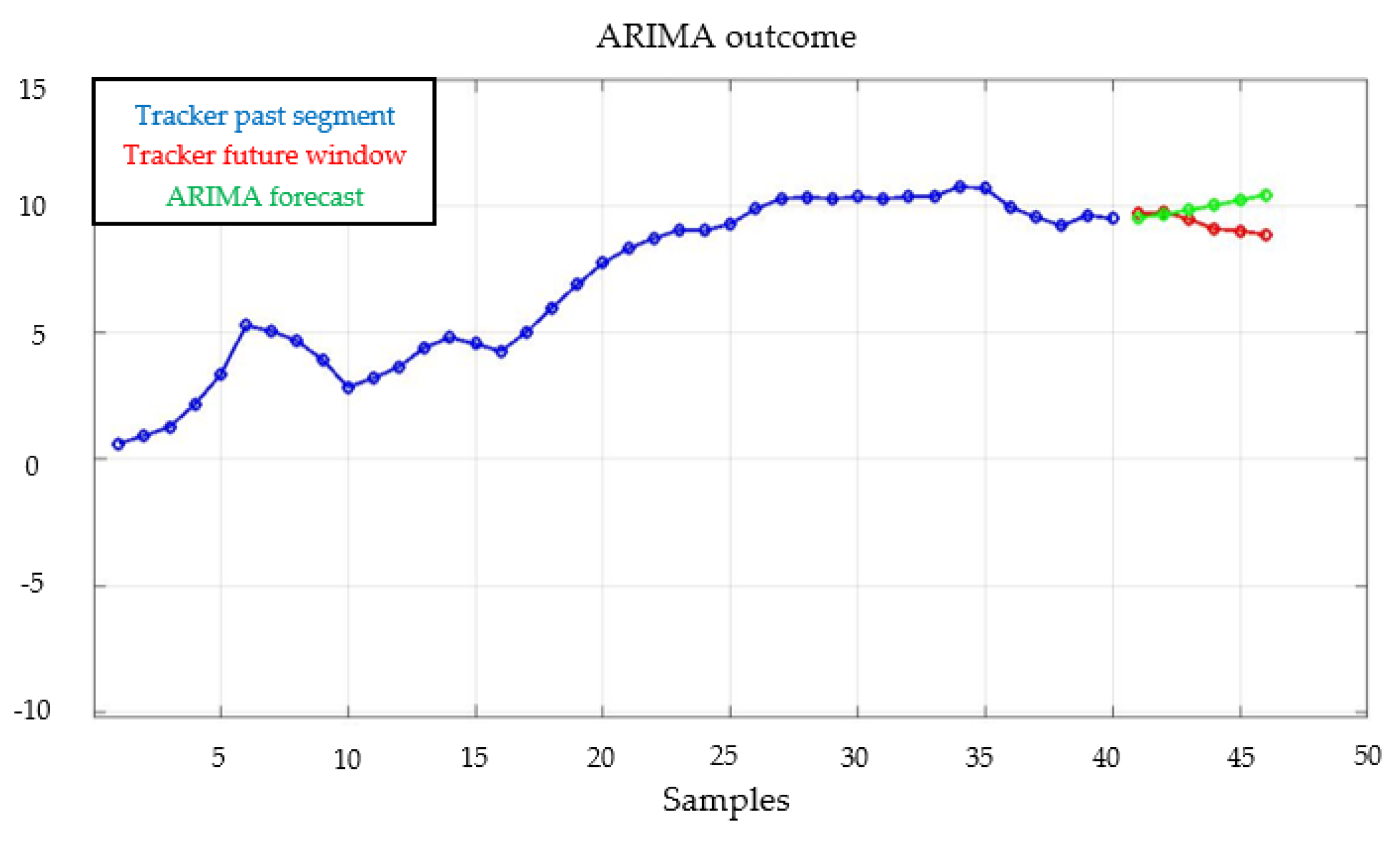
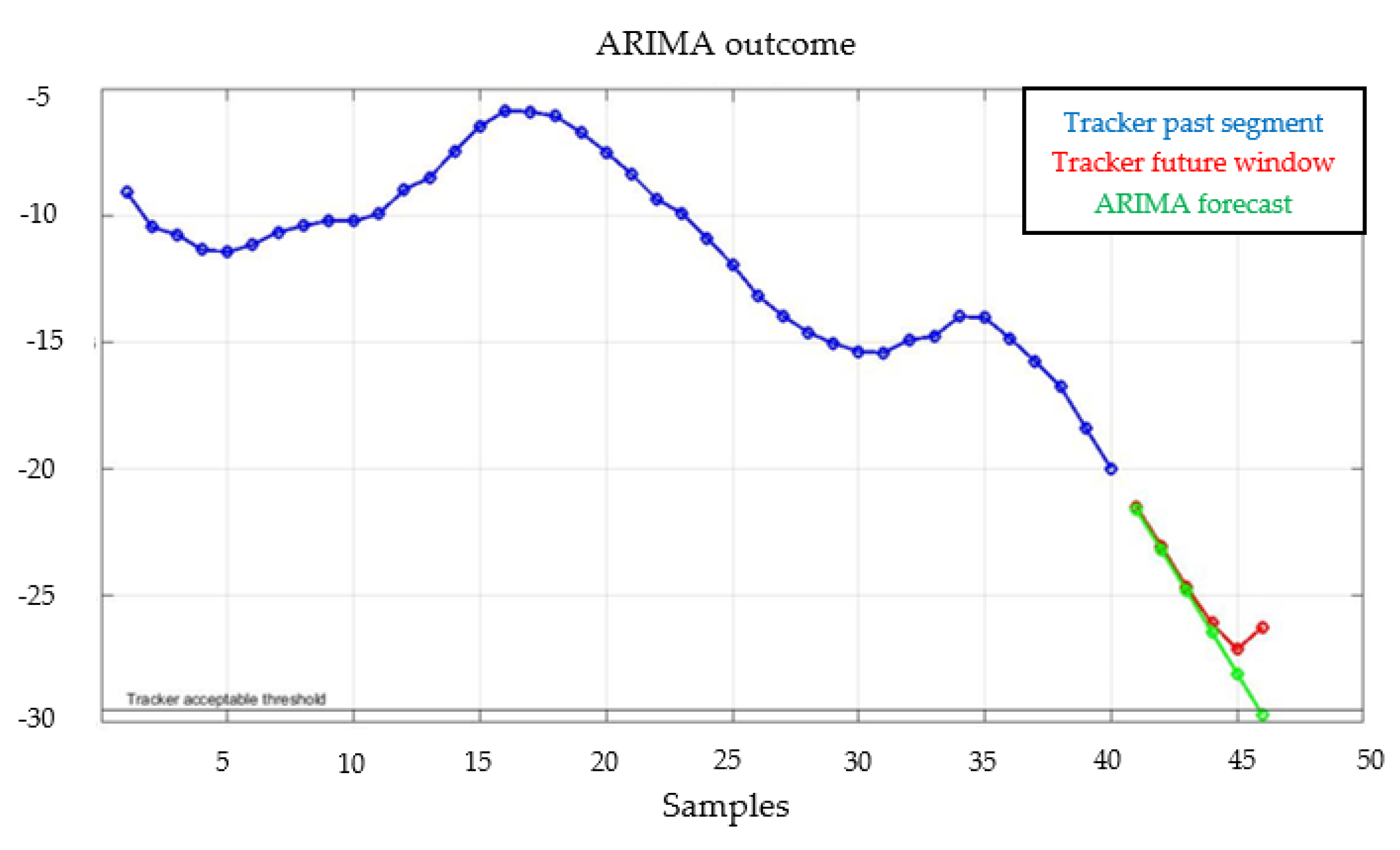
5.2. Application of Customized ARIMA Model

The second stage of the algorithm is the application of the ARIMA model to the tracker time series t to forecast its immediate future tendency. An ARIMA model is actually the sum of three models: AR stands for Autoregressive, I stands for Integrated and MA stands for Moving Average. The Integrated model can be seen just as an auxiliary tool used to satisfy the assumptions of the remaining two ones, and it will be treated later on. The core model is the ARMA one [39]. An ARMA(p,q) model is the sum of an Autoregressive model of order p (Equation (3)) and a Moving Average model of order q (Equation (4)), resulting in the global shape of (Equation (5)). In these equations, X is the modeled variable, meaning the tracker t, Z is a random variable characterized by a normal distribution (Equation (6)) and ϕ and ϑ are the coefficients of the learner.

X_t = ϕ₁ X_t−1 + ⋯ + ϕ_p X_t−p AR(p) model

(3)

X_t = Z_t − ϑ₁Z_t−1 − … − Z_t−q MA(q) model

(4)

X_t = ϕ₁X_t−1 + ⋯ + ϕ_pX_t−p + Z_t − ϑ₁Z_t−1 − … − ϑ_qZ_t−q ARMA(p,q) model

(5)

Z_t ∽ N(0,σ ²)

(6)

In the classical fields of application of ARMA modeling, namely economics and finance, measurements are spaced by time windows of months or years. In this way, the typical length of the entire time series does not overcome 10² points and it is reasonable to model it in a single step, e.g. through Box–Jenkins method [40]. On the other hand, the studied industrial databases reach also 10⁴–10⁵ points and, despite data aggregation, the final length results definitively bigger than the previously mentioned one. Therefore, a single model could never be accurate enough to describe the entire series. Moreover, since the general tendency of the assembly process is to keep a planar behavior, a model built on the entire data history will generate flat and, consequently, meaningless results, precluding the capability of forecasting any problem. To obtain effective and reliable forecasts, this work suggests to model the series step-by-step, considering only the last L points of the whole data sequence, to weight in a stronger way the appearance of anomalies. Of course, for the sake of feasibility, each passage must be automated, to avoid continuous manual tuning of ARIMA orders.

The rest of this sub-section is devoted to explaining the functioning of the algorithm when facing the generic kth portion of the time series. The sequence of operations executed by the algorithm at each iteration is schematized in Figure 5. This procedure is specifically built for the Bosch VHIT S.p.A. assembly systems, therefore presented ARIMA model is customized for such a kind of system.

The very first step is the extraction of the general kth segment of the tracker time series. It can be defined as the data portion going from sample k-L to sample k. Applying the proposed algorithm on it, one should be able to forecast with an acceptable level of accuracy samples going from k + 1 to k + F. Values of L and F must be optimized through SA in order to minimize forecasting error and to maximize model reliability.

Once it is possible to work on the local portion of time series only, ARIMA basic assumptions should be assessed before applying it. The assumptions of the ARIMA model are basically three: the process must not be a white noise, the process must be stationary, the process must be invertible [41]. To solve this aim, statistical inference and, in particular, null hypothesis significance tests (NHST), will be highly exploited.

Firstly, time series non-randomness is assessed through a Ljung-Box Q-Test [40]. In case the kth segment of the tracker results to be a white noise, no useful predictions can be extracted from it and the analyst is forced to move to next segment. Despite this consideration, time series randomness (and consequent ARIMA failure) can be seen as a good point, since it assesses data series flatness and system’s stability.

Secondly, time series stationarity is assessed through the augmented Dickey–Fuller Test [37]. If the test suggests a non-stationary time series, it is differentiated to remove non-stationary trends. The procedure is repeated iteratively until the dth differentiated time series is stationary. Parameter d, namely the number of differentiations, will be the order of the not yet discussed Integrated model of ARIMA. Specifying parameter d, almost all analysis software can differentiate time series, apply ARMA and integrate automatically. In this way, the user can apply ARIMA on the original time series, observing its outcome directly on it and not on the differentiated one. Once assumptions have been assessed and order d has been selected, user’s effort should be focused in selecting orders p, q of the remaining two models. The choice of optimal p, q values is solved through the Bayesian Information Criterion (BIC) application [42], which is an improvement of the classical criterion for model’s parameters optimization, namely the maximum likelihood criterion [40]. The application of ARIMA model with the selected values of p, q does not ensure the proper functioning of the algorithm, because the process could be non-invertible. Typically, this condition holds if q ≥ p and a decrease in the MA model order is sufficient to avoid the problem. Thus, ARIMA is tested with the parameters suggested by BIC and, if it results to be non-invertible, q is lowered until the problem vanishes.

The last step of the kth iteration is the forecast and the evaluation of performances. The idea of coupling some performance indicators to the ARIMA outcome rises because of the separated modeling dedicated to each segment of the time series. This strategy could lead to different modeling performances, depending on the considered segment and each alarm could be more or less reliable. The availability of immediate performance indexes can help the user in quantifying it. In particular, two indicators are used. The first one describes the goodness-of-fit of the model. Basically, it is the output of the Ljung-Box Q-Test applied on the residuals between original time series and model. Randomness of residuals indicates a satisfying goodness-of-fit of the model. The second one describes the forecast reliability and it is represented by the Prediction Mean Square Error (PMSE) [40]. Once forecast has been generated, k is increased of one unit and the algorithm moves to the next iteration (see again Figure 5).

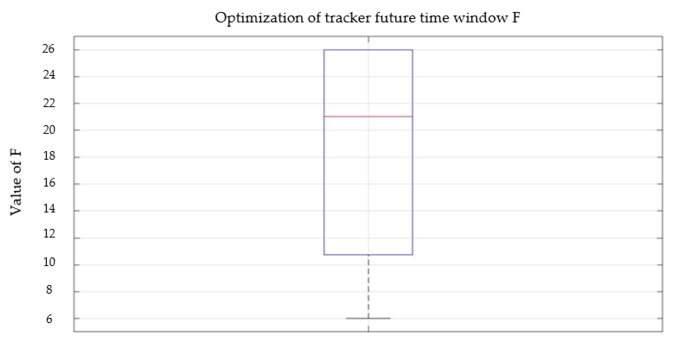
5.3. Parameters Optimization

The last point to be investigated is the optimization of parameters of Table 1 through the application of the SA procedure for assembly systems, which is composed by three consecutive stages, as shown in Figure 6.

The first optimization stage is devoted to ensure the reliability of the tracker, namely its capability to model process’ physics in a reasonable way, by selecting the most appropriate values of N, M, S and, consequently of tracker admissible threshold, T. In particular, it is clever to maximize its capability of being flat in case of nominal operative conditions and of presenting peaks in case of novelty appearance. The proper fulfilment of this first optimization problem is fundamental to ensure a meaningful linkage between the artificial nature of the tracker and the physics of the system. If the tracker cannot be nominally planar and clearly capable of highlighting anomalies, even a precise forecast of it through ARIMA model will be useless.

The second stage is devoted to choose the best value of L to maximize the model’s goodness-of-fit. For each value of L, g time series segments are randomly chosen. BIC maximum value is computed for each segment and the mean value is considered as goodness-of-fit indicator. The idea of repeating g times each iteration rises to perform a capability analysis transcending from the local random sample and able to avoid the consideration of partial or fake results.

The last optimization stage is used to choose the best value of F. Of course, the higher is F, the higher is the achievable advance but, on the other hand, the higher is the forecasting error. Therefore, the idea is to try with ascending values of F until a non-acceptable threshold for the error is passed. A standard acceptable threshold for the PMSE is 10%. As in optimization stage 2, g random tests are repeated for each selection of F, in order to achieve more reliable results.

Section 6 shows the results after the application of the customized KDD-ARIMA methodology.

6. Results

This section reports the results obtained through the application of the customized KDD-ARIMA methodology to the Bosch VHIT S.p.A. assembly system. The goal is to control the production and to anticipate, if possible, any unforeseeable issue. In particular, in Section 6.1, results are shown in the details for one successful case, for which the developed algorithm, after a ramp-up phase to set up the model parameters, finally is able to forecast a deviation in the production process up to 13 hours before the issue appears. This result comes from the application of the customized KDD-ARIMA tool on historical data. However, its effectiveness is demonstrated also with other applications, summarized in Section 6.2, and now the industrialization of the model is ongoing inside the enterprise. The idea is to let it work continuously on a dedicated server for controlling purposes of the production process within the assembly department of Bosch VHIT S.p.A.

6.1. Customized KDD Application

This problem has affected the workstation devoted to a diesel gear pump functional test. The seal of a valve connected to the pneumatic system of the station starts wearing, resulting in air losses and in a decrease of the air flow rate observed during processing of pumps, as shown in Figure 7. Thus, this is an example of how a technical issue is indirectly observed from process parameters’ viewpoint.

KDD-ARIMA based framework has been applied to the considered variable. The outcome of SA 1-st stage is the optimal tracker series, having the shape described in Figure 8, while the remaining two stages provide the outputs described in Figure 9 and Figure 10. For each value of L and F, it was decided to adopt g = 25 since this is the typical number of tests used in the plant for capability and R&R checks.

Results obtained applying ARIMA modeling with previously tuned parameters on the considered case study, are really interesting. Firstly, no fake alarms have been signaled by the tool. Secondly, all segments resulting in being white noises belong to a situation of nominal productive conditions. Therefore, the functioning of the algorithm is not compromised. Thirdly, the decreasing flow rate has been captured with a great advance. In particular, knowing the real moment in which the current alarm system has been activated, it is possible to quantify this advance. Specifically, the alarm has been anticipated of 880 pieces, corresponding to almost 13 h of production. This means that the warning provided by proposed tool would have been able to allocate maintenance resources to troublesome workstation 13 h before the actual realization of the problem, allowing a preventive intervention and avoiding the concretization of the problem. From an economic point of view, considering the damages due to both fake scraps generated during the rising of the issue and the production stop to implement corrective action, the usage of proposed tool, according to estimates made by the company, could have saved at least 60,000 € per predicted issue.

Figure 11 and Figure 12 show the predictive performances of the algorithm in the cases of nominal operative conditions and rising anomaly. Looking at these two graphs, it is possible to notice that the prediction appears much more accurate in correspondence of the novelty. This is clearly due to the rising of a deterministic phenomenon. Therefore, according to this statement and to the fact that random noise segments appear in the case of nominal production only, it is possible to conclude that the algorithm works better in case of appearance of a novelty. This point can be considered as an additional assessment of algorithm’s reliability.

6.2. Summary of Other Customized KDD Applications

The customized KDD-ARIMA methodology have been applied to different lines of the Bosch VHIT S.p.A. assembly system. A small recap is provided in

Table 3. Advance achievable with proposed tool with respect to original warning systems on both technical and qualitative issues.

Problem	Nature of the Issue	Affected Process Parameter	Algorithm’s Performance	N	M	L	F
Obstruction of a pipe due to engine oil drops	Technical	Air volumetric flow rate	Identification in advance of 61 h	800	100	20	8
Porosity in pump’s channels	Qualitative	Air volumetric flow rate	Identification in advance of 2.3 h	100	10	40	4
Wear and sliding of a spindle	Technical	Torque absorbed by the pump	Identification in advance of 16 h	400	40	40	6
Non-compliant material of screws	Qualitative	Screwing torque	Identification in advance of 1.3 h	750	100	30	5

to prove the repeatable goodness of tested methodology.

7. Conclusions

Three main results are achieved, according to the gaps found in academic literature and the experience gathered from the industrial environment within Bosch VHIT S.p.A.

Firstly, a well-defined and standardized Industrial Big Data Analytics procedure for the control of assembly systems is developed:

• Exploitation of data analysis in assembly environment. Literature research has revealed a high imbalance between research effort in studying machining data and assembly ones, in favor of the first category. This work could help in reducing this gap.
• Standardized and flexible framework of the presented procedure. The KDD-based backbone of the process, together with the systematic rules provided in each section of the process, gives it a standardized nature, fundamental to allow its full-scale implementation in the manufacturing world. On the other hand, the iterative and parametric policies adopted on different layers of the procedure leave some degrees of freedom with respect to its general architecture, allowing to customize it.
• Definition of rigorous and effective guidelines in data mining algorithms’ selection. The two-stage selection technique proposed in Section 4.5 appears as a powerful guideline devoted to the minimization of user’s effort in the choice and application of statistical learning algorithms.

Secondly, the ARIMA-based predictive model is applied and validated. The application of the proposed tool on several cases related to a real and consolidated manufacturing environment demonstrates that it is actually able to provide tangible gains, by identifying rising issues with consistent advances and by demolishing consequent failure costs.

Third, the application of the KDD-ARIMA methodology has shown important results in terms of time and economic savings from a practical perspective, underlining how the developed methodology may able to increase the economic performance of the company. To conclude, Bosch VHIT S.p.A. is pushing towards the application of such methodology on all of its assembly lines, stressing the impact this work has and confirming the interest of practitioners.

Future Work

The proposed work is eligible for further exploitation, both to improve the potentiality of the proposed KDD methodology and to industrialize the solution to cover all the assembly lines of the company. Thus, future effort should be focused on:

• Research for alternative algorithms satisfying the two-stage selection procedure discussed in Section 4.5. The target should be the comparison and the assessment of the proposed algorithm (ARIMA) with respect to alternative ones or its eventual replacement with more satisfactory solutions. This point is mainly driven by the extremely wide range of methods contained within novelty detection literature that must be investigated when applied to manufacturing environments.
• Research for tools able to work on entire assembly systems instead of single process parameters. Even though this work is focused on single variables, according to needs of the company and to physics of their processes, in other scenarios, relationships between different parameters may exist, pushing towards the identification of hidden patterns. A possible target for this kind of system could be the creation of a “Digital Check”, namely an instrument able to predict the outcome of a certain workstation by analyzing the outcomes of previous ones.
• Research for architectures able to industrialize the presented methodology in a structured way. Tools such as a Decision Support System (DSS), with high degrees of automation and easy implementation on company’s Manufacturing Execution System (MES), could be a reasonable solution for companies deciding to adopt implement the presented solution [43,44,45,46,47].

References

1. Shin, J.H.; Jun, H.B. On condition based maintenance policy. J. Comput. Des. Eng. 2015, 2, 119–127. [Google Scholar] [CrossRef]
2. Goel, P.; Datta, A.; Sam Mannan, M. Industrial alarm systems: Challenges and opportunities. J. Loss Prev. Process Ind. 2017, 50, 23–26. [Google Scholar] [CrossRef]
3. Jiang, Y.; Yin, S. Recursive total principle component regression based fault detection and its application to Vehicular Cyber-Physical Systems. IEEE Trans. Ind. Inf. 2018, 4, 1415–1423. [Google Scholar] [CrossRef]
4. Jiang, Y.; Yin, S.; Kaynak, O. Data-driven Monitoring and Safety Control of Industrial Cyber-Physical Systems: Basics and Beyond. IEEE Access 2018, 6, 47374–47384. [Google Scholar] [CrossRef]
5. Bumbaluskas, D.; Gemmill, D.; Igou, A.; Anzengruber, J. Smart Maintenance Decision Support System (SMDSS) based on corporate data analytics. Expert Syst. Appl. 2017, 90, 303–317. [Google Scholar] [CrossRef]
6. Ge, Z.; Song, Z.; Ding, D.X.; Haung, A.B. Data Mining and analytics in the process industry: The role of machine learning. IEEE Access 2017, 5, 20590–20616. [Google Scholar] [CrossRef]
7. Mourtzis, D.; Vlachou, K.; Milas, N. Industrial Big Data as a result of IoT adoption in manufacturing. Procedia CIRP 2016, 55, 290–295. [Google Scholar] [CrossRef]
8. Kranz, M. Building the Internet of Things: Implement New Business Models, Disrupt Competitors, Transform Your Industry; John Wiley & Sons Inc.: Hoboken, NJ, USA, 2016. [Google Scholar]
9. Tiwari, S.; Wee, H.M.; Daryanto, Y. Big data analytics in supply chain management between 2010 and 2016: Insights to industries. Comput. Ind. Eng. 2018, 115, 319–330. [Google Scholar] [CrossRef]
10. Piateski, G.; Frawley, W. Knowledge Discovery in Databases; MIT Press: Cambridge, MA, USA, 1991. [Google Scholar]
11. Gamarra, C.; Guerrero, J.M.; Montero, E. A knowledge discovery in databases approach for industrial microgrid planning. Renew. Sustain. Energy Rev. 2016, 60, 615–630. [Google Scholar] [CrossRef] [Green Version]
12. Cheng, G.Q.; Zhou, B.H.; Li, L. Integrated production, quality control and condition-based maintenance for imperfect production systems. Reliab. Eng. Syst. Saf. 2018, 175, 251–264. [Google Scholar] [CrossRef]
13. Mourtzis, D.; Vlachou, E. A cloud-based cyber-physical system for adaptive shop-floor scheduling and condition-based maintenance. J. Manuf. Syst. 2018, 47, 179–198. [Google Scholar] [CrossRef]
14. Kumar, S.; Goyal, D.; Dang, R.K.; Dhami, S.S.; Pabla, B.S. Condition based maintenance of bearings and gearsfor fault detection—A review. Mater. Today 2018, 5, 6128–6137. [Google Scholar] [CrossRef]
15. Bengtsson, M.; Kurdve, M. Machining Equipment Life Cycle Costing Model with Dynamic Maintenance Cost. Procedia CIRP 2016, 48, 102–107. [Google Scholar] [CrossRef]
16. Keliris, C.; Polycarpou, M.; Parisini, T. A distributed fault detection filtering approach for a class of interconnected continuous-time nonlinear systems. IEEE Trans. Autom. Control 2013, 58, 2032–2047. [Google Scholar] [CrossRef]
17. Mahmoud, M.; Shi, P. Robust Kalman filtering for continuous time-lag systems with markovian jump parameters. IEEE Trans. Circuits Syst. 2003, 50, 98–105. [Google Scholar] [CrossRef]
18. Nahmias, S.; Lennon Olsen, T. Production and Operations Analysis; Waveland Press Inc.: Long Grove, IL, USA, 2015. [Google Scholar]
19. Fayyad, U.; Stolorz, P. Data mining and KDD: Promise and challenge. Future Gener. Comput. Syst. 1997, 13, 99–115. [Google Scholar] [CrossRef]
20. Gullo, F. From Patterns in Data to Knowledge Discovery: What Data Mining can do. Phys. Procedia 2015, 62, 18–22. [Google Scholar] [CrossRef]
21. Galar, D.; Kans, M.; Schmidt, B. Big Data in Asset Management: Knowledge Discovery in Asset Data by the Means of Data Mining. In Proceedings of the 10th World Congress on Engineering Asset Management, Tampere, Finland, 28–30 September 2015. [Google Scholar]
22. Choudhary, A.K.; Harding, J.A.; Tiwari, M.K. Data Mining in manufacturing: a review based on the kind of knowledge. Adv. Eng. Inf. 2008, 33, 501. [Google Scholar] [CrossRef] [Green Version]
23. Qu, Z.; Liu, J. A new method of power grid huge data pre-processing. Procedia Eng. 2011, 15, 3234–3239. [Google Scholar] [CrossRef]
24. Bilalli, B.; Abellò, A.; Aluja–Banet, T.; Wrembel, R. Intelligent assistance for data pre-processing. Comput. Stand. Interfaces 2017, 57, 101–109. [Google Scholar] [CrossRef]
25. Munson, M.A. A study on the importance of and time spent on different modeling steps. ACM SIGKDD Explor. Newsl. 2011, 13, 65–71. [Google Scholar] [CrossRef]
26. Garces, H.; Sbarbaro, D. Outliers detection in industrial databases: An example sulphur recovery process. World Congr. 2011, 18, 1652–1657. [Google Scholar] [CrossRef]
27. Nisbet, R.; Miner, G.; Yale, K. Handbook of Statistical Analysis and Data Mining Applications; Academic Press: Burlington, MA, USA, 2018. [Google Scholar]
28. Gandomi, A.; Haider, M. Beyond the hype: Big Data concepts, methods and analytics. Int. J. Inf. Manag. 2014, 35, 137–144. [Google Scholar] [CrossRef]
29. Saporta, G.; Niang, N. Data Analysis; ISTE Ltd.: London, UK, 2009; pp. 1–23. [Google Scholar]
30. James, G.; Witten, D.; Hastie, T.; Tibshirani, R. An Introduction to Statistical Learning; Springer: New York, NY, USA, 2013. [Google Scholar]
31. Hastie, T.; Tibshirani, R.; Friedman, J. The elements of Statistical Learning; Springer: New York, NY, USA, 2001. [Google Scholar]
32. Pimentel, M.A.F.; Clifton, D.A.; Clifton, L.; Tarassenko, L. A review of novelty detection. Signal Process. 2014, 99, 215–249. [Google Scholar] [CrossRef]
33. Amhmad, S.; Lavin, A.; Purdy, S.; Agha, Z. Unsupervised real-time anomaly detection for streaming data. Neurocomputer 2017, 262, 134–147. [Google Scholar] [CrossRef] [Green Version]
34. Baptista, M.; Sankararaman, S.; de Medeiros, I.P.; Nascimento, C.Jr; Prendiger, H.; Henriques, E.M.P. Forecasting fault events for predictive maintenance using data-driven techniques and ARMA modeling. Comput. Ind. Eng. 2018, 115, 41–53. [Google Scholar] [CrossRef]
35. Janouchová, E.; Kučerová, A. Competitive comparison of optimal designs of experiments for sampling-based sensitivity analysis. Comput. Struct. 2013, 124, 47–60. [Google Scholar] [CrossRef] [Green Version]
36. Barreiro, P.L.; Albandoz, J.P. Population and sample. Sampling techniques. Available online: https://www.google.com/url?sa=t&rct=j&q=&esrc=s&source=web&cd=1&ved=2ahUKEwi9kez10ebdAhWOyKQKHXmvCVMQFjAAegQIBxAC&url=https%3A%2F%2Foptimierung.mathematik.uni-kl.de%2Fmamaeusch%2Fveroeffentlichungen%2Fver_texte%2Fsampling_en.pdf&usg=AOvVaw2btopZugJaU8jsfUXEfm2l (accessed on 2 October 2018).
37. French, A.; Chess, S. Canonical Correlation Analysis & Principal Component Analysis. Available online: http://userwww.sfsu.edu/efc/classes/biol710/pca/CCandPCA2.htm (accessed on 2 October 2018).
38. Chen, K.; Wang, J. Design of multivariate alarm systems based on online calculation of variational directions. Chem. Eng. Res. Des. 2017, 122, 11–21. [Google Scholar] [CrossRef]
39. Neusser, K. Time Series Econometrics; Springer: New York, NY, USA, 1994. [Google Scholar]
40. Model Selection. In Econometrics ToolboxTM User’s Guide; The MathWorks Inc.: Natick, MA, USA, 2001.
41. Statistics ToolboxTM User’s Guide; The MathWorks Inc.: Natick, MA, USA, 2016.
42. Woods, D.C.; McGree, J.M.; Lewis, S.M. Model selection via Bayesian information capacity designs for generalized linear models. Comput. Stat. Data Anal. 2016, 113, 226–238. [Google Scholar] [CrossRef]
43. Prasad, D.; Ratna, S. Decision support systems in the metal casting industry: An academic review of research articles. Mater. Today Proc. 2018, 5, 1298–1312. [Google Scholar] [CrossRef]
44. Krzywicki, D.; Faber, L.; Byrski, A.; Kisiel-Dorohinicki, M. Computing agents for decision support systems. Future Gener. Comput. Syst. 2014, 37, 390–400. [Google Scholar] [CrossRef] [Green Version]
45. Li, H.; Pang, X.; Zheng, B.; Chai, T. The architecture of manufacturing execution system in iron & steel enterprise. IFAC Proc. Vol. 2005, 38, 181–186. [Google Scholar]
46. Jiang, P.; Zhang, C.; Leng, J.; Zhang, J. Implementing a WebAPP-based Software Framework for Manufacturing Execution Systems. IPAC-Pap. Online 2015, 48, 388–393. [Google Scholar] [CrossRef]
47. Itskovich, E.L. Fundamentals of Design and Operation of Manufacturing Executive Systems (MES) in Large Plants. IPAC Proc. Vol. 2013, 46, 313–318. [Google Scholar] [CrossRef]
Figure 1. Exploitation of IIoT potential through Big Data Analytics in the main market sectors.
Machines 06 00045 g001
Figure 2. Logical structure of a general KDD process for which raw data are the global input.
Machines 06 00045 g002
Figure 3. Bosch VHIT S.p.A. actual flow of data.
Machines 06 00045 g003
Figure 4. Time series of the air volumetric flow rate measured within a vacuum pump to test presence of leakages. The typical behavior is flat while the peculiar behavior rising at the end of the sequence corresponds to an issue observed in the pneumatic circuit of the bench.
Machines 06 00045 g004
Figure 5. Proposed algorithm’s functioning for general kth iteration. Models’ orders p, d, q are automatically set through statistical inference hypothesis tests, in order to avoid manual intervention.
Machines 06 00045 g005
Figure 6. Procedure adopted to optimize parameters feeding the discussed algorithm.
Machines 06 00045 g006
Figure 7. Time series of measured air flow rate. The degradation of an o-ring, a round gasket aimed at preserve air leakages, generates a decreasing path until the lower acceptable bound trespasses and the station starts discharging products. Each point represents a processed product.
Machines 06 00045 g007
Figure 8. Optimal tracker time series (green curve) vs. number of scraps per sample (red curve), referring to flow rate of Figure 10. The outcome of SA first step suggests to use N = 400, M = 40, T = −29.5237 and to combine μ, σ, Pu, Pl, Cpu, Cpl, θ, Δ to build the tracker. Each point represents the tracker value for a sample of N products while the black line stands for the admissible threshold computed for the tracker.
Machines 06 00045 g008
Figure 9. Optimization stage for tracker segment length L. Values from 20 to 100, with a shift of 10 between two attempts, have been tested. L = 40 is selected since it maximizes BIC. Each value is repeated g = 25 times and the statistical distribution of corresponding results is provided in the associated box plot.
Machines 06 00045 g009
Figure 10. Optimization stage for future window F. g = 25 values of F ensuring PMSE < 10% have been tested. F = 6 (minimum) has been selected to be conservative and to avoid fake alarms.
Machines 06 00045 g010
Figure 11. Algorithm’s forecast (green line) against real tracker behavior (red line), in the case of nominal operative conditions (sample 83 of tracker time series).
Machines 06 00045 g011
Figure 12. Algorithm’s forecast (green line) against real tracker behavior (red line), when the valve starts wearing (sample 210 of tracker time series). The passing of tracker acceptable threshold determines the warning given by the code.
Machines 06 00045 g012