Joint Optimization of Preventive Maintenance, Spare Parts Inventory and Transportation Options for Systems of Geographically Distributed Assets

Abstract

Maintenance scheduling for geographically dispersed assets intricately and closely depends on the availability of maintenance resources. The need to have the right spare parts at the right place and at the right time inevitably calls for joint optimization of maintenance schedules and logistics of maintenance resources. The joint decision-making problem becomes particularly challenging if one considers multiple options for preventive maintenance operations and multiple delivery methods for the necessary spare parts. In this paper, we propose an integrated decision-making policy that jointly considers scheduling of preventive maintenance for geographically dispersed multi-part assets, managing inventories for spare parts being stocked in maintenance facilities, and choosing the proper delivery options for the spare part inventory flows. A discrete-event, simulation-based meta-heuristic was used to optimize the expected operating costs, which reward the availability of assets and penalizes the consumption of maintenance/logistic resources. The benefits of joint decision-making and the incorporation of multiple options for maintenance and logistic operations into the decision-making framework are illustrated through a series of simulations. Additionally, sensitivity studies were conducted through a design-of-experiment (DOE)-based analysis of simulation results. In summary, considerations of concurrent optimization of maintenance schedules and spare part logistic operations in an environment in which multiple maintenance and transpiration options are available are a major contribution of this paper. This large optimization problem was solved through a novel simulation-based meta-heuristic optimization, and the benefits of such a joint optimization are studied via a unique and novel DOE-based sensitivity analysis.

1. Introduction

For geographically distributed systems of degrading assets and maintenance facilities serving these assets, such as assets and maintenance facilities in airlines and oil/gas extraction companies, preventive maintenance (PM) scheduling is a challenging decision-making problem because of its inherent interactions with the availability of the required maintenance resources. As PM operations are aimed at ensuring the assets’ availability by replacing degraded parts before they actually fail, getting the right amounts and types of spares parts to the right places at the right time is of paramount importance for a successful PM execution. Therefore, the spare parts logistics (SPL), including inventory levels in maintenance facilities and the transportation options to deliver the spare parts, should be considered along with the maintenance schedules.

According to a recent review [1], the existing works on joint scheduling of PM and SPL mainly focus on the optimization of reliability-based maintenance policies in a spare parts inventory system. From the side of maintenance, both the age-based (usage-based) [2,3,4,5] and block-based (period-based) PM policies [6,7,8,9] are considered. In addition, several recent studies considered joint PM and SPL decision-making for advanced asset systems, such as a serial-connected multi-part asset structure [10,11,12], k-out-of-n asset structure [13,14], flexible-connect multi-part asset structure [15], and simple asset structure with multiple failure modes [16].

From the side of SPL, joint decision-making problems have been considered in both continuous-review inventory systems [2,3,15] and periodical-review inventory systems [9,12]. These works evaluated several inventory management strategies, including the periodic review inventory replenishment policy (often referred to in the SPL literature as the “(R, S) replenishment policy”) [9,17], the so-called min–max replenishment policy (often referred to in the SPL literature as the “(s, S) replenishment policy”) [2,3,5,16], and the strategy with reserved inventories for PMs [18]. Beyond inventory management, the authors of [19,20] extended the definition of the maintenance resource by considering technicians of different skill levels, thus involving the human resource planning into the resulting decision-making policies, while Chen et al. [21] assumed the existence of multiple suppliers and proposed an integrated decision-making policy for the resulting multi-echelon logistic network.

Sensitivity studies for the integrated PM and SPL decision-making policies have also received attention in the literature [4,12,17]. These sensitivity studies are inspired by parametric uncertainties that often cannot be directly evaluated and have to be estimated based on the expert knowledge or extended observation of the system [22,23]. Generally speaking, there is still the lack of a well-established methodological approach to quantitatively study the effects of changing system parameters and to fully understand their interactions in the decision-making process. To that end, a design-of-experiment (DOE)-based approach to study the effects and interactions between various system parameters on the decision-making process and its performance seems to be a highly plausible and elegant solution option [24].

In this paper, we introduce an integrated decision-making process that jointly optimizes PM schedules, spare part inventory levels, and transportation options for spare parts in a geographical dispersed network of multi-part assets and multi-level maintenance facilities serving those assets with the necessary spare parts. More specifically, we consider concurrent optimization of maintenance schedules and SPL operations in an environment consisting of multiple geographically dispersed assets, each of which consists of multiple components that degrade according to asset- and component-specific reliability functions (which is needed because the same component in a different asset may degrade differently because of a different usage pattern), with stochastic route-dependent spare part delivery times and multiple maintenance and transpiration options being available. This detailed and realistic integrated model of maintenance and SPL operations will be implemented and solved via discrete-event simulations and represents a unique contribution of this paper. In addition, benefits of the novel integrated approach will be studied through a DOE-based sensitivity analysis, which enables the statistical determination of the effects of various system parameters and their interactions on the decision-making process and its performance. A similar idea is presented by the authors of [24], who use space-filling DOE and the concept of expected value of perfect information (EVPI) as a measure of sensitivity to study the sensitivity of optimized preventive maintenance decisions with respect to changes in model parameters. However, the concept of a DOE-based sensitivity analysis has not yet been utilized in joint maintenance and SPL decision-making, and will be employed in that domain for the first time in this paper.

The rest of the paper is organized as follows. Section 2 describes joint PM and SPL decision-making in the form of a stochastic optimization formulation. Section 3 introduces a simulation-based meta-heuristic approach to solving the optimization problem described in Section 2. In Section 4, the proposed integrated decision-making process is evaluated in a simulated environment, using a DOE-based sensitivity analysis. Section 5 provides conclusion of this research and outlines several possible avenues for future work.

2. Methodology

2.1. Problem Statement

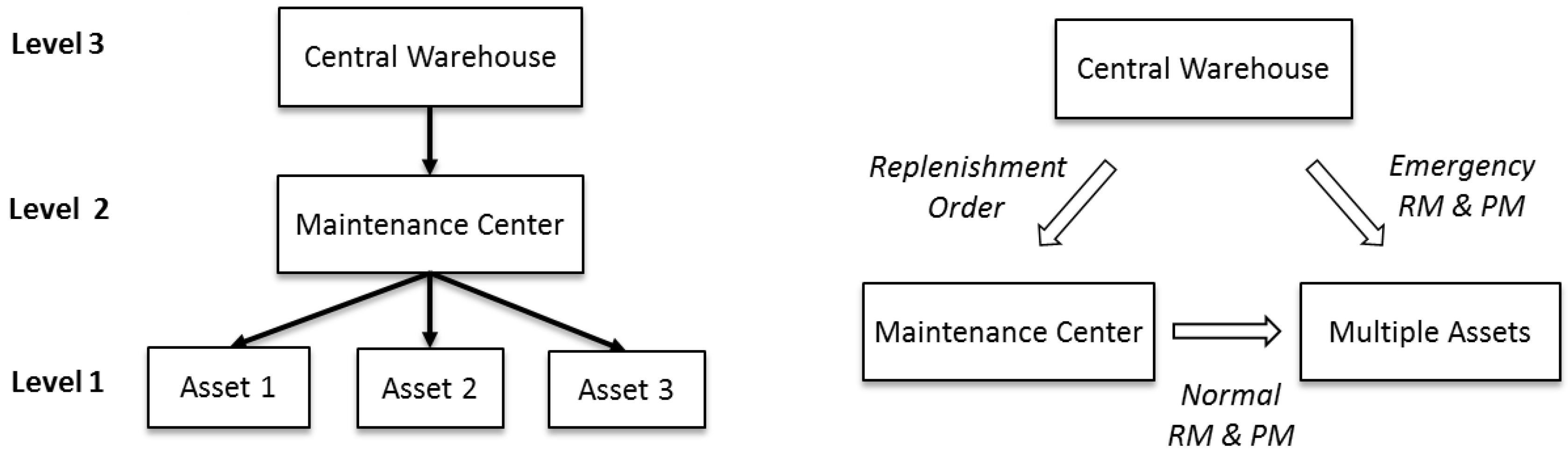
As illustrated in Figure 1, the topology of the SPL system considered in this paper is a three-level logistic network, consisting of a central warehouse, a maintenance center, and a set of multiple assets. Furthermore, the assets are assumed to have multi-part structure, each consisting of multiple independent working parts. These entities are explained in more detail below.

• A central warehouse is the primary source for all new spare parts and plays two roles in the spare part inventory flow—replenishing spare parts for the maintenance centers following a (s, S) replenishment policy [25], or providing spare parts directly to the assets as emergency orders when the maintenance order could not be satisfied from a maintenance center. Infinite inventory levels of spare parts are assumed for the central warehouse.
• A maintenance center fulfills maintenance orders from the nearby assets by shipping new undegraded spare parts to their operating sites. It is assumed to have finite inventory levels of spare parts and any maintenance order that cannot be immediately fulfilled by the maintenance center is serviced via an emergency order to the central warehouse.
• The term asset is used to refer to a machine that can be operated independently to generate revenue. It is assumed that there is a fleet of geographically dispersed assets in the system, labeled $A_1,A_2,\dots ,A_J$. An asset consists of multiple independent working parts and can only operate properly if all its parts behave properly.
• The term working part is used to refer to a basic unit of an asset. An asset $A_j$ ($1\le j\le J$) is assumed to be made up of $K_j$ serially connected parts, labeled $P_{j,1},P_{j,2},\dots ,P_{j,K_j}$. Degradation process of a part $P_{j,k}$ is characterized by a reliability function, ${\mathcal{D}}_{j,k}(·)$, representing the distribution of that part’s usage time to failure. From the point of view of logistics, a working part on an asset corresponds to a certain type of a spare part that needs to be stored in the maintenance center. During a preventive or reactive maintenance intervention, a new spare part should be shipped either from the maintenance center or directly from the central warehouse to replace the degraded working part.

In this paper, a continuous-review inventory system is considered and an (s, S) replenishment policy is followed to manage spare part inventories in the maintenance centers. Let $S{P}_1, S{P}_2,\dots , S{P}_I$ denote all spare parts needed to be stocked in a maintenance center. For a spare part $S{P}_i$, the re-order inventory level $y_i$ (corresponding to s in the replenishment policy) indicates the critical level of this spare part that triggers a replenishment order with batch size $z_i$ (corresponding to s-S in the replenishment policy), indicating the number of the spare parts to be shipped from the central warehouse to that maintenance center. Furthermore, the replenishment cost per order ($S_i$) is assumed to be a linear function of the batch size ($z_i$), or more formally,

$$S_i\left(z_i\right)=S_i^{fix}+S_i^{add}\ast \left(z_i-1\right)$$

where $S_i^{fix}$ denotes the fixed replenishment handling cost and $S_i^{add}$ denotes the additional cost to have one more spare part added to the replenishment order.

From the side of maintenance decisions, the so-called reactive maintenance policy is assumed [1], that is to say, both PM and reactive (unscheduled) maintenance (RM) intervention involve a new spare part replacing the broken or severely degraded working part on the asset. Moreover, a usage-based PM triggering policy is considered, which means that a PM triggering usage level $x_{j,k}$ is set for each working part $P_{j,k}$, indicating the part’s critical usage level at which a PM operation is initiated.

Once initialized, a complete maintenance order consists of two phases: transportation and execution.

(1) Transportation consists of shipping the ordered spare part to the asset $A_j$ from the maintenance center as a normal order, or from the central warehouse as an emergency order, with the lead times following the distributions $\mathcal{M}{\mathcal{T}}_j(·)$ and $\mathcal{C}{\mathcal{T}}_j(·)$, respectively.

During RMs, a significant portion of the asset downtimes are caused by the waiting times for the new spare part. Therefore, several expedited shipping options will be considered, with faster ones incurring more costs. More formally, decision variable $u_j$ will be used to denote the relative acceleration of the expedited shipping option compared with normal delivery to the asset $A_j$, with its influence on the lead time distributions (though we do not explicitly model holding costs accrued for parts in transport, these costs are present in the model via the transport costs associated with each transport option) and expedited shipping costs as follows:

• Lead time from the maintenance center to $A_j$ following the distribution $\mathcal{M}{\mathcal{T}}_j\left(\left(1+u_j\right)\ast t\right)$.
• Lead time from the central warehouse to $A_j$ following the distribution $\mathcal{C}{\mathcal{T}}_j\left(\left(1+u_j\right)\ast t\right)$.
• Expedited shipping cost to accelerate an RM delivery to the asset $A_j$ given by $T_j\ast u_j$.

Obviously, decision variable $u_j$ scales the delivery times, with, for example, $u_j=0$ corresponding to no acceleration in deliveries, $u_j=1$ doubling the speed of deliveries, $u_j=2$ tripling that speed, and so on.

(2) Execution is essentially the process in which the target part on the asset is replaced with the newly delivered spare part, resulting in a maintenance intervention. The times needed to execute maintenance interventions will be referred to as repair times.

It is assumed that an RM always restores the part $P_{j,k}$ to as-good-as-new condition, or, in other words, RM operations are assumed to be so-called perfect maintenance operations. However, it is assumed that PM operations of various performance qualities are available, with different costs and repair times. The character of a PM on an asset $A_j$ will be described by the PM recovery rate $v_j$, representing its relative quality compared with a perfect PM. The decision variable $v_j$ is assumed to take discrete values between 0 and 1 ($v_j=1$ indicates a perfect PM and $v_j=0$ indicates a minimal repair), influencing the PM-related parameters as follows:

• Usage to failure of the part $P_{j,k}$ after PM following the distribution ${\mathcal{D}}_{j,k}\left(\frac{t}{\left(1-\alpha \right)v_j+\alpha }\right)$.
• PM cost per order on the part $P_{j,k}$ given by $M_{j,k}\left(v_j\right)=M_{j,k}^{fix}+M_{j,k}^{add}\ast v_j$.
• PM repair time on the part $P_{j,k}$ given by $R{T}_{j,k}\left(v_j\right)=R{T}_{j,k}^{fix}+R{T}_{j,k}^{add}\ast v_j$.

In the above, $\alpha >0$ denotes the relative quality of a minimal repair compared to a perfect operation, $M_{j,k}^{fix}$($R{T}_{j,k}^{fix}$) denotes the fixed PM cost (time), and $M_{j,k}^{add}$($R{T}_{j,k}^{add}$) denotes the additional cost (time) to improve PM performance.

2.2. Stochastic Optimization Formulation

In this paper, we will seek an integrated decision-making policy for the usage levels triggering PMs for working parts (please note that we here evaluate just a purely usage-based PM policy, without considerations of other options, such as, e.g., opportunistic maintenance. Such additional maintenance options can be incorporated into the same simulation-based framework, though such considerations remain outside the scope of this paper.) ($x_{j,k}$ − s), re-order and target inventory levels for spare parts being stocked in the maintenance centers ($y_i$ − s and $z_i$ − s), the expedited delivery rates for RMs ($u_j$ − s), and the recovery rates of PMs ($v_j$ − s). More formally, the integrated decision-making policy will be pursued through the following stochastic optimization,

$$\underset{\begin{array}{c}{\left\{x_{j,k}\in X_{j,k}\right\}}_{1\le j\le J, 1\le k\le K_j }\\ {\left\{y_i\in Y_i\right\}}_{ 1\le i\le I}\\ {\left\{z_i\in Z_i\right\}}_{ 1\le i\le I}\\ {\left\{u_j\in U_j\right\}}_{1\le j\le J}\\ {\left\{v_j\in V_j\right\}}_{1\le j\le J}\end{array}}{\mathrm{Minimize}}\frac{1}{T}\mathbb{E}\left\{{\displaystyle \sum }_{1\le i\le I}\left(h_i{H}_i+s_i{S}_i\left(z_i\right)\right)+{\displaystyle \sum }_{\begin{array}{c}1\le j\le J\\ 1\le k\le K_j\end{array}}\left(r_{j,k}{R}_{j,k}+m_{j,k}{M}_{j,k}\left(v_j\right)+e_{j,k}{E}_{j,k}\right)+{\displaystyle \sum }_{1\le j\le J}{l}_j{L}_j+{\displaystyle \sum }_{\begin{array}{c}1\le j\le J\\ 1\le k\le K_j\end{array}}{r}_{j,k}{T}_j·u_j\right\}$$

(1)

where the terms are explained in

Table 1. Notation used in the optimization Formulation (1). PM—Preventive Maintenance; RM—Reactive Maintenance.

Category	Symbol	Description
General notation	$i,j,k$	Indices for spare part type ($i$), asset ($j$), working part ($k$)
	$T$	Planning horizon
Candidate value set for decision vairlabe	$X_{j,k}$	A discrete real-number set for PM trigger $x_{j,k}$ with values in $\left(0,\infty \right)$
	$Y_i$	A discrete integer set for re-order level $y_i$ with values in $\left[-1,\infty \right)$
	$Z_i$	A discrete integer set for batch size $z_i$ with values in $\left[1,\infty \right)$
	$U_j$	A discrete real-number set for RM expedition rate $u_j$ with values in $\left[0,\infty \right)$
	$V_j$	A discrete real-number set for PM recovery rate $v$ with values in $\left[0,1\right]$
Inventory-related terms	$H_i$	Inventory holding cost per unit time for the spare part $S{P}_i$
	$S_i\left(z_i\right)$	Replenishment cost per order for the spare part $S{P}_i$ at the batch size $z_i$
	$h_i$	Cumulative inventory holding time of the spare part $S{P}_i$
	$s_i$	Cumulative replenishment order of the spare part $S{P}_i$
PM	$M_{j,k}\left(v_j\right)$	Unit PM cost to perform PM on the part $P_{j,k}$ with the given $v_j$
	$m_{j,k}$	Cumulative number of PM orders for the part $P_{j,k}$
Normal RM	$R_{j,k}$	Unit RM cost to perform RM on the part $P_{j,k}$
	$r_{j,k}$	Cumulative number of RM orders for the part $P_{j,k}$
Emergency RM	$E_{j,k}$	Additional charge of an emergency RM on the part $P_{j,k}$
	$e_{j,k}$	Cumulative number of emergency RM orders for the part $P_{j,k}$
Downtime penalty	$L_j$	Penalty cost per unit downtime of the asset $A_j$
Downtime on an Asset	$l_j$	Total downtime that was observed on the asset $A_j$
Expedited Shipping	$T_j$	Expedited shipping cost per RM order to the asset $A_j$

.

The objective function in (1) represents the expected unit-time operating cost of the system. The expectation operator is applied because of the random effects induced by the reliability of working parts and the delivery delays of spare parts. For each integrated decision, these random effects are captured by discrete-event simulation and the expected operating costs are estimated through averaging of the objective function values obtained from multiple replications of simulations.

One can see that the cost function in (1) consists of three groups of costs: (i) inventory-related costs, including the cost to hold spare parts inventories in the maintenance center and the cost to order replenishment for the maintenance center; (ii) penalties for the asset downtimes; and (iii) maintenance costs incurred by execution of PM and RM operations. This objective function penalizes the consumption of maintenance and logistic resources, while rewarding the asset availability. Obviously, this is a relatively simple cost function and one may likely need to choose cost parameters and/or incorporate other potential operating costs, such as emergency ordering costs and unfulfilled contract penalties. In effect, different companies, and often different parts of the same company, operate with different cost functions and cost parameters, necessitating adequate changes in the optimization Formulation (1). A simulation-based meta-heuristic optimization approach to solving the optimization problem (1), which will be elaborated in the next section, allows such alterations to the objective function, and was one of the main reasons for choosing such an optimization approach.

3. Simulation-Based Optimization Approach

In this section, we will describe a simulation-based meta-heuristic optimization procedure that pursues joint maintenance triggering, inventory management, and transportation selection policy as a solution to the optimization problem (1).

The simulation-based optimization has become a powerful paradigm for decision-making in the area of SPL and maintenance scheduling as a result of its flexibility in accommodating advanced system operations, as well as complex cost structures observed in real-world systems [4,5,10,15]. In this paper, discrete-event simulations were utilized to estimate the expected operating cost for a candidate solution, which is then fed back into a meta-heuristic algorithm to guide the movements towards improved candidate solutions.

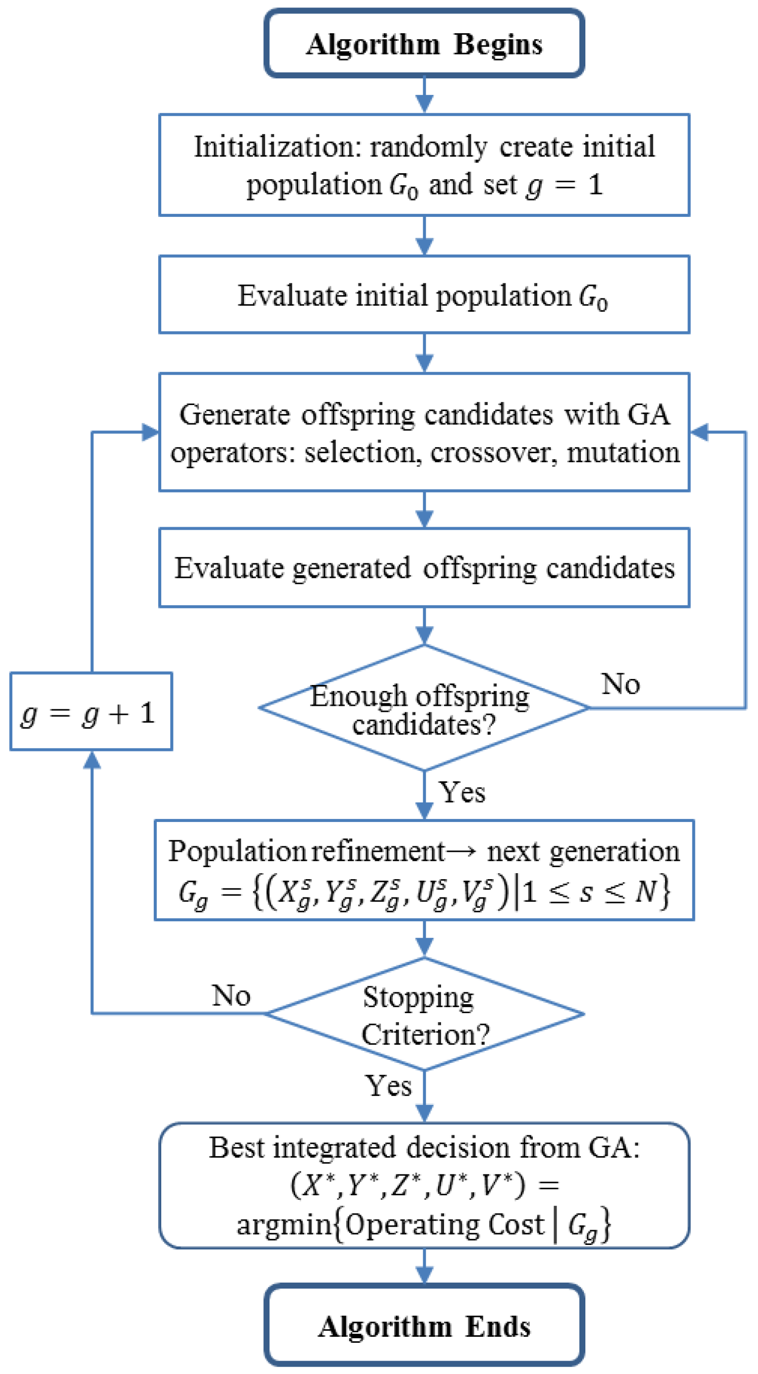
The optimization procedure pursued in this paper is based on the genetic algorithm (GA) paradigm [26]. Generally speaking, GA is a search heuristic that mimics the process of natural evolution. Each candidate solution, $\left(X,Y,Z,U,V\right)$, is represented by five chromosome portions, each of which is a decision vector relevant to the PM triggers, replenishment triggers, replenishment batch sizes, RM delivery speeds, and PM qualities, respectively (specifically, we have $X=\left(x_{1,1},x_{1,2}\dots ,x_{1,K_1},\dots ,x_{J,1},x_{J,2},\dots ,x_{J,K_J}\right)$, $Y=\left(y_1,y_2,\dots ,y_I\right)$, $Z=\left(z_1,z_2,\dots ,z_I\right)$, $U=\left(u_1,u_2,\dots ,u_J\right)$, and $V=\left(v_1,v_2,\dots ,v_J\right)$). The GA evolution starts from $N$ randomly generated candidate solutions as the initial population, labeled $G_0=\left\{\left(X_0^s,Y_0^s,Z_0^s,U_0^s,V_0^s\right)|1\le s\le N\right\}$. The fitness of each candidate solution in the population is taken to be inversely proportional to the expected operating cost of the system obtained via multiple simulation replications of system operations under the decision-making policy represented by that candidate solution. In order to generate offspring candidate solutions for the next generation, selection, crossover, and mutation operators are applied to the current generation. These operators are described below.

• Selection operator: A pair of parent solutions, namely $\left(X^{\alpha },Y^{\alpha },Z^{\alpha },U^{\alpha },V^{\alpha }\right)$ and $\left(X^{\beta },Y^{\beta },Z^{\beta },U^{\beta },V^{\beta }\right)$, are chosen from the current generation $g$ to mate and produce offspring candidate solutions for the next generation $g+1$, with a probability of selection being proportional to their fitness (in the GA literature, this is also known as fitness proportionate selection) [26].
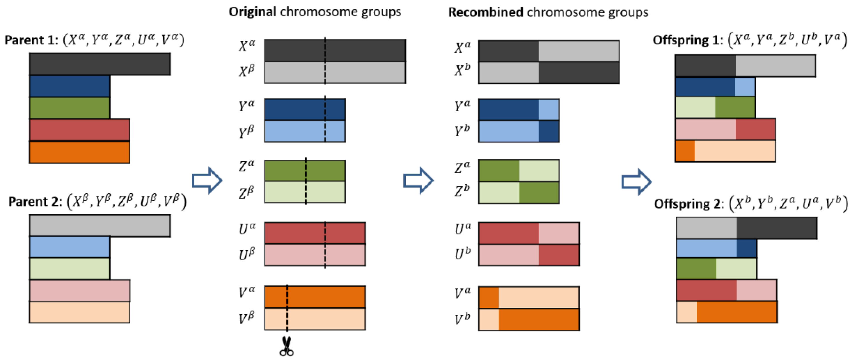
• Crossover operator: For a pair of selected parent solutions, a single-point crossover operator is executed at a random point in each of the five chromosome portions, leading to five pairs of recombined chromosome portions, namely, $\left\{X^a,X^b\right\}$, $\left\{Y^a,Y^b\right\}$, $\left\{Z^a,Z^b\right\}$, and $\left\{V^a,V^b\right\}$. Then, an offspring solution is generated via randomly selecting a chromosome portion from each of the five pairs, while the remaining chromosome portions forms another offspring solution. The above-described crossover operator is pictorially illustrated in Figure 2.
• Mutation operator: To promote genetic diversity in the offspring population, each gene in an offspring solution chromosome is selected with a small probability (commonly referred to as the mutation probability), and its value is perturbed to an adjacent candidate in its candidate value set. (For example, assume that the PM triggering usage level $x_{j,k}$ takes values in $X_{j,k}=\left\{35, 40, 45, 50\right\}$ and the current value for this gene is $x_{j,k}=40$. If the mutation operator is performed on this gene, the decision will mutate into either $x_{j,k}=35 \mathrm{or} 45$, with a small mutation probability.)

Following Muckstadt [26], N pairs of parent solutions are selected from the current generation, leading to the birth of 2N offspring solutions. If the top performing candidate solution in the parent generation has higher fitness than the 2N offspring candidates, it is added to the offspring population, thus enforcing the well-known concept of elitism in this GA [26]. From this set, the fittest N solutions are selected to form the next generation of candidate solutions.

Successive progression of generations yields ever-improving solutions, leading to lower expected operating cost of the system. The termination criterion for this algorithm is either a predetermined number of GA generations being reached, or the best candidate solution not being improved over a number of consecutive generations. The integrated decision-making policy is then taken to be the fittest candidate solution in the last GA generation, denoted by $\left(X^{\ast },Y^{\ast },Z^{\ast },U^{\ast },V^{\ast }\right)$.

Figure 3 illustrates the above-described algorithm.

4. Results

4.1. Baseline System and Restricted Systems

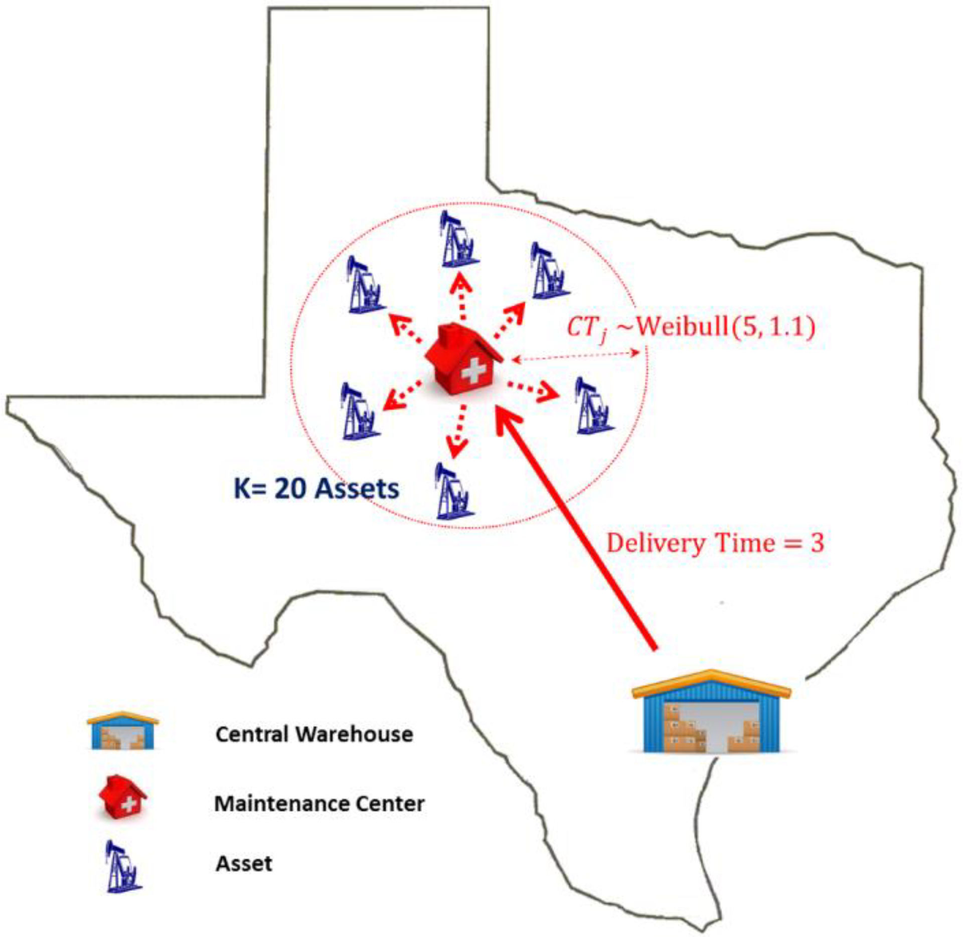
The newly proposed integrated decision-making policy described in Section 2 is evaluated in a series of simulations. For the baseline system, a central warehouse is connected to a maintenance center that provides maintenance service to 20 geographically dispersed assets, as illustrated in Figure 4. Altogether, 52 working parts are associated with the assets, and the corresponding spare parts (5 types of spare parts) need to be stocked in the maintenance facilities. Therefore, the integrated decision-making policy for the baseline system contains 102 decision variables, including 52 usage levels that trigger PM operations for the corresponding working parts, 5 re-order inventory levels and 5 replenishment batch sizes for managing spare part inventories in the maintenance center, 20 recovery rates that represent the quality of PM operations, and 20 acceleration rates that denote shipping options of the RM service. More details on the parameters of the baseline system can be found in Appendix A.

The decision-making planning horizon ($T$) is 365 × 5 time unis, and 100 replications of simulations are generated to estimate the unit-time operating cost for each candidate solution (this number of replications was selected in an ad hoc manner, by increasing the number of replications until their average effects did not change significantly with further increases). The simulation-based meta-heuristic algorithm described in Section 3 is repeated 10 times, with different randomly selected initial candidate solutions (i.e., 10 GA runs) to better explore the solution space [26]. In terms of computational costs, it always took less than 10 h to obtain a decision-making policy for this system on a relatively simple personal computer (Intel Core i5-3570 CPU, 16GB RAM, 64-bit Window 7). It should be noted that the simulation-based meta-heuristic optimization proposed in this paper is highly parallelizable (each candidate solution and each replication could be evaluated in parallel), and thus this algorithm could be greatly accelerated in a multi-processor environment [27].

The integrated decision-making policy proposed in this paper is derived under the assumption that multiple options exist for PM execution, RM transportation, and the size of replenishment orders. Special cases of the integrated decision-making policy can be obtained by restricting some of those options, and the indicators, ${\mathbb{I}}_1$, ${\mathbb{I}}_2$, and ${\mathbb{I}}_3$ will be used to denote such restrictions in the following manner:

(1)

${\mathbb{I}}_1=0$ denotes the existence of multiple PM operations with different quality levels, while ${\mathbb{I}}_1=1$ corresponds to the situation with perfect PM only. Thus, ${\mathbb{I}}_1=1$ implies fixing $v_j=1$ ($1\le j\le J$) in the formulation (1).

(2)

${\mathbb{I}}_2=0$ denotes the existence of multiple spare parts shipping options for RM, while ${\mathbb{I}}_2=1$ corresponds to normal RM delivery only. Thus, ${\mathbb{I}}_2=1$ implies fixing $u_j=0$ ($1\le j\le J$) in the Formulation (1).

(3)

${\mathbb{I}}_3=0$ denotes an (s, S) replenishment policy for spare parts inventory management in the maintenance center, while ${\mathbb{I}}_3=1$ indicates an (S − 1, S) replenishment policy in which only one spare part is shipped as a replenishment order. Thus, ${\mathbb{I}}_3=1$ implies fixing $z_i=1$ ($1\le i\le I$) in the Formulation (1).

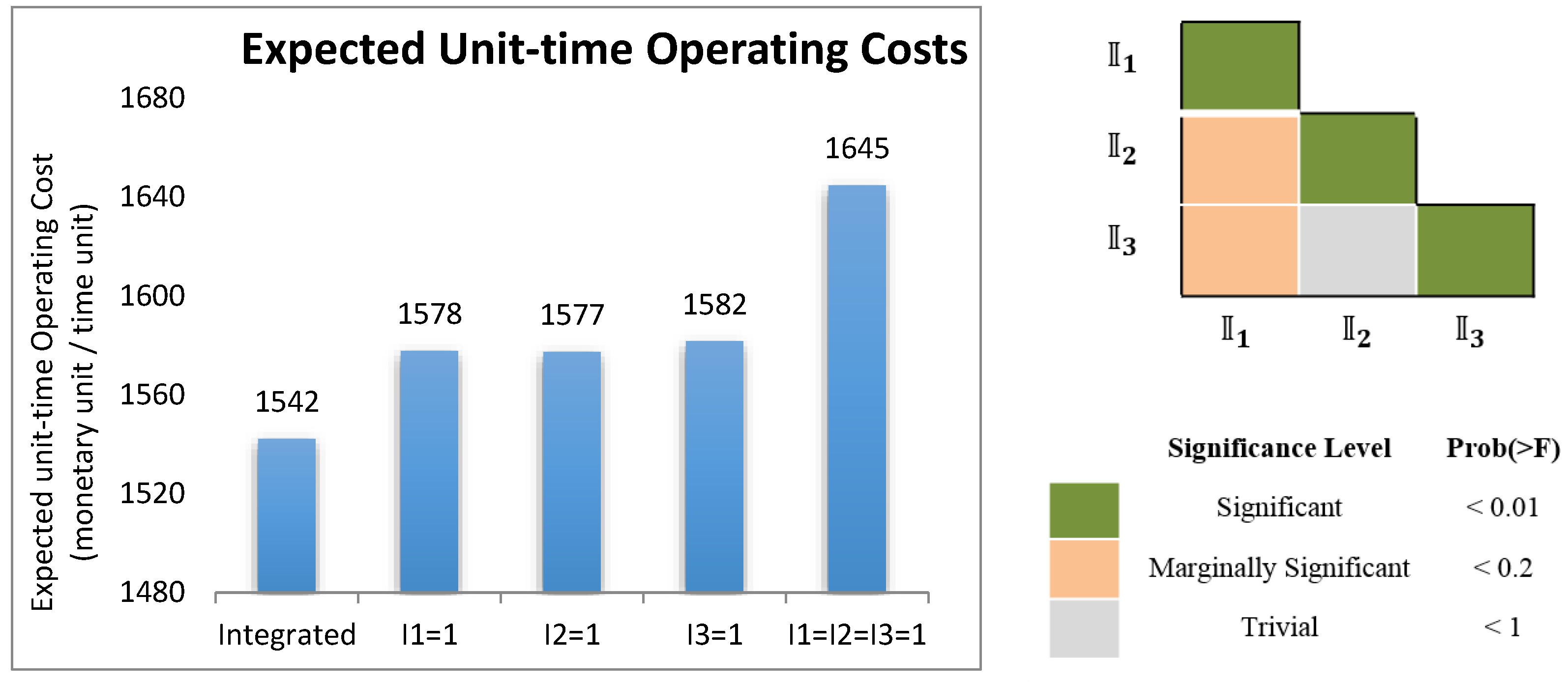
The benefits of considering multiple options for PM operations, RM deliveries, and replenishment size can be seen via the comparisons between the integrated decision-making policy and its special cases. As shown in Figure 5, a restriction on any of the three options leads to the increase in the system operating costs. Moreover, a two-way analysis of variance (ANOVA) model [28] is used to study the statistical effects of these multiple-choice options. In other words, factorial ANOVA is used to study effects of factors ${\mathbb{I}}_1$, ${\mathbb{I}}_2$, and ${\mathbb{I}}_3$ on the unit-time operating costs under the integrated decision-making policy. As is visible from Figure 5, the main effects of ${\mathbb{I}}_1$, ${\mathbb{I}}_2$, and ${\mathbb{I}}_3$ are all statistically significant, with a significance level of 0.01 or less, confirming the cost benefits of executing these multiple-choice options. Moreover, second order interaction effects of ${\mathbb{I}}_1\times {\mathbb{I}}_2$ and ${\mathbb{I}}_1\times {\mathbb{I}}_3$ are marginally significant, illustrating weak interactions between these factors (options).

A more detailed analysis of system performance under different decision-making options shows that when ${\mathbb{I}}_1=1$ and ${\mathbb{I}}_2={\mathbb{I}}_3=0$ (PM operations restricted to perfect PM only), the PM service becomes less efficient in terms of increased repair interventions (+93.3%) and higher cumulative PM costs (+71.7%). Furthermore, when ${\mathbb{I}}_2=1$ and ${\mathbb{I}}_1={\mathbb{I}}_3=0$, the prolonged RM delivery delays the lead to an 11.0% increase in asset downtimes. Finally, when ${\mathbb{I}}_3=1$ and ${\mathbb{I}}_1={\mathbb{I}}_2=0$ (inventory management policy restricted to the (S−1, S) replenishment policy), more replenishment deliveries are needed (+120.3%), leading to the increase in the replenishment delivery costs. Please note that a detailed list of statistics describing the system performance under the integrated decision-making policy for the baseline and restricted systems is provided in

Table A6. Performance statistics of the baseline system and the restricted systems in Section 4.1.

System Index	R0	R1	R2	R3	R4	R5	R6	Baseline
I1: Indicator for multi-mode PM option	1	0	1	1	0	0	1	0
I2: Indicator for RM expedition option	1	1	0	1	0	1	0	0
I3: Indicator for flexible replenishment option	1	1	1	0	1	0	0	0
System uptime (%)	94.40	94.91	95.29	94.54	95.71	94.85	95.18	95.66
Cumulative inventory holding times	12,493.95	15,910.15	15,911.44	16,226.56	16,036.76	17,208.50	16,258.20	16,288.49
Cumulative replenishment order	1311.20	1389.00	1388.72	614.71	1347.79	564.41	612.83	611.75
Cumulative number of PM orders	591.16	446.99	557.64	623.36	229.26	482.55	579.95	380.05
Cumulative number of RM orders	879.23	1012.68	903.93	859.42	1178.64	992.93	891.93	1084.70
Cumulative number of emergency orders	10.36	4.53	4.66	7.39	3.83	6.99	7.27	7.07
Unit-time fixed PM cost (monetary unit)	64.78	48.99	61.11	68.31	25.12	52.88	63.56	41.65
Unit-time added PM cost (monetary unit)	259.14	185.01	244.44	273.25	81.43	197.03	254.22	143.44
Unit-time RM cost (monetary unit)	481.77	554.89	495.30	470.92	645.83	544.07	488.73	594.36
Unit-time inventory holding cost (monetary unit)	68.46	87.18	87.19	88.91	87.87	94.29	89.09	89.25
Unit-time replenishment cost (monetary unit)	86.22	91.33	91.31	40.42	88.62	37.11	40.30	40.22
Unit-time downtime penalty (monetary unit)	673.98	643.59	546.06	659.11	510.60	645.00	556.99	516.64
Unit-time RM acceleration cost (monetary unit)	0.00	0.00	84.14	0.00	138.32	0.00	77.62	109.50
Unit-time emergency RM cost (monetary unit)	10.36	4.53	4.66	7.39	3.83	6.99	7.27	7.07

of Appendix A.

4.2. Sensitivity Analysis for Operating Costs under Integrated Policy

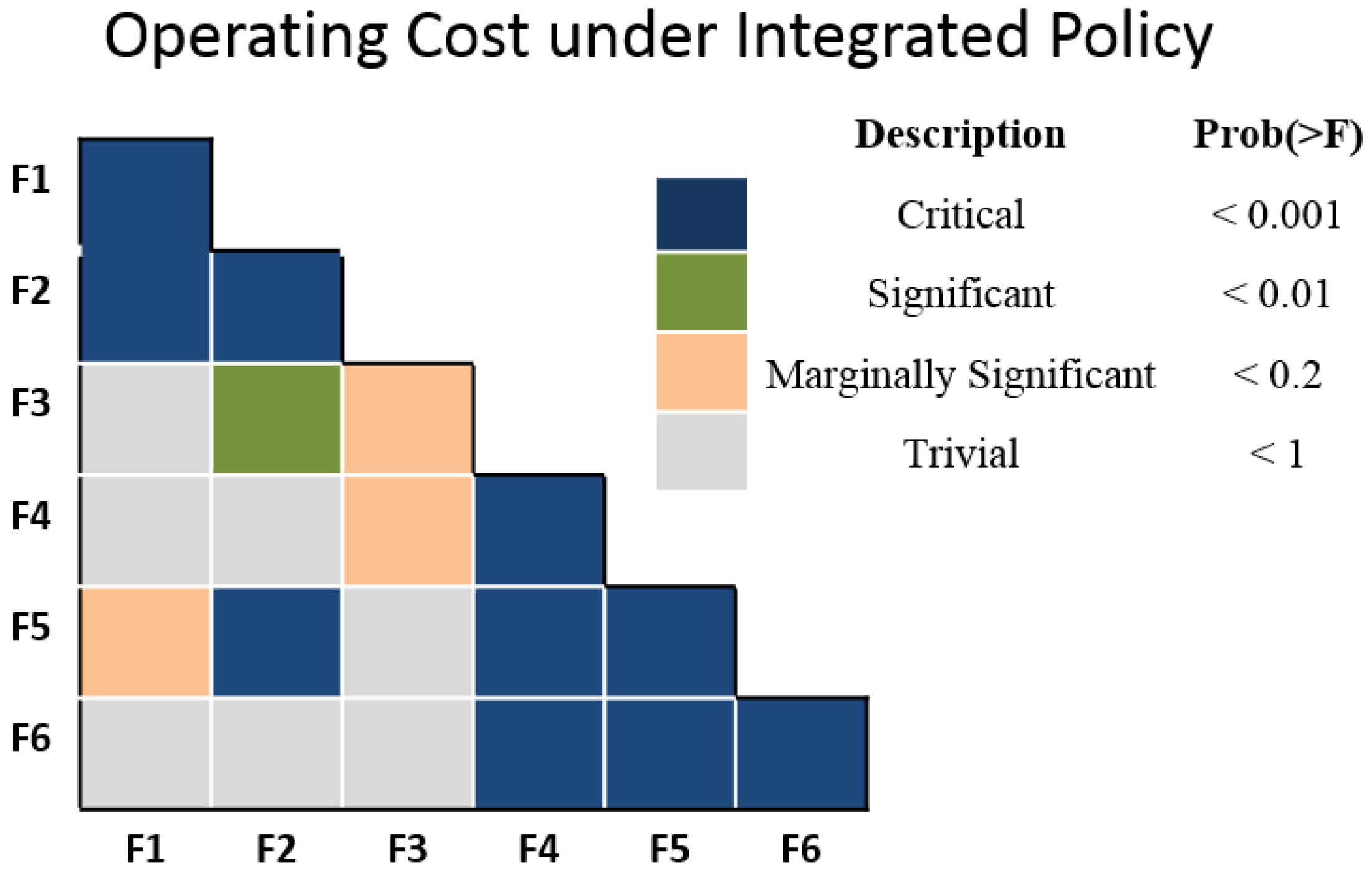
The ANOVA method can also be used to conduct sensitivity studies regarding various system parameters. In this section, the unit-time operating cost under the integrated decision-making policy is used as the response in a two-level factorial ANOVA, in which six input factors are considered. Specifically, factor F1 denotes the geographical dispersion level of the logistic network and factors F2–F6 are relevant to cost-related system parameters, denoting inventory holding cost per unit time, replenishment cost per order, PM quality improvement cost per order, penalty cost per unit downtime, and RM acceleration cost per order, respectively. Each factor is varied at two levels (low and high), resulting in 64 experimental levels in a $2^6$ DOE. More details on the DOE settings can be found in

Table A7. Factors F1–F6 used for the design-of-experiment (DOE) study in Section 4.2.

Factor	Description	Low vs. High Level	Relevant System Parameters Need to Be Scaled
F1	Geographical dispersion level	1.0 vs. 5.0	$CT$ and $\mathcal{C}{\mathcal{T}}_j(·)$ for $1\le j\le 20$
F2	Inventory holding cost per unit time	0.2 vs. 5.0	$H_i$ for $1\le i\le 5$
F3	Replenishment cost per order	1.0 vs. 5.0	$S_i^{fix}$ and $S_i^{add}$ for $1\le i\le 5$
F4	PM quality improvement cost per order	0.2 vs. 5.0	$M_{j,k}^{add}$ for $1\le j\le 20, 1\le k\le K_j$
F5	Penalty cost per unit downtime	0.2 vs. 5.0	$L_j$ for $1\le j\le 20$
F6	RM acceleration cost per order	0.2 vs. 5.0	$T_j$ for $1\le j\le 20$

and

Table A8. Operating costs under different system settings, with “L” denoting low level and “H” denoting high level.

	F1	F2	F3	F4	F5	F6	Cost		F1	F2	F3	F4	F5	F6	Cost		F1	F2	F3	F4	F5	F6	Cost
1	L	L	L	L	L	L	709.1	23	H	L	L	L	H	H	3244.8	45	L	H	L	H	H	L	1570.5
2	L	L	H	L	L	L	822.9	24	H	L	H	L	H	H	3095.0	46	L	H	H	H	H	L	3060.4
3	H	L	L	L	L	L	718.0	25	L	L	L	H	L	H	3237.3	47	H	H	L	H	H	L	3274.2
4	H	L	H	L	L	L	815.2	26	L	L	H	H	L	H	954.7	48	H	H	H	H	H	L	3581.8
5	L	L	L	L	H	L	2339.5	27	H	L	L	H	L	H	985.0	49	L	H	L	L	L	H	3791.0
6	L	L	H	L	H	L	2439.8	28	H	L	H	H	L	H	941.2	50	L	H	H	L	L	H	795.7
7	H	L	L	L	H	L	2383.2	29	L	L	L	H	H	H	998.3	51	H	H	L	L	L	H	1242.3
8	H	L	H	L	H	L	2451.1	30	L	L	H	H	H	H	4104.7	52	H	H	H	L	L	H	874.3
9	L	L	L	H	L	L	916.7	31	H	L	L	H	H	H	4162.4	53	L	H	L	L	H	H	1368.6
10	L	L	H	H	L	L	979.9	32	H	L	H	H	H	H	4167.9	54	L	H	H	L	H	H	3637.7
11	H	L	L	H	L	L	932.9	33	L	H	L	L	L	L	4183.9	55	H	H	L	L	H	H	3989.6
12	H	L	H	H	L	L	993.2	34	L	H	H	L	L	L	798.1	56	H	H	H	L	H	H	4151.8
13	L	L	L	H	H	L	2422.6	35	H	H	L	L	L	L	1241.3	57	L	H	L	H	L	H	4541.4
14	L	L	H	H	H	L	2495.5	36	H	H	H	L	L	L	927.4	58	L	H	H	H	L	H	1006.8
15	H	L	L	H	H	L	2461.2	37	L	H	L	L	H	L	1360.7	59	H	H	L	H	L	H	1329.7
16	H	L	H	H	H	L	2527.5	38	L	H	H	L	H	L	3046.8	60	H	H	H	H	L	H	1387.9
17	L	L	L	L	L	H	789.9	39	H	H	L	L	H	L	3237.6	61	L	H	L	H	H	H	1615.5
18	L	L	H	L	L	H	837.3	40	H	H	H	L	H	L	3465.2	62	L	H	H	H	H	H	4705.4
19	H	L	L	L	L	H	725.6	41	L	H	L	H	L	L	3768.8	63	H	H	L	H	H	H	4895.1
20	H	L	H	L	L	H	843.7	42	L	H	H	H	L	L	1010.1	64	H	H	H	H	H	H	5329.6
21	L	L	L	L	H	H	3024.1	43	H	H	L	H	L	L	1329.5
22	L	L	H	L	H	H	709.1	44	H	H	H	H	L	L	1353.4

of Appendix A.

In Figure 6, significance levels for the 6 main effects and 15 interaction effects are shown as the result of ANOVA. The main effects of the geographical dispersion level (F1) and four cost-related factors (F2, F4–F6), along with some of their interaction effects (F1 × F2, F2 × F5, F4 × F5, F4 × F6, F5 × F6), were found to be critical to the system operating cost. The criticality of these effects is plausible, as changes in these factors directly affect either the maintenance scheduling or spare parts logistic planning in the integrated decision-making policy.

Moreover, it is interesting to see that the replenishment cost per order (F3) is only marginally significant to the operating cost under the integrated decision-making policy, while its interaction effect with another inventory-related cost parameter, inventory holding cot per unit time (F2), is more significant than its main effect. This illustrates the fact that when only the replenishment costs become expensive, the negative effects can be partially offset through properly adjusting the inventory management policy, such as shipping more spare parts in a replenishment batch.

5. Conclusions and Future Work

In this paper, an integrated decision-making policy is proposed for concurrent preventive maintenance scheduling, spare parts inventory management and transportation planning in a system of geographically dispersed multi-part degrading assets and maintenance facilities that serve them. This integrated decision-making policy considers both perfect and imperfect maintenance options, as well as multiple shipping methods for spare part deliveries. This decision-making process was modeled as a stochastic optimization problem and was solved via a simulation-based optimization approach relying on a GA-based metaheuristic.

The integrated decision-making policy introduced in this paper was implemented in a series of simulations. The results illustrated statistically significant cost benefits of involving the options of multi-mode PM operations, expedited RM shipping, and flexible replenishment deliveries into the integrated decision-making process, while their interaction effects turned out to be only marginally significant according to a two-level ANOVA analysis. Furthermore, a DOE-based factorial analysis showed that operating costs under the integrated decision-making policy were sensitive to changes in geographical dispersion levels of the logistic network, as well as several maintenance/logistic cost parameters. Finally, the factorial analysis also illustrated that when only replenishment costs for spare parts become expensive, proper adjustment in inventory management under the integrated policy would allow the system to operate without a significant increase in operating costs.

Several possible avenues for possible future research can be identified. Firstly, the integrated decision-making process can be improved in the sense of robustness to uncertainties in the model parameters, which could be caused by limited availability of historical data or expert knowledge from which they need to be identified. Secondly, the assumptions of fixed network topology can be relaxed, leading to optimization of the maintenance facility locations and their interconnections with assets that need maintenance service. Finally, human resource planning also deserves further research, including optimization of the number, skills, and allocation of technicians needed to properly execute maintenance activities.

References

- Van Horenbeek, A.; Buré, J.; Cattrysse, D.; Pintelon, L.; Vansteenwegen, P. Joint maintenance and inventory optimization systems: A review. Int. J. Prod. Econ. 2013, 143, 499–508. [Google Scholar] [CrossRef]
- Zohrul Kabir, A.; Al-Olayan, A.S. Joint optimization of age replacement and continuous review spare provisioning policy. Int. J. Oper. Prod. Manag. 1994, 14, 53–69. [Google Scholar] [CrossRef]
- Kabir, A.Z.; Farrash, S. Simulation of an integrated age replacement and spare provisioning policy using SLAM. Reliab. Eng. Syst. Saf. 1996, 52, 129–138. [Google Scholar] [CrossRef]
- Sarker, R.; Haque, A. Optimization of maintenance and spare provisioning policy using simulation. Appl. Math. Model. 2000, 24, 751–760. [Google Scholar] [CrossRef]
- Hu, R.; Yue, C.; Xie, J. Joint optimization of age replacement and spare ordering policy based on genetic algorithm. In Proceedings of the International Conference on Computational Intelligence and Security (CIS’08), Suzhou, China, 13–17 December 2008; Volume 1, pp. 156–161. [Google Scholar]
- Acharya, D.; Nagabhushanam, G.; Alam, S. Jointly optimal block-replacement and spare provisioning policy. IEEE Trans. Reliab. 1986, 35, 447–451. [Google Scholar] [CrossRef]
- Jiang, Y.; Chen, M.; Zhou, D. Joint optimization of preventive maintenance and inventory policies for multi-unit systems subject to deteriorating spare part inventory. J. Manuf. Syst. 2015, 35, 191–205. [Google Scholar] [CrossRef]
- Brezavšček, A.; Hudoklin, A. Joint optimization of block-replacement and periodic-review spare-provisioning policy. IEEE Trans. Reliab. 2003, 52, 112–117. [Google Scholar] [CrossRef]
- Van Horenbeek, A.; Scarf, P.A.; Cavalcante, C.A.; Pintelon, L. The effect of maintenance quality on spare parts inventory for a fleet of assets. IEEE Trans. Reliab. 2013, 62, 596–607. [Google Scholar] [CrossRef]
- Ilgin, M.A.; Tunali, S. Joint optimization of spare parts inventory and maintenance policies using genetic algorithms. Int. J. Adv. Manuf. Technol. 2007, 34, 594–604. [Google Scholar] [CrossRef]
- Huang, R.; Meng, L.; Xi, L.; Liu, C.R. Modeling and analyzing a joint optimization policy of block-replacement and spare inventory with random-leadtime. IEEE Trans. Reliab. 2008, 57, 113–124. [Google Scholar] [CrossRef]
- Panagiotidou, S. Joint optimization of spare parts ordering and maintenance policies for multiple identical items subject to silent failures. Eur. J. Oper. Res. 2014, 235, 300–314. [Google Scholar] [CrossRef]
- Bjarnason, E.T.S.; Taghipour, S. Optimizing simultaneously inspection interval and inventory levels (s, S) for a k-out-of-n system. In Proceedings of the 2014 Annual, Reliability and Maintainability Symposium (RAMS), Colorado Springs, CO, USA, 27–30 January 2014; pp. 1–6. [Google Scholar]
- Bjarnason, E.T.S.; Taghipour, S. Periodic Inspection Frequency and Inventory Policies for a k-out-of-n System. IIE Trans. 2015, 48, 638–650. [Google Scholar] [CrossRef]
- Alrabghi, A.; Tiwari, A.; Alabdulkarim, A. Simulation based optimization of joint maintenance and inventory for multi-components manufacturing systems. In Proceedings of the 2013 Winter Simulation Conference (WSC), Washington, DC, USA, 8–11 December 2013; pp. 1109–1119. [Google Scholar]
- Lynch, P.; Adendorff, K.; Yadavalli, V.; Adetunji, O. Optimal spares and preventive maintenance frequencies for constrained industrial systems. Comput. Ind. Eng. 2013, 65, 378–387. [Google Scholar] [CrossRef]
- Wang, W. A stochastic model for joint spare parts inventory and planned maintenance optimisation. Eur. J. Oper. Res. 2012, 216, 127–139. [Google Scholar] [CrossRef]
- Wang, W.; Syntetos, A.A. Spare parts demand: Linking forecasting to equipment maintenance. Transp. Res. Part E Logist. Transp. Rev. 2011, 47, 1194–1209. [Google Scholar] [CrossRef]
- Nguyen, D.; Bagajewicz, M. Optimization of preventive maintenance in chemical process plants. Ind. Eng. Chem. Res. 2010, 49, 4329–4339. [Google Scholar] [CrossRef]
- Nguyen, D.Q.; Brammer, C.; Bagajewicz, M. New tool for the evaluation of the scheduling of preventive maintenance for chemical process plants. Ind. Eng. Chem. Res. 2008, 47, 1910–1924. [Google Scholar] [CrossRef]
- Chen, M.-C.; Hsu, C.-M.; Chen, S.-W. Optimizing joint maintenance and stock provisioning policy for a multi-echelon spare part logistics network. J. Chin. Inst. Ind. Eng. 2006, 23, 289–302. [Google Scholar] [CrossRef]
- Beyer, H.-G.; Sendhoff, B. Robust optimization–a comprehensive survey. Comput. Methods Appl. Mech. Eng. 2007, 196, 3190–3218. [Google Scholar] [CrossRef]
- Mahadevan, S.; Rebba, R. Inclusion of model errors in reliability-based optimization. J. Mech. Des. 2006, 128, 936–944. [Google Scholar] [CrossRef]
- Zitrou, A.; Bedford, T.; Daneshkhah, A. Robustness of maintenance decisions: Uncertainty modelling and value of information. Reliab. Eng. Syst. Saf. 2013, 120, 60–71. [Google Scholar] [CrossRef]
- Muckstadt, J.A. Analysis and Algorithms for Service Parts Supply Chains; Springer Science & Business Media: Berlin/Heidelberg, Germany, 2005. [Google Scholar]
- Sivanandam, S.; Deepa, S. Introduction to Genetic Algorithms; Springer Science & Business Media: Berlin/Heidelberg, Germany, 2007. [Google Scholar]
- Cantú-Paz, E. Efficient and Accurate Parallel Genetic Algorithms; Kluwer Academic Publishers: Norwell, MA, USA, 2001. [Google Scholar]
- Montgomery, D.C. Design and Analysis of Experiments; John Wiley & Sons: Hoboken, NJ, USA, 2017. [Google Scholar]
Figure 1.
Spare part logistic network considered in this paper. Illustration of the three-level logistic network (left-hand side) and illustration of spare part inventory flows (right-hand side). PM—Preventive Maintenance; RM—Reactive Maintenance.
Figure 2.
A realization of the crossover operator on two parent candidate solutions.
Figure 3.
Flow chart of the genetic algorithm (GA)-based optimization pursued in this paper.
Figure 4.
Illustration of the spare part logistic network for the baseline system.
Figure 5.
Comparison of unit time operating costs for the baseline and restricted systems (left-hand side), as well as a result of analysis of variance (ANOVA) of the unit time operating costs, with significance levels for the effects of factors , , and (right-hand side).
Figure 6.
ANOVA analysis of the unit time operating costs under the integrated policy, with significance levels for the main/interaction effects of F1–F6.