Tether Space Mobility Device Attitude Control during Tether Extension and Winding

Abstract

Recently, advancements in space technology have opened up more opportunities for human beings to work in outer space. It is expected that upsizing of manned space facilities, such as the International Space Station, will further this trend. Therefore, a unique means of transportation is necessary to ensure that human beings can move about effectively in microgravity environments. In the present study, we propose a tether-based mobility system, which moves the user by winding a tether attached to a structure at the destination. However, there is a problem in that the attitude of the user becomes unstable during winding of the tether. Therefore, a Tether Space Mobility Device (TSMD) attitude control method for winding a tether is examined through numerical analysis. The proposed analytical model consists of one flexible body and three rigid bodies. The contact force between the tether and the inlet is considered. We verified the validity of the proposed model through experiments. Furthermore, we proposed a TSMD attitude control method during tether winding while focusing on changes in the system’s rotational kinetic energy. Using the proposed analytical model, the angular velocity of a rigid body system is confirmed to converge to 0 deg/s when control is applied.

1. Introduction

As space developments have advanced, opportunities for human beings to work in outer space have increased. Upsizing of manned space facilities, such as the International Space Station, is expected to further this trend. Since the interior of these manned facilities can be presumed to have the same microgravity conditions as the external environment, in order for human beings to perform efficiently, a unique means of transportation that takes these conditions into consideration is necessary. In addition, while it is conceivable that thrusters, or something similar, could be used to move objects, such devices cannot be used within the enclosed living environment of a space station because they would pollute the air.

Based on this background, a number of attempts have been made to develop a highly compact and lightweight tether system for use as an actuator under microgravity conditions [1]. For example, Nohmi et al. developed a satellite system for use in a microgravity environment that was based on extension and contraction of a tether, and confirmed the utility of their system through a space demonstration experiment [2]. In addition, a propulsion method based on the Lorentz effect, which uses a conductive tether to interfere with geomagnetism, has also been proposed, and research on its control method has been conducted [3]. Also, many tethered deorbiting missions have been proposed, and there are also many proposals for dynamic models [4,5]. In addition, a tether-net space robot system utilizing a net shaped tether has also been proposed [6].

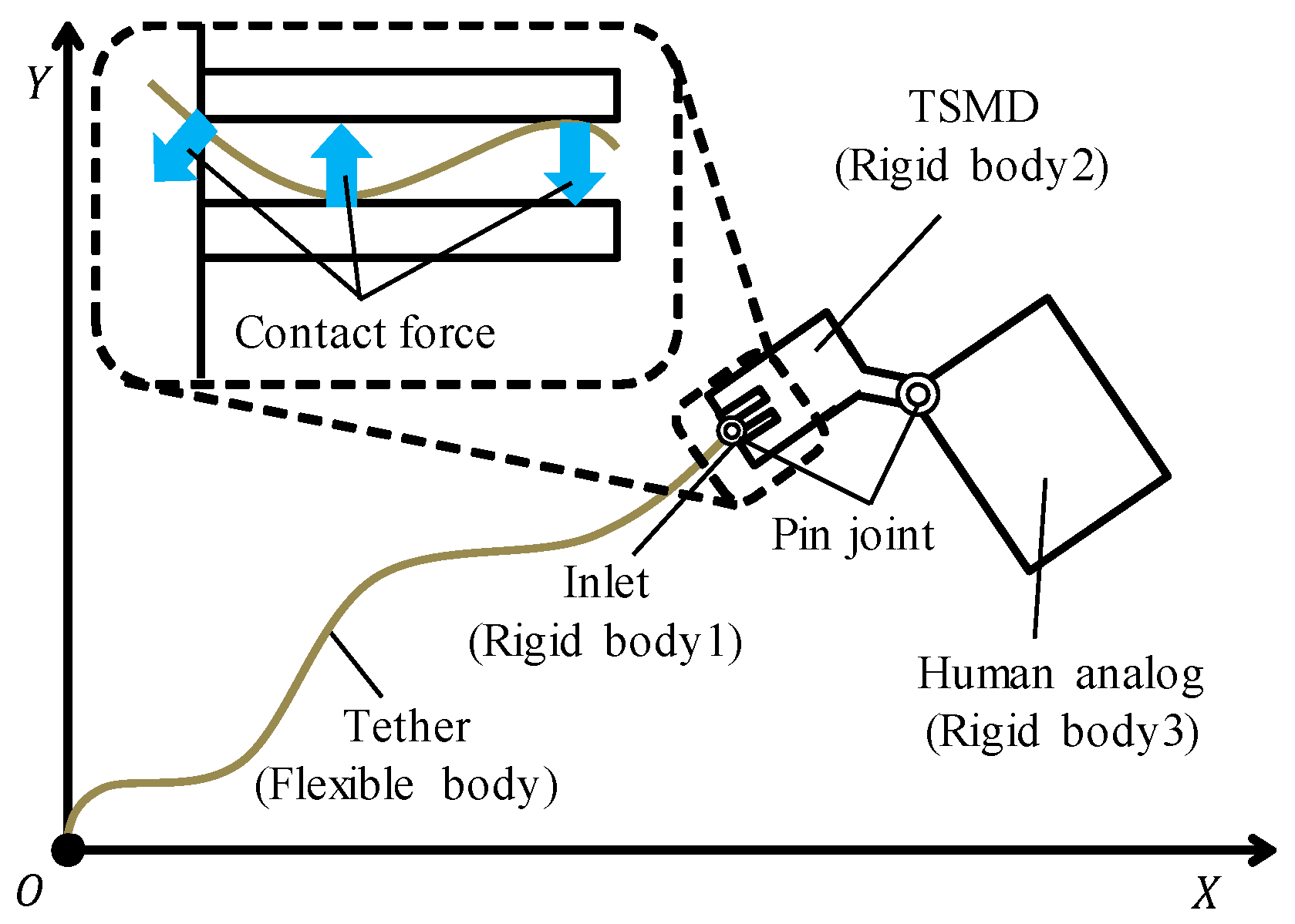
In the present paper, the authors propose a Tether Space Mobility Device (TSMD) as a means of facilitating human mobility within a manned facility under microgravity conditions [7]. The basic concept of the TSMD is shown in Figure 1. When the operator fires the TSMD toward his/her destination, the tether shoots out from the device, and the end of the tether secures itself to the target point. The tether is then wound into the TSMD by a motor, thereby pulling the human operator toward his or her desired destination.

However, since the tension acting on the tether under microgravity conditions will be very small, it is assumed that large deformations and displacements will occur when the tether is extended and wound, which means that the attitude of the TSMD operator has the potential to become unstable. Therefore, in the present paper, we report on the construction of an analytical model for simulating the movement of the TSMD during tether extension and winding operations. Then, after confirming the validity of the analytical model through comparisons with the experimental results simulating a microgravity environment, we propose a tether winding speed control method that stabilizes the attitude of the TSMD operator using the system’s rotational kinetic energy.

2. TSMD Modeling and Formulation

2.1. Analytical Model

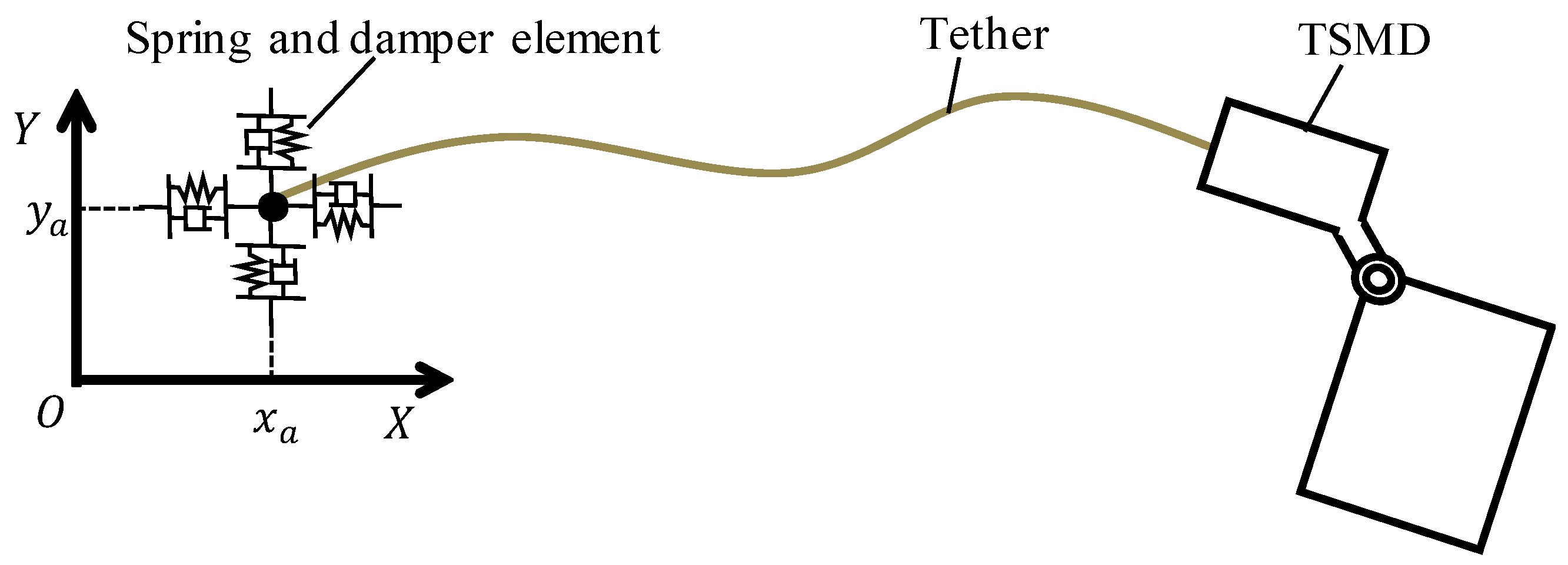
Figure 2 shows the analytical model of the TSMD. This model can simulate a series of movements involving extending and winding the tether. In this model, the tether is made of a flexible body, and the rigid bodies are composed of three components: an inlet, the TSMD, and a human analog simulating the user of TSMD. The inlet is located inside the TSMD, but since there is the possibility of mounting an actuator in the future, the inlet is considered as an independent rigid body. The flexible body is formulated by absolute nodal coordinate formulation (ANCF), which was suggested by Shabana et al. to express motion with large deformation and large displacement [8]. The rigid bodies are formulated by augmented formulation, which is a method of multibody dynamics. Extension and winding operations are represented by driving the constraint between the element node at the rear end of the tether and rigid body 2. The interaction between the rigid bodies and the flexible body can be investigated in this model. The interaction occurs according to the reaction force and the tether tension. The reaction force is calculated when the flexible body contacts the edge and the inner surface of rigid body 1.

2.2. Flexible Body Formulation

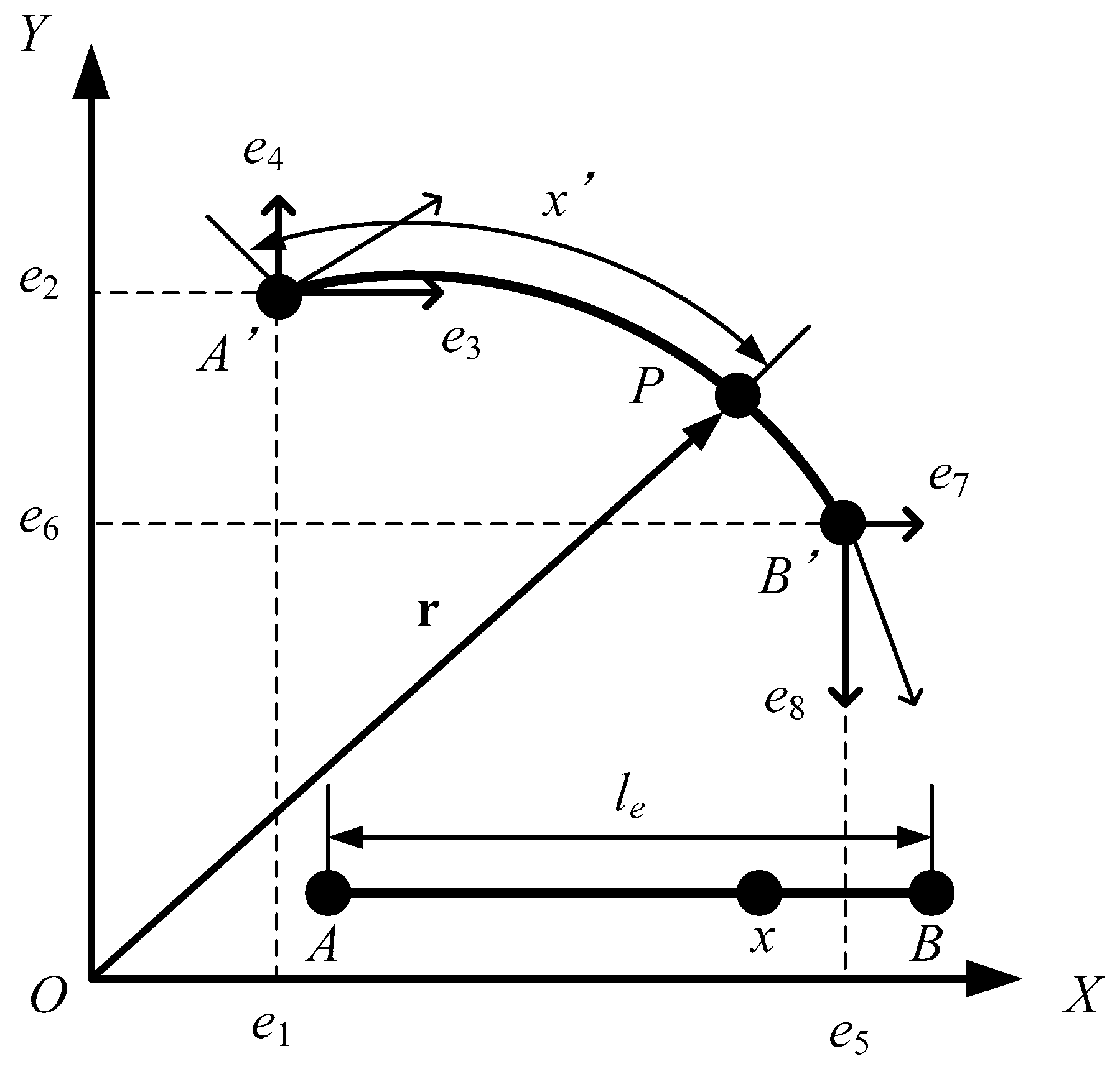
In this model, the motion of the flexible body is formulated using the absolute nodal coordinate formulation (ANCF) proposed by Shabana et al. The beam elements placed in the global coordinate system $O$-$XY$ are shown in Figure 3. The element before deformation is defined as $OA$, and the element after deformation is defined as $O^{\prime }{A}^{\prime }$. The position vector $r$ of an arbitrary point $P$ on an element can be expressed as follows using a shape function $S$ and a node coordinate vector e:

$$\mathbf{r}=\mathbf{S}\mathbf{e}$$

(1)

where the node coordinate vector e is composed of flexible body elements:

$$\mathbf{e}={\left[\begin{array}{cccccccc}{e}_1& e_2& e_3& e_4& e_5& e_6& e_7& e_8\end{array}\right]}^T$$

(2)

where (e₁,e₂) and (e₅,e₆) represent the XY coordinates of the node at the element end. Similarly, (e₃,e₄) and (e₇,e₈) represent the spatial derivative in the XY coordinate system of the node at each element end. Furthermore, the shape function $S$ is determined based on the assumption of a Bernoulli-Eulerian beam, as follows:

$$\mathbf{S}={\left[\begin{array}{cc}1-3{\xi }^2+2{\xi }^3& 0\\ 0& 1-3{\xi }^2+2{\xi }^3\\ l_e\left(\xi -2{\xi }^2+{\xi }^3\right)& 0\\ 0& l_e\left(\xi -2{\xi }^2+{\xi }^3\right)\\ 3{\xi }^2-2{\xi }^3& 0\\ 0& 3{\xi }^2-2{\xi }^3\\ l_e\left({\xi }^3-{\xi }^2\right)& 0\\ 0& l_e\left({\xi }^3-{\xi }^2\right)\end{array}\right]}^T$$

(3)

where $l_e$ is the length of the beam element, and we assume that $x$ is the position of arbitrary point $P$ from element node $O$ before deformation, so that $\xi =x/l_e$. The kinetic energy T of this beam element is expressed by the following equation:

$$T=\frac{1}{2}{{\displaystyle \int }}_V\rho {\dot{\mathbf{r}}}^T\dot{\mathbf{r}}dV=\frac{1}{2}{\dot{\mathbf{e}}}^T\left({{\displaystyle \int }}_V\rho {\mathbf{S}}^T\mathbf{S}dV\right)\dot{\mathbf{e}}$$

(4)

where $\rho$ is the density of the beam element. Then, the mass matrix ${\mathbf{M}}_{\mathit{t}}$ of the beam element is given by the following equation:

$${\mathbf{M}}_{\mathit{t}}={{\displaystyle \int }}_V\rho {\mathbf{S}}^T\mathbf{S}dV$$

(5)

Next, the elastic force of the beam element is derived. Several methods have been proposed for modeling the elastic force. In this report, we use model T1 proposed by Berzeri et al. [9]. In addition, we use the bending elastic force and the model S L1 proposed by Wago et al. [10]. The strain energy $U_t$ for bending deformation of a beam element is expressed by the following equation:

$$U_t=\frac{1}{2}{{\displaystyle \int }}_0^{l_e}{E}_{t}I{\kappa }^{2}dx$$

(6)

where $E_t$ is the elastic modulus in the bending direction, $I$ is the geometrical moment of inertia, and $\kappa$ is the curvature. Assuming that the axial deformation of the beam element is minute, the square of $\kappa$ can be expressed by the following equation:

$${\kappa }^2\approx {\left|\frac{d^2\mathbf{r}}{d{x}^2}\right|}^2={\mathbf{e}}^T{\left(\frac{d^2\mathbf{S}}{d{x}^2}\right)}^T\left(\frac{d^2\mathbf{S}}{d{x}^2}\right)\mathbf{e}$$

(7)

Substituting Equation (7) into Equation (6), the strain energy for bending deformation is given by the following equation:

$$U_t=\frac{1}{2}{\mathit{e}}^T\left\{{{\displaystyle \int }}_0^{l_e}{E}_{t}I{\left(\frac{d^2\mathit{S}}{d{x}^2}\right)}^T\left(\frac{d^2\mathit{S}}{d{x}^2}\right)dx\right\}\mathit{e}$$

(8)

The bending elastic force vector ${\mathbf{Q}}_t$ is obtained by partially differentiating $U_t$ with respect to $e$ and is expressed by the following equation:

$${\mathbf{Q}}_t={\left(\frac{\partial U_t}{\partial \mathbf{e}}\right)}^T={\mathbf{K}}_t\mathbf{e}$$

(9)

where ${\mathbf{K}}_t$ is a flexural rigidity matrix and is expressed by the following equation:

$${\mathbf{K}}_t={{\displaystyle \int }}_0^{l_e}{E}_{t}I{\left(\frac{d^2\mathbf{S}}{d{x}^2}\right)}^T\left(\frac{d^2\mathbf{S}}{d{x}^2}\right)dx$$

(10)

Finally, the elastic force in the axial direction is derived. The axial strain energy $U_l$ of the beam element is expressed by the following equation:

$$U_l=\frac{1}{2}{{\displaystyle \int }}_0^{l_e}{E}_{l}A{\epsilon }^{2}dx$$

(11)

where $E_l$ is the elastic modulus in the axial direction, $A$ is the cross-sectional area, and $\epsilon$ is the strain in the axial direction, which can be expressed by the following equation using the Green-Lagrange strain tensor:

$$\epsilon =\frac{1}{2}\left\{{\left(\frac{d\mathit{r}}{dx}\right)}^T\left(\frac{d\mathit{r}}{dx}\right)-1\right\}=\frac{1}{2}\left\{{\mathit{e}}^T{\left(\frac{d\mathit{S}}{dx}\right)}^T\left(\frac{d\mathit{S}}{dx}\right)\mathit{e}-1\right\}$$

(12)

When $\epsilon$ is partially differentiated with respect to $e$, the following equation is obtained:

$${\left(\frac{\partial \epsilon }{\partial \mathbf{e}}\right)}^T={\left(\frac{d\mathbf{S}}{dx}\right)}^T\left(\frac{d\mathbf{S}}{dx}\right)\mathbf{e}$$

(13)

The axial elastic force vector ${\mathbf{Q}}_l$ is obtained by partially differentiating $U_l$ with respect to e and is expressed by the following equation:

$${\mathbf{Q}}_l={\left(\frac{\partial U_l}{\partial \mathbf{e}}\right)}^T=\left\{{{\displaystyle \int }}_0^{l_e}{E}_{l}A\epsilon {\left(\frac{d\mathbf{S}}{dx}\right)}^T\left(\frac{d\mathbf{S}}{dx}\right)dx\right\}\mathbf{e}={\mathbf{K}}_l\mathbf{e}$$

(14)

where ${\mathbf{K}}_l$ is a nonlinear axial stiffness matrix. When $\epsilon$ in Equation (14) is replaced with the average axial strain $\overline{\epsilon }$, ${\mathbf{K}}_l$ is expressed by the following equation:

$${\mathbf{K}}_l=\overline{\epsilon }{{\displaystyle \int }}_0^{l_e}{E}_{l}A{\left(\frac{d\mathbf{S}}{dx}\right)}^T\left(\frac{d\mathbf{S}}{dx}\right)dx$$

(15)

The length of the beam element along the neutral axis after deformation is defined as $l_s$, which can be expressed by the following equation [10]:

$$l_s=\frac{1}{2}\left[{\mathbf{e}}^T\left\{{{\displaystyle \int }}_0^{l_e}{\left(\frac{d\mathbf{S}}{dx}\right)}^T\left(\frac{d\mathbf{S}}{dx}\right)dx\right\}\mathbf{e}+l_e\right]$$

(16)

Define the average axial strain of the beam element as follows using the length change along the neutral axis after deformation $\left(l_s-l_e\right)$:

$${\overline{\epsilon }}_{S\_L1}=\frac{l_s-l_e}{l_e}$$

(17)

Substituting Equation (17) into Equation (15), ${\mathbf{K}}_l$ is expressed by the following equation:

$${\mathbf{K}}_l={\overline{\epsilon }}_{S\_L1}{{\displaystyle \int }}_0^{l_e}{E}_{l}A{\left(\frac{d\mathbf{S}}{dx}\right)}^T\left(\frac{d\mathbf{S}}{dx}\right)dx$$

(18)

When the external force term including gravity is ${\mathbf{Q}}_f$, the motion equation of the beam element finally becomes as follows:

$${\mathbf{M}}_{\mathit{t}}\ddot{\mathbf{e}}+\left({\mathbf{K}}_t+{\mathbf{K}}_l\right)\mathbf{e}={\mathbf{Q}}_f$$

(19)

2.3. Rigid Body Formulation

The rigid body formulation is based on an augmented formulation. In this model, the rigid body system is composed of three rigid bodies. The equation of motion for the rigid bodies is:

$${\mathbf{M}}_r{\ddot{\mathbf{q}}}_r={\mathbf{Q}}_r$$

(20)

where

$$\begin{gathered} {\mathbf{M}}_r=diag\left(m_{r1}, m_{r1}, I_{r1}, m_{r2}, m_{r2}, I_{r2}, m_{r3}, m_{r3}, I_{r3}\right) \\ {\mathbf{q}}_r={\left[\begin{array}{ccccccccc}{x}_{r1}& y_{r1}& {\theta }_{r1}& x_{r2}& y_{r2}& {\theta }_{r2}& x_{r3}& y_{r3}& {\theta }_{r3}\end{array}\right]}^T \\ {\mathbf{Q}}_r={\left[\begin{array}{ccccccccc}{F}_{r1x}& F_{r1y}& M_{r1}& F_{r2x}& F_{r2y}& M_{r2}& F_{r3x}& F_{r3y}& M_{r3}\end{array}\right]}^T \end{gathered}$$

(21)

and where $m_{rj}$ are the masses of the rigid bodies, $I_{rj}$ are their moments of inertia $\left(j=1,2,3\right)$, $x_{rj},y_{rj}$ represent the centers of the rigid bodies, ${\theta }_{rj}$ are their rotation angles $\left(j=1,2,3\right)$, and $F_{rjx},F_{rjy},\mathrm{and}{M}_{rj}$ are the external forces and moments of the rigid bodies, respectively. Thus, the equation of motion for the system is:

$$\mathbf{M}\ddot{\mathbf{q}}=\mathbf{Q}$$

(22)

where

$$\begin{gathered} \mathbf{M}=\left[\begin{array}{cc}{\mathbf{M}}_{\mathit{t}}& \mathbf{0}\\ \mathbf{0}& {\mathbf{M}}_{\mathit{r}}\end{array}\right] \\ \mathbf{q}={\left[\begin{array}{cc}{\mathbf{e}}^{\mathit{T}}& {\mathbf{q}}_{\mathit{r}}{}^{\mathit{T}}\end{array}\right]}^{\mathit{T}} \\ \mathbf{Q}={\left[\begin{array}{cc}{\mathbf{Q}}_{\mathit{f}}-{\mathbf{Q}}_{\mathit{t}}-{\mathbf{Q}}_{\mathit{l}}& {\mathbf{Q}}_{\mathit{r}}\end{array}\right]}^{\mathit{T}} \end{gathered}$$

(23)

Next, we formulate the system constraints. Pin joints connect rigid bodies 1 and 2, and rigid bodies 2 and 3. Then, the system constraints are given by:

$$\left[\begin{array}{c}{\mathbf{R}}_1+{\mathbf{T}}_1{\overline{\mathbf{u}}}_2^1-{\mathbf{R}}_2-{\mathbf{T}}_2{\overline{\mathbf{u}}}_1^2\\ {\mathbf{R}}_2+{\mathbf{T}}_2{\overline{\mathbf{u}}}_3^2-{\mathbf{R}}_3-{\mathbf{T}}_3{\overline{\mathbf{u}}}_2^3\end{array}\right]=\mathbf{0}$$

(24)

where ${\mathbf{R}}_j$ is the position vector of the center of rigid body $j$ in absolute coordinates, ${\mathbf{T}}_j$ is transformation matrix from the local coordinate system to the absolute coordinate system, and ${\overline{\mathbf{u}}}_j^i$ is a position vector up to the joint point of rigid body $j$ in local coordinates. Then, the relative angle between the rigid bodies is determined by the driving constraints and is described as:

$$\left[\begin{array}{c}{\theta }_{r1}-{\theta }_{r2}-{\theta }_{r12}\left(t\right)\\ {\theta }_{r2}-{\theta }_{r3}-{\theta }_{r23}\left(t\right)\end{array}\right]=\mathbf{0}$$

(25)

where ${\theta }_{r12}\left(t\right)$ is the relative angle between rigid bodies 1 and 2, and ${\theta }_{r23}\left(t\right)$ is the relative angle between rigid bodies 2 and 3.

In the present paper, we do not consider the relative motion between the rigid bodies, and set the relative angles between rigid bodies as ${\theta }_{r12}\left(t\right)={\theta }_{r23}\left(t\right)=0$. Extension and winding of the tether is expressed by displacing the node at the end of the tether at velocity V in the X direction in the object coordinate system of rigid body 2. Therefore, if the total length of the tether is $l_0$, the node constraint at the end of the tether and rigid body 2 can be described as:

$$\left[\begin{array}{c}{e}_5{}^{\left(n\right)}\\ e_6{}^{\left(n\right)}\end{array}\right]-{\mathbf{R}}_2-{\mathbf{T}}_2\left({\overline{\mathbf{u}}}_1^2+\left[\begin{array}{c}{{\displaystyle \int }}_o^{t}Vdt+l_0\\ 0\end{array}\right]\right)=\mathbf{0}$$

(26)

Therefore, the constraint equations for the system $\mathsf{\Phi }$ can be written as:

$$\mathsf{\Phi }=\left[\begin{array}{c}\left[\begin{array}{c}{e}_5{}^{\left(n\right)}\\ e_6{}^{\left(n\right)}\end{array}\right]-{\mathbf{R}}_2-{\mathbf{T}}_2\left({\overline{\mathbf{u}}}_1^2+\left[\begin{array}{c}{{\displaystyle \int }}_o^{t}Vdt+l_0\\ 0\end{array}\right]\right)\\ {\mathbf{R}}_1+{\mathbf{T}}_1{\overline{\mathbf{u}}}_2^1-{\mathbf{R}}_2-{\mathbf{T}}_2{\overline{\mathbf{u}}}_1^2\\ {\mathbf{R}}_2+{\mathbf{T}}_2{\overline{\mathbf{u}}}_3^2-{\mathbf{R}}_3-{\mathbf{T}}_3{\overline{\mathbf{u}}}_2^3\\ {\theta }_{r1}-{\theta }_{r2}-{\theta }_{r12}\left(t\right)\\ {\theta }_{r2}-{\theta }_{r3}-{\theta }_{r23}\left(t\right)\end{array}\right]=\mathbf{0}$$

(27)

The differential algebraic equations are obtained as:

$$\left[\begin{array}{cc}\mathbf{M}& {\mathsf{\Phi }}_{\mathbf{q}}{}^T\\ {\mathsf{\Phi }}_{\mathbf{q}}& \mathbf{0}\end{array}\right]\left[\begin{array}{c}\ddot{\mathbf{q}}\\ \mathsf{\lambda }\end{array}\right]=\left[\begin{array}{c}\mathbf{Q}\\ \mathsf{\gamma }\end{array}\right]$$

(28)

where ${\mathsf{\Phi }}_{\mathbf{q}}$ is the Jacobean matrix, $\mathsf{\lambda }$ are Lagrange multipliers, and $\mathsf{\gamma }$ is the acceleration equation. Differentiating the constraint twice with respect to time, we obtain:

$$\mathsf{\gamma }=-{\left({\mathsf{\Phi }}_{\mathbf{q}}\dot{\mathbf{q}}\right)}_{\mathbf{q}}\dot{\mathbf{q}}-2{\mathsf{\Phi }}_{\mathbf{q}t}\dot{\mathbf{q}}-{\mathsf{\Phi }}_{tt}$$

(29)

2.4. Rigid Body Formulation

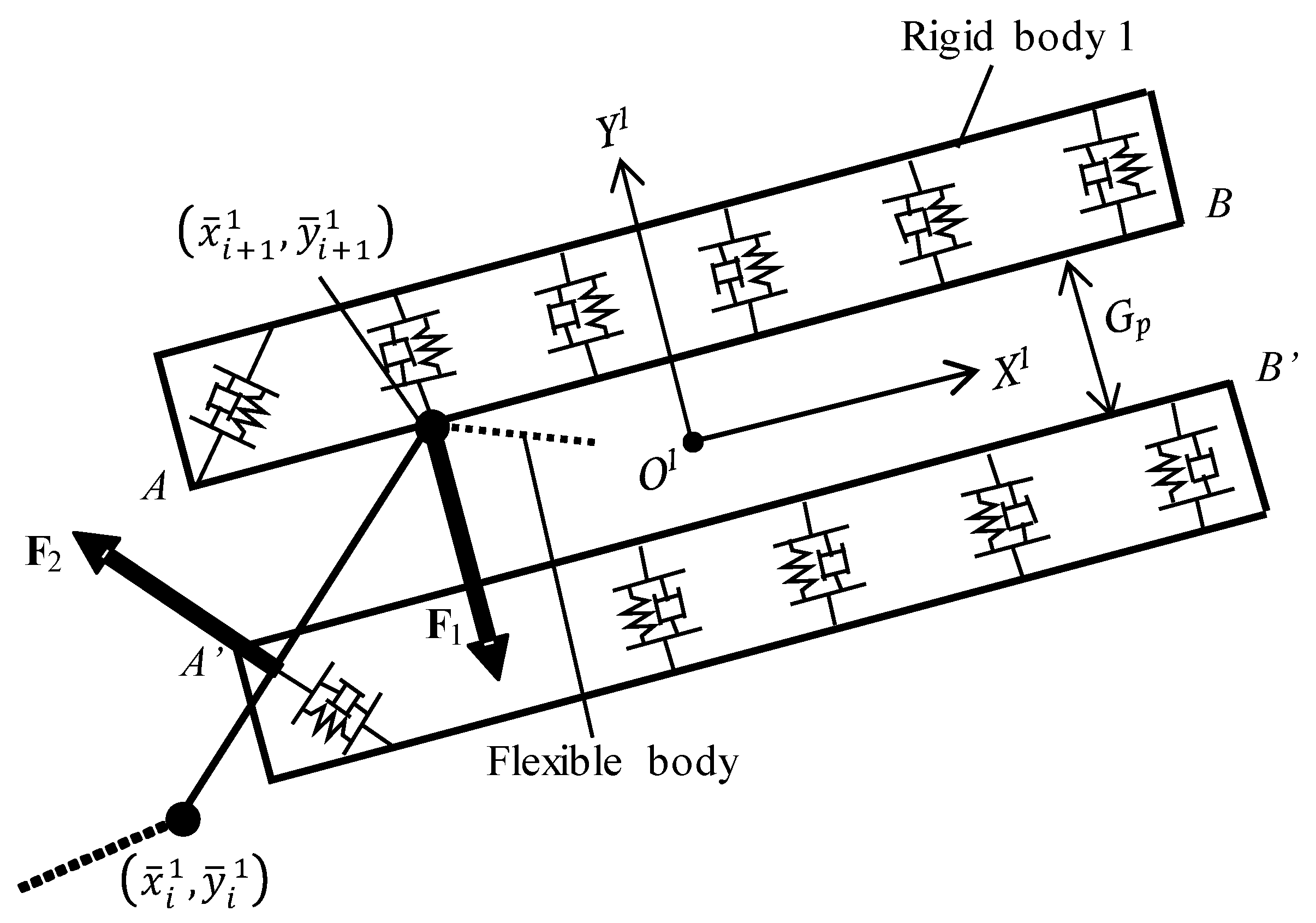
Next, we present the formulation for contact force from the rigid body system on the tether. The contact force between the flexible and rigid bodies is calculated by a spring and a damper element. In addition, we consider the contact force to be divided into ${\mathbf{F}}_1$ and ${\mathbf{F}}_2$ in order to express the suction phenomenon near the suction port. Here, ${\mathbf{F}}_1$ is the reaction force caused by the inner wall of rigid body 1 in a situation in which the node of the beam element is retracted completely, and ${\mathbf{F}}_2$ is the reaction force at the edge of rigid body 1 when the node of the beam element is being retracted. First, the force ${\mathbf{F}}_1$ from the elastic wall inside the rigid body is considered.

Figure 4 shows the beam element retracted into rigid body 1. The number of the node located outside of and closest to the tip of rigid body 1 is set to $i$, whereas the number of the node located inside of and closest to the tip of rigid body 1 is set to $i+1$. Assuming that the position vector in the global coordinate system for the $i+1$th node is $\left(x_{i+1},y_{i+1}\right)$ and the position vector in the object coordinate system for rigid body 1 is $\left({\overline{x}}_{i+1}^1,{\overline{y}}_{i+1}^1\right)$, the following equation is obtained:

$$\left[\begin{array}{c}{\overline{x}}_{i+1}^1\\ {\overline{y}}_{i+1}^1\end{array}\right]={\mathbf{T}}_1^{-1}\left(\left[\begin{array}{c}{x}_{i+1}\\ y_{i+1}\end{array}\right]-{\mathbf{R}}_1\right)$$

(30)

Therefore, taking into consideration the frictional force acting between the beam element and the rigid body, the force ${\mathbf{F}}_1$ from the inner wall AB of rigid body 1 on the $i+1$th node can be expressed in the overall coordinate system as follows:

$$\begin{array}{ll}{\mathbf{F}}_1={\mathbf{T}}_1\left[\begin{array}{c}-{\mu }_1\left[-k_1\left\{{\overline{y}}_{i+1}^1-\mathrm{sgn}\left({\overline{y}}_{i+1}^1\right)\frac{G_p}{2}\right\}-c_1{\dot{\overline{y}}}_{i+1}^1\right]\\ -k_1\left\{{\overline{y}}_{i+1}^1-\mathrm{sgn}\left({\overline{y}}_{i+1}^1\right)\frac{G_p}{2}\right\}-c_1{\dot{\overline{y}}}_{i+1}^1\end{array}\right]& \left(\left|{\overline{y}}_{i+1}^1\right|\ge \frac{G_p}{2}\right)\\ {\mathbf{F}}_1=\mathbf{0}& \left(\left|{\overline{y}}_{i+1}^1\right|<\frac{G_p}{2}\right)\hfill \end{array}$$

(31)

where $k_1$ and $c_1$ are the spring constant and the damping coefficient for the elastic wall in rigid body 1, while taking contact rigidity into account. The force ${\mathbf{F}}_{1r}$ and moment $M_{1r}$ acting on rigid body 1, which are resultant forces of the reaction force of elements in rigid body 1, are described as

$$\left[\begin{array}{c}{\mathbf{F}}_{1r}\\ M_{1r}\end{array}\right]=\left[\begin{array}{c}\sum \left(-{\mathbf{F}}_1\right)\\ \sum \left(-{\overline{x}}_{i+1}^1{\overline{F}}_{1y}^1+{\overline{y}}_{i+1}^1{\overline{F}}_{1x}^1\right)\end{array}\right]$$

(32)

where ${\overline{F}}_{1x}^1$ and ${\overline{F}}_{1y}^1$ are the X and Y direction components when ${\mathbf{F}}_1$ is expressed in the object coordinate system of rigid body 1.

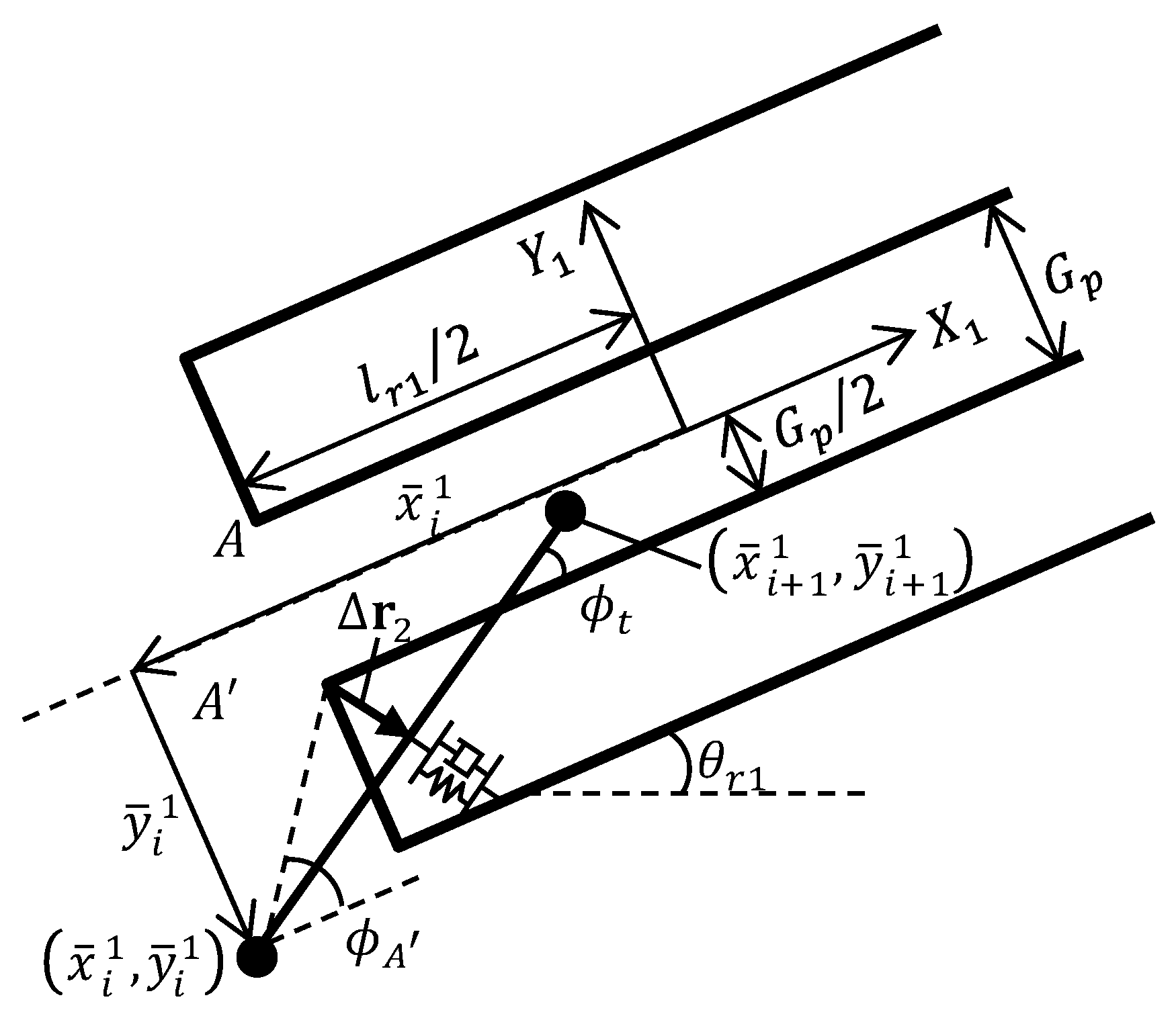
Next, we consider the reaction force ${\mathbf{F}}_2$ at the edge of rigid body 1. Figure 5 shows the flexible body element that is drawn into rigid body 1. For simplicity, it is assumed that the retracted beam element is not geometrically deformed. Assuming that the deformation of the object coordinate system of rigid body1 is $\Delta {\overline{\mathbf{r}}}_2^1$, the contact force ${\overline{\mathbf{F}}}_{k2}^1$ of the edge of rigid body 1 in the object coordinate system can be expressed as follows:

$${\overline{\mathbf{F}}}_{k2}^1=\left[\begin{array}{c}{\overline{F}}_{k2x}^1\\ {\overline{F}}_{k2y}^1\end{array}\right]=-k_2\Delta {\overline{\mathbf{r}}}_2^1-c_2\Delta {\dot{\overline{\mathbf{r}}}}_2^1$$

(33)

where $k_2$ and $c_2$ are the spring constant and the damping coefficient, respectively, for the elastic wall in the vicinity of the tip of rigid body 1, considering the contact rigidity. Assuming that the angle of the beam element in the object coordinate system of rigid body 1 is ${\varphi }_t$ and the angle of the line segment formed by the $i$th node and the suction port tip $A^{\prime }\left(A\right)$ is ${\varphi }_{A^{\prime }}\left({\varphi }_A\right)$, the condition that the tip of the beam element and the tip of rigid body 1 contact each other is described as:

$$\{\begin{array}{cc}{\varphi }_t\le {\varphi }_A& \left({\overline{y}}_i^1\ge \frac{G_p}{2}\right)\\ {\varphi }_t\le {\varphi }_{A^{\prime }}& \left({\overline{y}}_i^1\le -\frac{G_p}{2}\right)\end{array}$$

(34)

Then, ${\varphi }_t$, ${\varphi }_A$, and ${\varphi }_{A^{\prime }}$ are given by:

$${\varphi }_t=\left|{\tan }^{-1}\left(\frac{{\overline{y}}_{i+1}^1-{\overline{y}}_i^1}{{\overline{x}}_{i+1}^1-{\overline{x}}_i^1}\right)\right|, {\varphi }_A=\left|{\tan }^{-1}\left(\frac{\frac{G_p}{2}-{\overline{y}}_i^1}{-\frac{l_{r1}}{2}-{\overline{x}}_i^1}\right)\right|, {\varphi }_{A^{\prime }}=\left|{\tan }^{-1}\left(\frac{-\frac{G_p}{2}-{\overline{y}}_i^1}{-\frac{l_{r1}}{2}-{\overline{x}}_i^1}\right)\right|$$

(35)

When the beam element satisfies the boundary conditions in Equation (34), the magnitude of $\Delta {\overline{\mathbf{r}}}_2^1$ is:

$$\begin{array}{ll}\left|\Delta {\overline{\mathbf{r}}}_2^1\right|=\left\{{\overline{y}}_i^1+\left({\overline{x}}_i^1+\frac{l_{r1}}{2}\right)\tan {\varphi }_t-\frac{G_p}{2}\right\}\cos {\varphi }_t\hfill & \left({\varphi }_t\le {\varphi }_A\right)\hfill \\ \left|\Delta {\overline{\mathbf{r}}}_2^1\right|=\left\{-{\overline{y}}_i^1+\left({\overline{x}}_i^1+\frac{l_{r1}}{2}\right)\tan {\varphi }_t-\frac{G_p}{2}\right\}\cos {\varphi }_t\hfill & \left({\varphi }_t\le {\varphi }_{A^{\prime }}\right)\hfill \end{array}$$

(36)

and when $\left|\Delta {\overline{\mathbf{r}}}_2^1\right|$ is decomposed in the $X$ and $Y$ directions in the object coordinate system, we obtain:

$$\begin{array}{ll}\Delta {\overline{\mathbf{r}}}_2^1=\left\{{\overline{y}}_i^1+\left({\overline{x}}_i^1+\frac{l_{r1}}{2}\right)\tan {\varphi }_t-\frac{G_p}{2}\right\}\left[\begin{array}{c}\frac{\sin 2{\varphi }_t}{2}\\ \frac{\cos 2{\varphi }_t+1}{2}\end{array}\right]\hfill & \left({\varphi }_t\le {\varphi }_A\right)\hfill \\ \Delta {\overline{\mathbf{r}}}_2^1=\left\{-{\overline{y}}_i^1+\left({\overline{x}}_i^1+\frac{l_{r1}}{2}\right)\tan {\varphi }_t-\frac{G_p}{2}\right\}\left[\begin{array}{c}\frac{\sin 2{\varphi }_t}{2}\\ -\frac{\cos 2{\varphi }_t+1}{2}\end{array}\right]\hfill & \left({\varphi }_t\le {\varphi }_{A^{\prime }}\right)\hfill \end{array}$$

(37)

Next, we consider the frictional force from the edge of rigid body 1 on the beam element. The frictional force in the object coordinate system from the tip of rigid body 1 on the beam element ${\overline{\mathbf{F}}}_{f2}^1$ is described as:

$${\overline{\mathbf{F}}}_{f2}^1={\mu }_2\left[\begin{array}{c}-\mathrm{sgn}\left({\dot{{\overline{x}}_i}}^1\right)|{\overline{F}}_{k2y}^1|\\ -\mathrm{sgn}\left({\dot{{\overline{y}}_i}}^1\right)|{\overline{F}}_{k2x}^1|\end{array}\right]$$

(38)

where ${\mu }_2$ is the friction coefficient between the beam element and the tip of rigid body 1. Therefore, the force from the tip of rigid body 1 on the beam element in the global coordinate system is:

$${\mathbf{F}}_2=\left[\begin{array}{c}{F}_{2x}\\ F_{2y}\end{array}\right]={\mathbf{T}}_1\left({\overline{\mathbf{F}}}_{k2}^1+{\overline{\mathbf{F}}}_{f2}^1\right)$$

(39)

Since the force determined by Equation (39) is the force from the beam element, this force is decomposed into components ${\mathbf{F}}_{ei}$ and ${\mathbf{F}}_{ei+1}$, which are received by the nodes at each end of the beam element. Assuming that ${\mathbf{F}}_2/l_e$ acts uniformly on the beam elements, ${\mathbf{F}}_{ei}$ and ${\mathbf{F}}_{ei+1}$ are expressed by the following equation based on the principle of virtual work:

$$\left[\begin{array}{c}{\mathbf{F}}_{ei}\\ {\mathbf{F}}_{ei+1}\end{array}\right]={\left[\begin{array}{cccccccc}\frac{1}{2}{F}_{2x}& \frac{1}{2}{F}_{2y}& \frac{l_e}{12}{F}_{2x}& \frac{l_e}{12}{F}_{2y}& \frac{1}{2}{F}_{2x}& \frac{1}{2}{F}_{2y}& -\frac{l_e}{12}{F}_{2x}& -\frac{l_e}{12}{F}_{2y}\end{array}\right]}^T$$

(40)

The force ${\mathbf{F}}_{2r}$ and the rotational moment $M_{2r}$ from the beam element on rigid body 1 by contact are described as:

$$\begin{array}{cc}\left[\begin{array}{c}{\mathbf{F}}_{2r}\\ M_{2r}\end{array}\right]=\left[\begin{array}{c}-{\mathbf{F}}_2\\ \frac{l_{r1}}{2}{\overline{F}}_{2y}^1+\frac{G_p}{2}{\overline{F}}_{2x}^1\end{array}\right]& \left({\varphi }_t\le {\varphi }_A\right)\\ \left[\begin{array}{c}{\mathbf{F}}_{2r}\\ M_{2r}\end{array}\right]=\left[\begin{array}{c}-{\mathbf{F}}_2\\ \frac{l_{r1}}{2}{\overline{F}}_{2y}^1-\frac{G_p}{2}{\overline{F}}_{2x}^1\end{array}\right]& \left({\varphi }_t\le {\varphi }_{A^{\prime }}\right)\end{array}$$

(41)

where ${\overline{F}}_{2x}^1$ and ${\overline{F}}_{2y}^1$ are the X and Y direction components, and ${\mathbf{F}}_2$ is expressed in the object coordinate system for rigid body 1. For $k_1$ and $k_2$, we herein assume that the deformation of the elastic wall is small, and they are given a large value so that the retracted beam element does not extend outside of rigid body 1. When considering the stability of the analysis, $c_1$ and $c_2$ provide critical attenuation for the system formed by the beam elements and $k_1$ and $k_2$. The contact force from rigid body 2 on the beam element can be obtained by replacing the object coordinate system of rigid body 1 with rigid body 2, and then setting $G_p=0$, where it is assumed that the beam element retracted into rigid body 2 is treated as recovered, and no reaction force is applied to rigid body 2.

2.5. Extending and Attaching the Tether

Figure 6 shows the analytical model representing the adsorption of the tether tip. As shown in Figure 6, a point mass m1 (kg) is attached to the tip of the tether. An initial velocity is given to the point mass by a spring force for injection, and the tether is extended. At this time, the force acting on the point mass is also given to the rigid body as a reaction force. Here, let $y_a$ be the y coordinate $e_2$ of the tether tip when the x coordinate $e_1$ of the tether tip reaches the suction position $x_a$. When the point mass reaches $x_a$, as shown in Figure 6, the point mass is fixed by the spring element and the damper element, thereby simulating the adsorption of the tether tip. Adsorption forces $F_{ax}$ and $F_{ay}$ acting on the tether tip are expressed by the following equation:

$$\begin{gathered} F_{ax}=-k_a\left(e_1-x_a\right)-c_a{\dot{e}}_1 \\ {F}_{ay}=-k_a\left(e_2-y_a\right)-c_a{\dot{e}}_2 \end{gathered}$$

(42)

where $k_a$ is a spring constant, and $c_a$ is a damping coefficient. Equation (42) is applied to the external force term 1st, 2nd row on the right-hand side of Equation (28), so that it acts on the element node at the tip of the tether.

In order to prevent deceleration of the tether tip during extension of the tether, a constant deflection amount is generated by setting the constraint condition formula according to the speed of the tether tip. The value of V in the constraint conditional expression of Equation (26) is set as follows:

$$V={\dot{e_1}}^{\left(1\right)}+K_e\left(l_{et}-l_s\right)$$

(43)

where $e_i{}^{\left(j\right)}$ is the nodal coordinate of the $j$th element, $K_e$ is the proportional gain, $l_{et}$ is the target deflection in the extending tether, and $l_s$ is the length of the tether that is not collected in the rigid body.

3. Validity of the Analytical Model

3.1. Experimental Setup

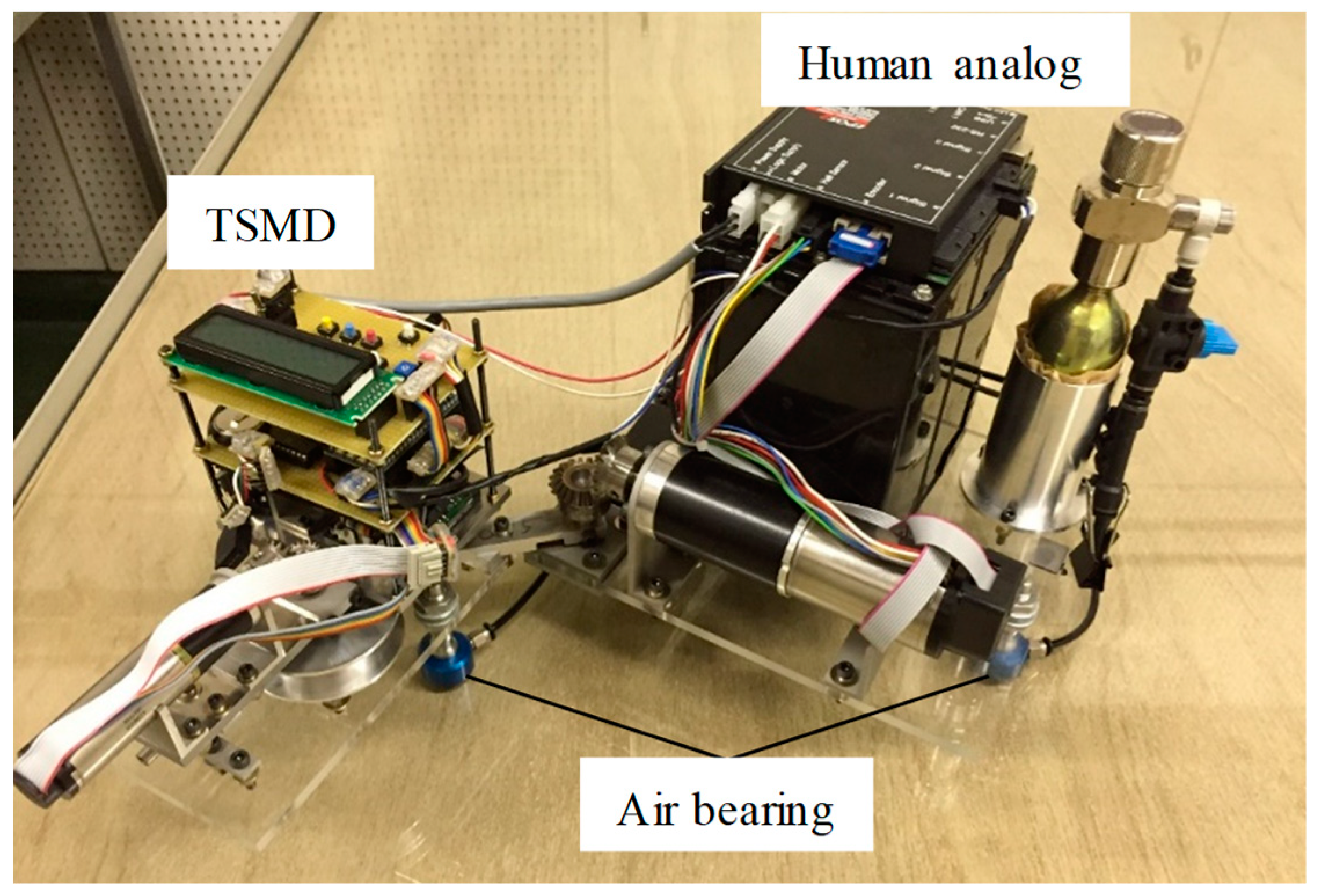
The experimental equipment (shown in Figure 7) is described in this section. This experimental equipment consists of the TSMD and a unit for simulating the influence of the weight of a human body. A method using air bearings, which are widely used in space robot control experiments [11], was adopted to simulate a two-dimensional (2D) microgravity environment. The TSMD is equipped with a reel for winding the tether, a brushless direct current (DC) motor and a microcomputer (mbed NXP_LPC1768, 96 MHZ). The human analog is equipped with a battery. Since the mass of the battery shifts the system’s center of gravity (COG), tension-based rotation occurs easily. In addition, the human analog is equipped with a nine-axis motion sensor that allows its movements to be measured precisely and a motor for disturbance input. The experiment was carried out on a flat table made from a smooth glass plate (1.5 m × 3 m).

3.2. Analytical Model

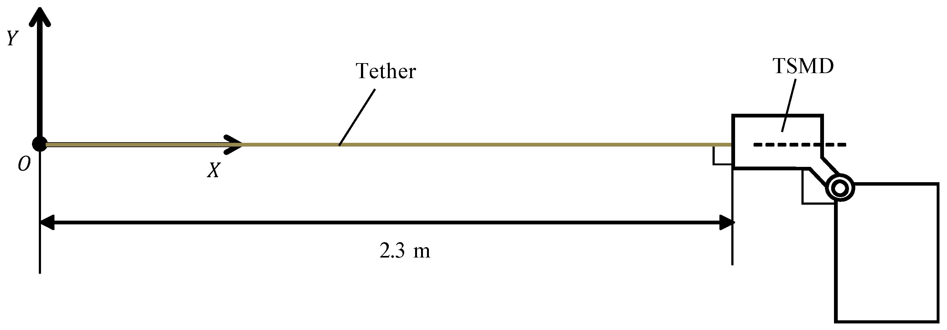
In order to confirm the validity of the proposed analytical model, we focused on tether behavior during winding, and compared the results of numerical simulations and experiments. Figure 8 shows the initial conditions used. The arm of the TSMD and the human analog are not driven, but rather are fixed so as to be perpendicular to the TSMD, as shown in Figure 8. The tether was stretched from the TSMD via the arm, and the tether tip was fixed in place at the origin point. The experimental equipment was arranged so that the tether and the TSMD are aligned along the X axis. The tether winding then began and rotation of the experimental equipment during the winding movement was verified. This experiment was repeated three times at the same speed.

Table 1. Experimental equipment conditions.

Total length of the tether $l$ (m)	2.355
Diameter of the tether $d$ (m)	5.2 × 10−4
Density of the tether $\rho$ (kg/m3)	1.140
Transverse elastic modulus $E_t$ (GPa)	1.93
Longitudinal elastic modulus $E_l$ (GPa)	1.93
Element number of the tether	70
Mass of the arm $M_{r1}$ (kg)	0.0367
Mass of the TSMD $M_{r2}$ (kg)	0.817
Mass of the human analog $M_{r3}$ (kg)	7.78
Moment of inertia of the arm $I_{r1}$ (kg·m2)	9.4 × 10−6
Moment of inertia of the TSMD $I_{r2}$ (kg·m2)	2.6 × 10−3
Moment of inertia of the human analog $I_{r3}$ (kg·m2)	0.0548
Length of the arm $l_{r1}$ (m)	0.055
Length of the TSMD (m)	0.17
Length of the human analog (m)	0.19
Width of the arm (m)	0.006
Width of the TSMD (m)	0.095
Width of the human analog (m)	0.22
Gap of the arm $G_p$ (m)	3.0 × 10−3
Spring constant of the inside wall of the arm $k_1$ (N/m)	230
Spring constant of the edge of the arm $k_2$ (N/m)	230
Damping coefficient of the inside wall of the arm $c_1$ (N/(m/s))	0.0866
Damping coefficient of the inside wall of the arm $c_2$ (N/(m/s))	0.0866
Coefficient of friction of the inside wall of the arm ${\mu }_1$	0.1
Coefficient of friction of the edge of the arm ${\mu }_2$	0.1

shows the parameters used in the experiment. The measurement time was set to 6 s. For numerical simulation, a workstation (Intel^® Core^TM i7-4790K CPU 4.00 GHz) is used.

3.3. Winding the Tether at Constant Speed

In the present paper, we consider winding the tether at a constant speed to validate the analysis model. Hereinafter, this condition will be referred to as constant speed winding. Under this condition, the reel is accelerated at a constant acceleration until the target winding speed is reached from the stationary state. When the winding speed reaches the target speed, the tether is thereafter taken up at a constant speed. In the present paper, the target winding speed is set to 0.1 m/s, and the acceleration is determined to be 0.256 m/s² from the motor characteristics obtained in advance.

3.4. Comparison of Analytical and Experimental Results

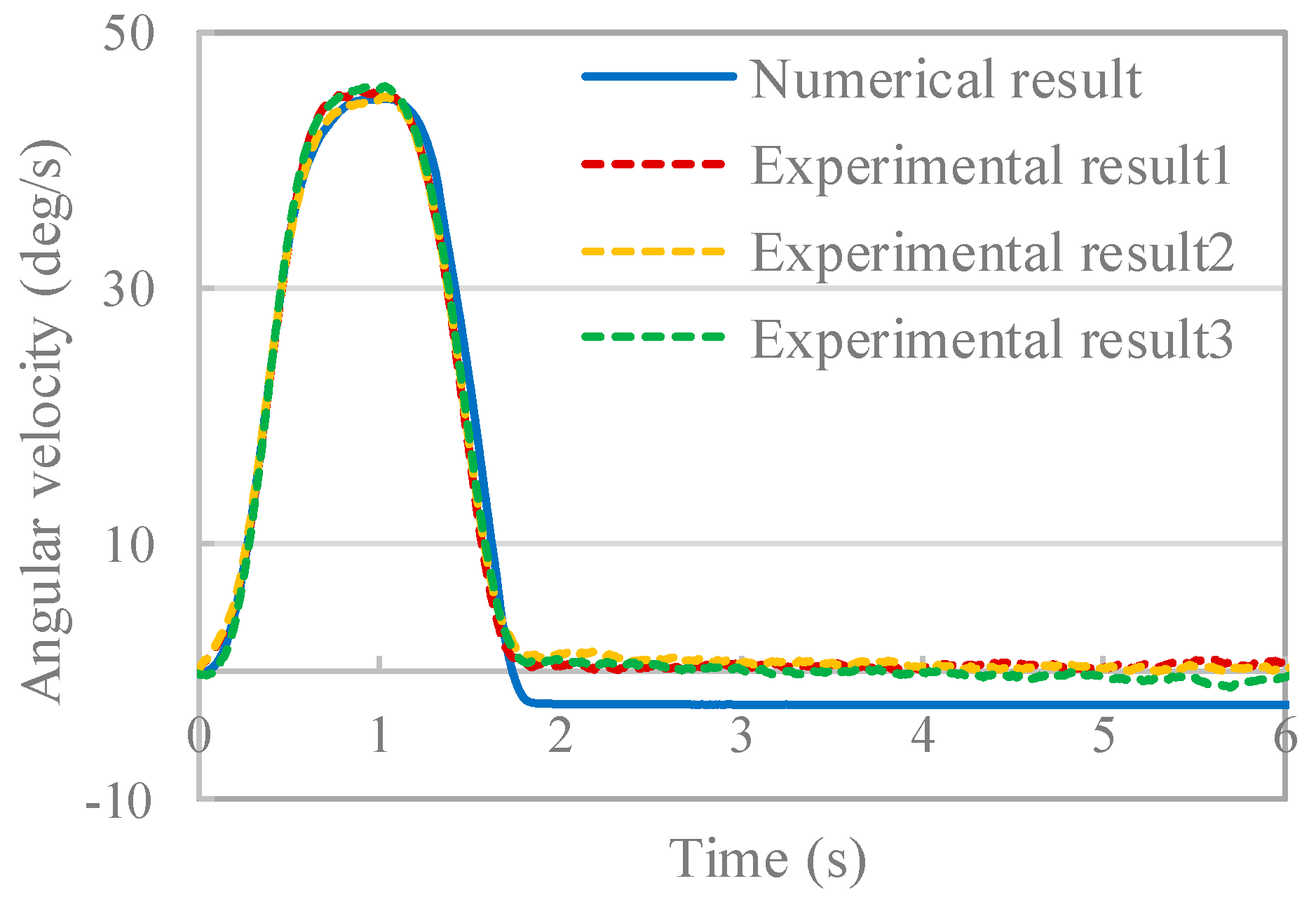
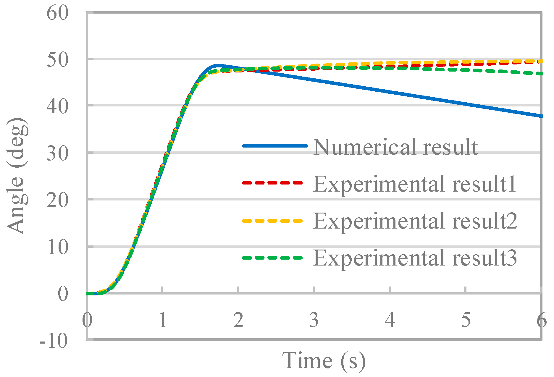
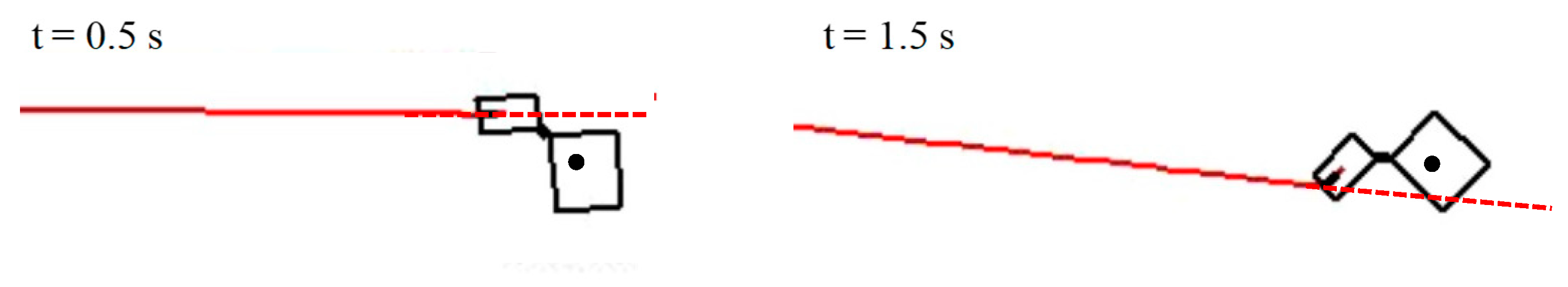
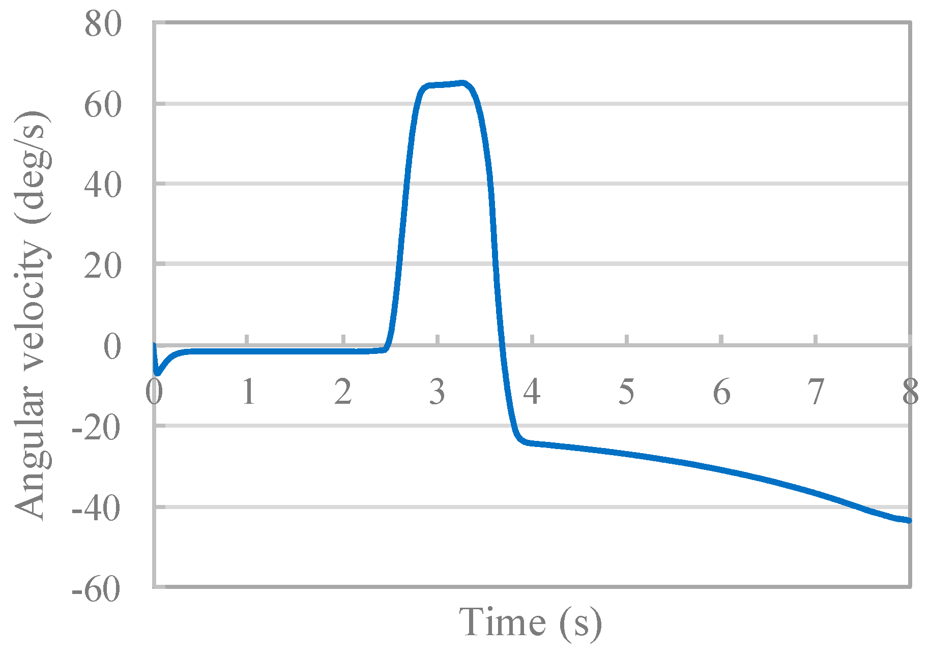
In this section, the numerical simulation and experimental results are compared in order to validate the proposed model. The time history of the angular velocity of the experimental equipment is shown in Figure 9, and the time history of the angle of TSMD is shown in Figure 10. Figure 11 shows the shape of the system at each time during the numerical simulation, and Figure 12 shows the relationship between the COG of the TSMD and the point of action of the tension force at 0.5 s and 1.5 s. From Figure 9 and Figure 10, at 0.0 s to 0.9 s, after winding of the tether is started, the angular velocity and the angle of the experimental equipment suddenly changed. Based on Figure 11, the tether is confirmed to stretch at this time and the TSMD is confirmed to rotate counterclockwise. From 0.9 s to 1.8 s, based on Figure 12, the direct of the tension force changes to apply a clockwise moment to the TSMD, and the angular velocity decreases. As such, the elastic force of the tether and the contact force between the tether and the inlet are considered to greatly influence the movement of the rigid body at 0.0 s to 1.8 s. In other words, the tether motion predominantly determines the motion state of the entire system. After 1.8 s, the angular velocity is confirmed to be constant and the rotational motion continues. Figure 11 indicates that deflection of the tether occurs at this time, and the influence of the tether on the motion of the rigid body becomes small. The inertial motion of the TSMD dominantly determines the motion state of the entire system. Therefore, this system has a feature whereby the motion state of the entire system transits depending on the state of the tether. Next, comparing the results of the numerical analysis with the experiment, the features of the above system are accurately reproduced. A difference of 2.5 deg/s occurred after 1.8 s, but this is considered to be an error caused by, for example, friction in the experimental equipment, because the damping force is not considered in the numerical simulation. In the study of the usefulness of the winding control method, since a large deflection, such as that after 1.8 s, does not occur, the influence of this error is considered to be small. Therefore, the numerical simulation model is reasonable for verifying the usefulness of the proposed control method.

4. Attitude Control When Extending and Winding the Tether

As indicated by the results of the numerical simulation and the experiment, rotational motion occurs in the rigid body system when winding the tether. Therefore, the TSMD requires a mechanism and control in order to suppress the rotational motion that occurs at the time of tether winding and stabilizing the posture. Takehara et al. proposed a control method that changes the direction of the tension acting on the body by the movement of the arm mounted on the TSMD and suppresses the rotational motion of the rigid body generated at the time of winding the tether, and the effectiveness has been confirmed by numerical simulation and experimentally [7]. However, this method requires mounting of a dedicated actuator and has a disadvantage in that the mechanism of the equipment becomes complicated. Therefore, it is desirable that attitude control can be performed using only the tether winding mechanism. Therefore, in the present paper, the attitude control method of the TSMD during tether winding using the change in length of the tether is applied. This method has an advantage in that only one actuator is sufficient. As a control method, control focusing on the sign of the kinetic energy gradient caused by the rotational motion of the system [12] is applied, and the tether winding control method is designed considering the deflection of the tether.

4.1. Winding Control of the Tether Focusing on the Change in Kinetic Energy

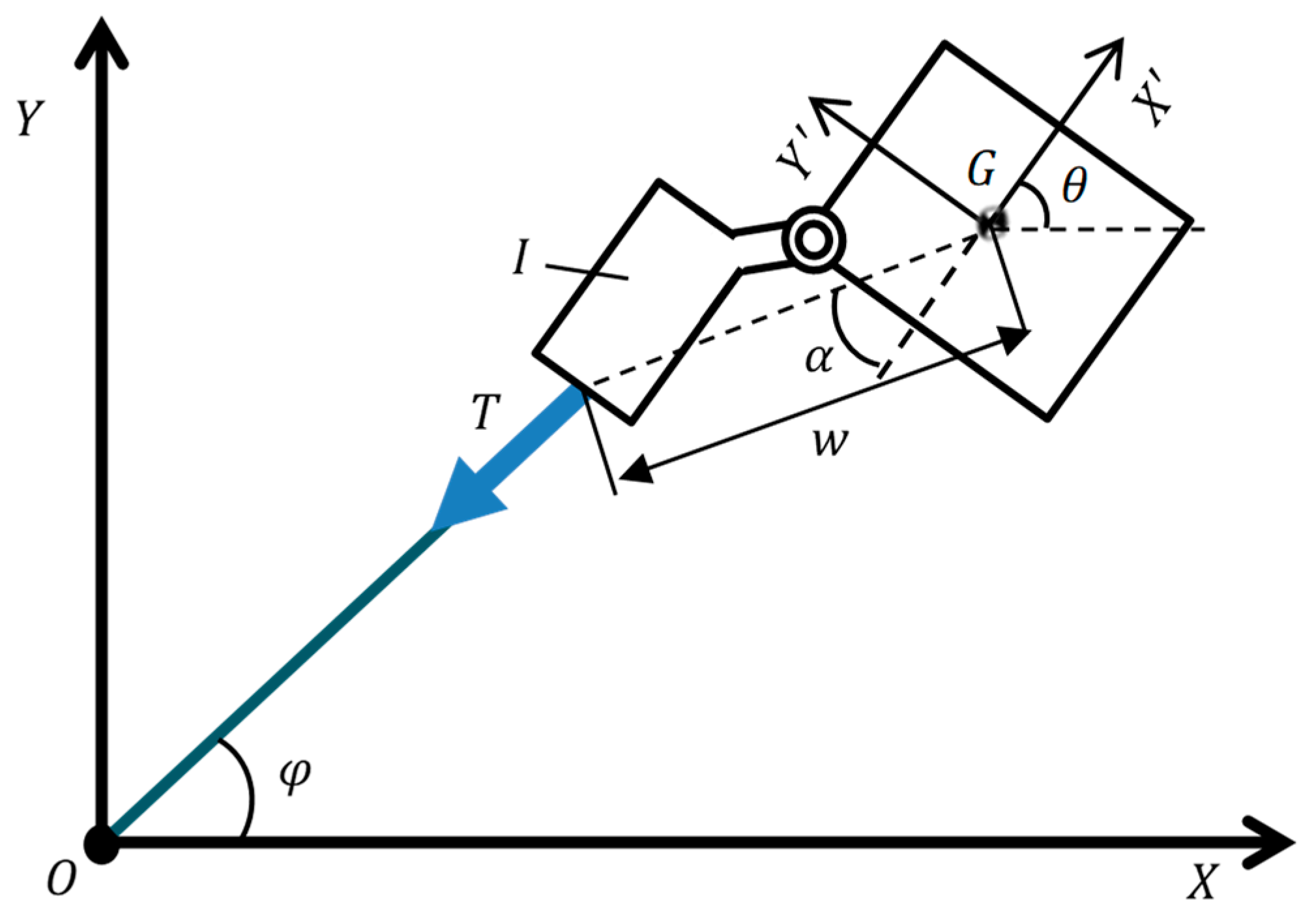
In the tether winding control applied in the present paper, the purpose of control is to converge the angular velocity of the rigid body system generated at tether winding to 0 deg/s. First, a condition in which the tension of the tether damps the rotational motion of the rigid body is derived. Figure 13 shows the model of the TSMD in a state in which the tether is stretched. Here, no relative motion is assumed between the rigid bodies. The symbols in the figure are defined as follows:

• $T$: Tension of the tether
• $\phi$: Angle formed by the tether and the $X$ axis
• $I$: Moment of inertia of the rigid body
• $G$-$X^{\prime }{Y}^{\prime }$: Object coordinate system with the center of gravity $G$ of the rigid body as the origin
• $w$: Distance from $G$ to the tip of the inlet
• $\alpha$: Angle of the tip of the inlet in the object coordinate system
• $\theta$: Rigid body rotation angle

From Figure 13, the equation of motion related to the rotational motion of the rigid body system is given by the following equation:

$$I\ddot{\theta }=wT\sin \left(\phi -\theta +\alpha \right)$$

(44)

The kinetic energy $E_{\theta }$ related to the rotational motion of the rigid body is given by the following equation:

$$E_{\theta }=\frac{1}{2}I{\dot{\theta }}^2$$

(45)

From Equation (45), it turns out that $\dot{\theta }\to 0$ when $E_{\theta }\to 0$. Therefore, by differentiating Equation (45) with respect to time and substituting Equation (44) into the right-hand side of Equation (45), the following equation is obtained:

$${\dot{E}}_{\theta }=I\dot{\theta }\ddot{\theta }=wT\dot{\theta }\sin \left(\phi -\theta +\alpha \right)$$

(46)

Here, from $w>0$ and $T\ge 0$, the following expression holds:

$$\begin{array}{cc}T=0& \dot{\theta }\sin \left(\phi -\theta +\alpha \right)\ge 0\\ T>0& \dot{\theta }\sin \left(\phi -\theta +\alpha \right)<0\end{array}$$

(47)

Switching $T$ as above,

$${\dot{E}}_{\theta }\le 0$$

(48)

$E_{\theta }\to 0$ and $\dot{\theta }\to 0$ with time. Here, $\alpha$ is a system-specific parameter, which is as follows:

$$\alpha \approx 31.57\left[\mathrm{deg}\right]$$

(49)

Next, consider the winding control method of tethers satisfying Equation (47). Let the length of the tether not collected in the rigid body be $l$, and let the target value of the tether length be $r$. Here, for the sake of simplicity, let the transfer function from $r$ to $l$ be:

$$G\left(s\right)=\frac{1}{{\left({\tau }_{l}s+1\right)}^2}$$

(50)

Therefore, $\ddot{l}$ is determined as follows:

$$\ddot{l}=k_{l1}\left(r-l\right)-k_{l2}\dot{l}$$

(51)

And:

$$k_{l1}=\frac{1}{{\tau }_l{}^2}, k_{l2}=\frac{2}{{\tau }_l}, {\tau }_l>0$$

(52)

Moreover, $r$ is determined as follows with reference to Equation (47):

$$\{\begin{array}{cc}r=d+u_{+}& \dot{\theta }sin\left(\phi -\theta +\alpha \right)\ge 0\\ r=d+u_{-}& \dot{\theta }sin\left(\phi -\theta +\alpha \right)<0\end{array}, u_{+}\ge 0, u_{-}\le 0$$

(53)

where $d$ is the distance from the origin of the absolute coordinate system to the tip of the inlet. In addition, $u_{+}$ is the control input when $\dot{\theta }\sin \left(\phi -\theta +\alpha \right)\ge 0$, and $u_{-}$ is the control input when $\dot{\theta }\sin \left(\phi -\theta +\alpha \right)<0$. These values are constants in the present paper. By defining $r$ as Equation (53), the tether deflects when the tension is working to increase the kinetic energy of the rigid body, and the tether stretches when the tension works to reduce the kinetic energy of the rigid body. By repeating this cycle, it is possible to converge the angular velocity of the rigid body system to 0 deg/s over time.

4.2. Prevention of Chattering by Hysteresis

Figure 14 shows the control input in the winding control shown in the previous section. As shown in Figure 14a, in the control rule given by Equation (53), the control input is switched by the sign of $\dot{\theta }\sin \left(\phi -\theta +\alpha \right)$. Therefore, when the angular velocity converges to around 0 deg/s by control, it is considered that a phenomenon called chattering occurs in which the control input violently switches. Since the occurrence of chattering may cause a malfunction of the electronic device, in order to prevent this, hysteresis is set for switching the control input. As shown in Figure 14b, the threshold value for switching the control input is given as a width, and once the control input becomes $u_{-}$, the value of $\dot{\theta }\sin \left(\phi -\theta +\alpha \right)$ reaches the set value a, and design switching is not performed until the control input is exceeded. Here, we set a as:

$$\{\begin{array}{cc}a=a_1& {\dot{\theta }}_3>{\omega }_c\\ a=a_2& {\dot{\theta }}_3\le {\omega }_c\end{array}\hspace{1em}(a_2>a_1)$$

(54)

where ${\dot{\theta }}_3$ is the angular velocity of the human analog, and ${\omega }_c$ is the threshold value (constant) of the angular velocity. When the angular velocity of the rigid body system is large, the hysteresis width is set to be small in order to improve the control accuracy. The hysteresis width is set to be large when the rigid body posture is sufficiently stable, and the angular velocity falls below the threshold value ${\omega }_c$, so that the control input does not easily change. By following the above procedure, the occurrence of chattering can be prevented while maintaining the accuracy of the attitude control effect by performing control while changing the value of a.

4.3. Numerical Simulation Conditions

The effectiveness of the proposed control is verified using a numerical simulation model that considers the shooting and extension of the tether. The numerical simulation conditions are shown in

Table 2. Condition of numerical simulations.

Condition	${\mathit{\tau }}_{\mathit{l}}$	${\mathit{u}}_{+}$	${\mathit{u}}_{-}$	Setting Value
Without control	-	-	-	-
Control 1	0.1	0.02	−0.03	$\begin{array}{c}{a}_1={1.5310}^{-6}\\ a_2={1.0310}^{-3}\\ {\omega }_c=0.001\end{array}$
Control 2	0.1	0.02	−0.03	a = 1.5 × 10−6
Control 3	0.1	0.02	−0.03	-

. Without control is a condition for constant-speed winding. Control 1 is a condition that considers hysteresis in which winding control is applied, and a is variable. Control 2 is a condition in which a is a constant value, and control 3 is a condition in which hysteresis is not considered. The values of $u_{+}, u_{-}$, and ${\tau }_l$ are unchanged for all conditions. Moreover, for all conditions, winding starts at the moment the tip of the tether is attracted to the target point.

Table 3. Calculation parameters.

Distance to the attachment position (m)	2.0
Mass of the tip of the tether (kg)	0.1
Distance from natural length to the point mass (m)	0.3
Spring constant for shooting the tip k (N/m)	100
Spring constant for attaching the tip $k_a$ (N/m)	1000
Target deflection during tether extension $l_{et}$ (m)	0.01
Gain of drive constraint during tether extension $K_e$	10

shows the initial conditions and calculation parameters of numerical simulation for all conditions. Parameters that are not shown in Table 3 are the same as in Section 3. The analysis time was set to 8.0 s for the condition without control and to 14.0 s for the conditions in which controls 1 through 3 are applied.

4.4. Numerical Simulation Results and Discussion

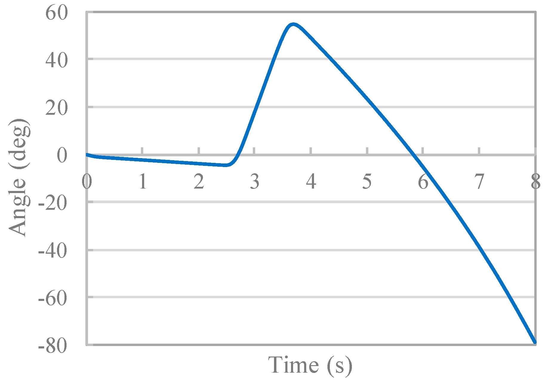
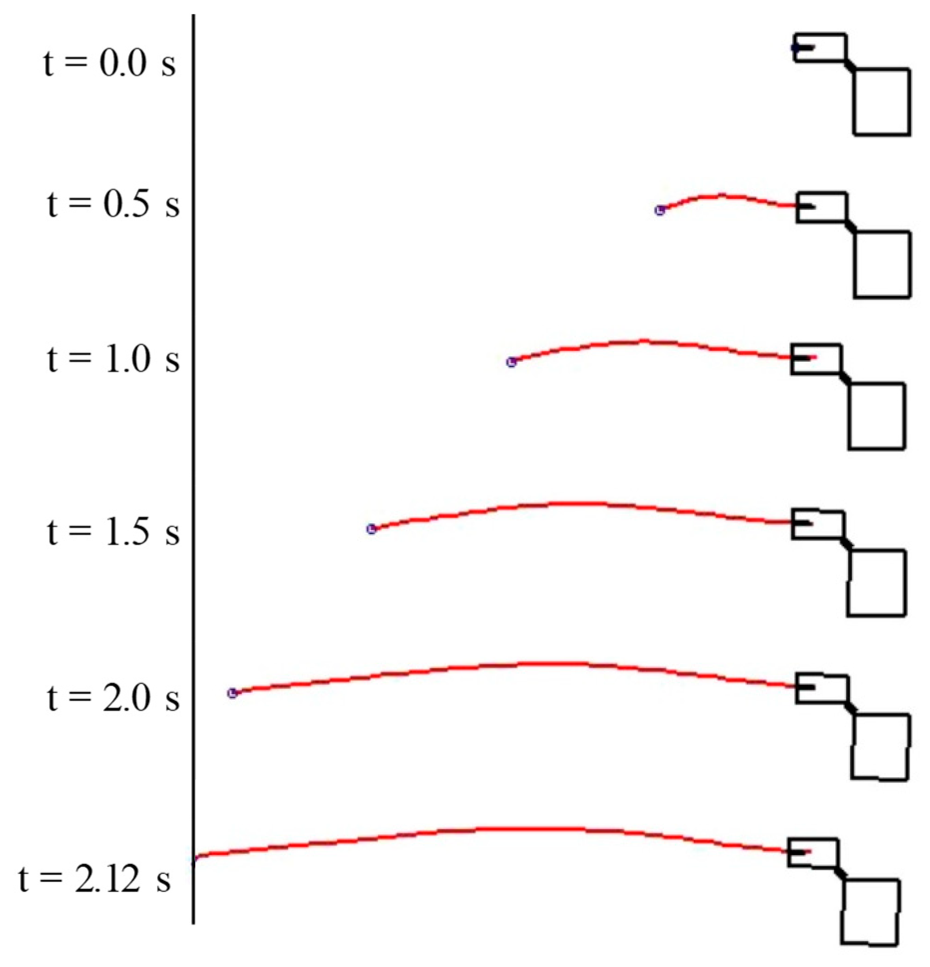
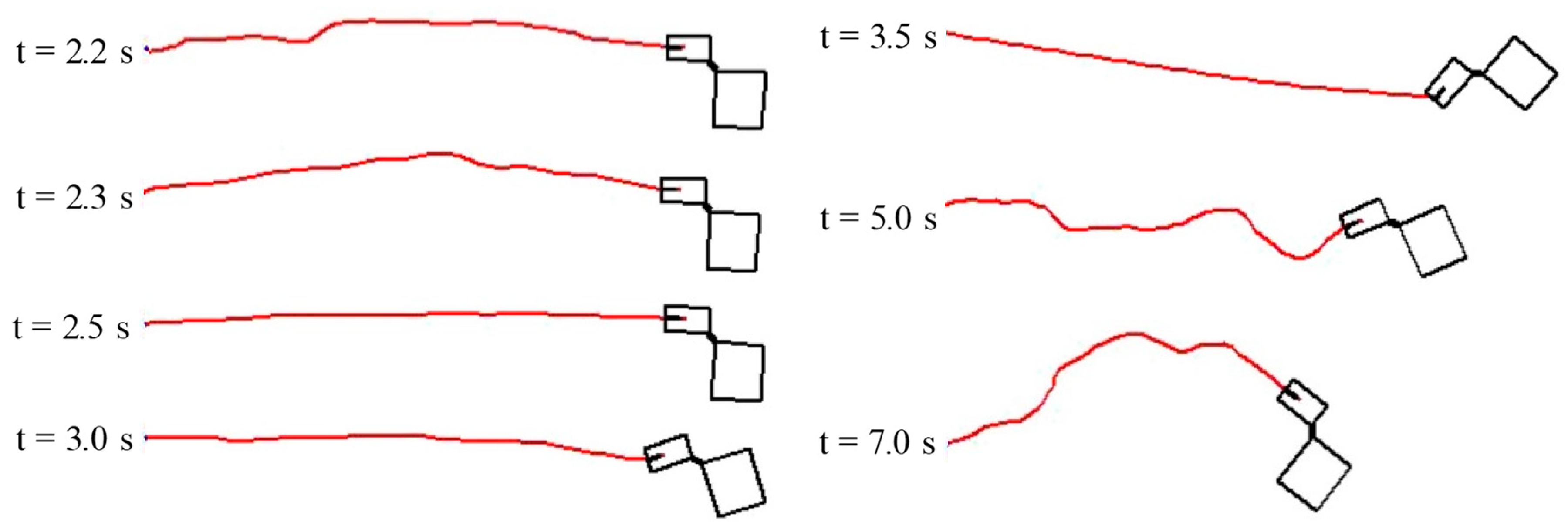
Figure 15 and Figure 16 show the time history of angular velocity and angle under the condition without control. Even in the analysis considering the tether extension, as well as the analysis result shown in Section 3, a large deflection of the tether occurred, and the rotational motion of the rigid body was confirmed to continue. Differences in rigid body movement caused by the presence or absence of tether extension are described below. At 0.0 s, extension of the tether is started by shooting the tether tip. At 2.12 s, the tether tip attaches to the destination, and winding of the tether is started at the same time. Figure 17 shows the shape of the system during tether extension. Shooting the tether is performed by adding a spring force applied to the tip of the tether from 0.0 s. At this time, a reaction force due to shooting is also applied to the rigid body side, and a rotational motion of 1.5 deg/s is generated clockwise in the rigid body. As shown in Figure 17, the shape of the tether is bent in the positive direction of the Y axis during extension. The cause of this phenomenon is the contact force in the positive direction of the Y axis generated by the tether being in contact with the lower suction port due to the clockwise rotation of the rigid body system. Then, the tip of the tether is attached at the destination at 2.12 s, and winding of the tether is started immediately thereafter. Figure 18 shows the shape of the system during tether winding. The impact force generated when the tether is attached is propagated through the tether at 2.2 s and 2.3 s. All of the deflections that occurred during tether extension are wound up at 2.5 s, and the angular velocity and angle of the rigid body change greatly due to stretching of the tether. The maximum value of the angular velocity is larger than that in Figure 9, which is considered to be due to the large tension acting on the tether because the rigid body was rotating at an angular velocity of −1.5 deg/s. Thereafter, as shown by t = 3.0 s in Figure 18, the angular velocity is constant from 2.8 s to 3.3 s due to the deflection of the tether. The tether was stretched as a result of the rotation of the rigid body at 3.3 s, a large tension was again generated, and the angular velocity sharply decreased. The rigid body then continued its clockwise rotation movement.

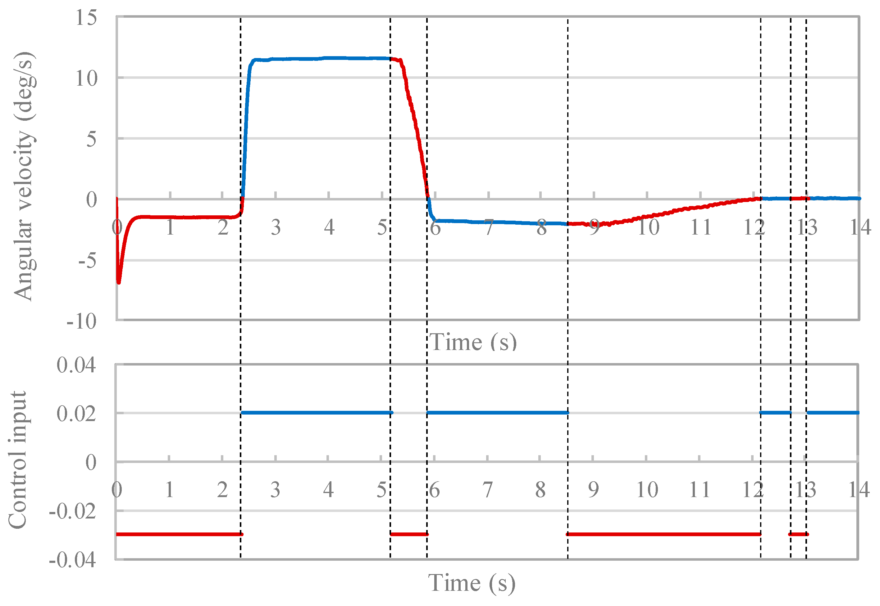
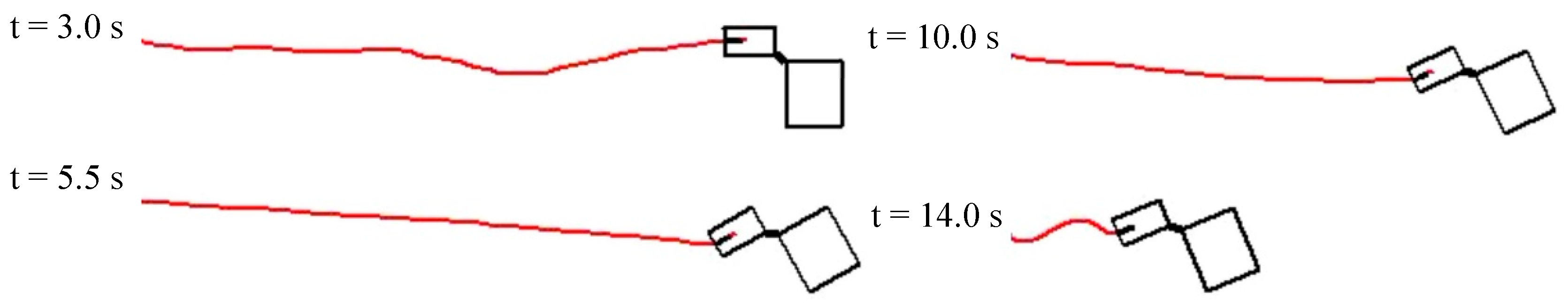
Figure 19 shows the time history of the angular velocity and the time history of the control input in control 1, and Figure 20 shows the shape of the system during tether winding in control 1. Similar to the condition without control, the tether is extended from 0.0 s, and winding of the tether is started at 2.12 s. Immediately after the start of tether winding, the control input becomes $u_{+}$ ($u$ = 0.02), so that the tether is deflected, and the angular velocity in the rigid body system is suppressed. Under the condition without control, the angular velocity increased to 65 deg/s, whereas with control 1, the maximum value of the angular velocity is 11.5 deg/s. Thereafter, from 5.2 s to 5.9 s, the control input is switched to $u_{-}$ ($u$ = −0.03), the tether is stretched, and the tension acts in a direction that decreases the kinetic energy, whereby the angular velocity decreases. From 5.9 s to 8.5 s, the control input again becomes $u_{+}$ in order to prevent the kinetic energy of the rigid body from increasing by tether bowing. Even after 8.5 s, the control input is switched three times, and the angular velocity of the rigid body system converges to 0 deg/s with time. Based on the considerations, the tether deflects when the tension is working to increase the kinetic energy of the rigid body system, and the tether stretches when the tension works to reduce the kinetic energy of the rigid body, which indicates that the proposed winding control is effective for attitude control.

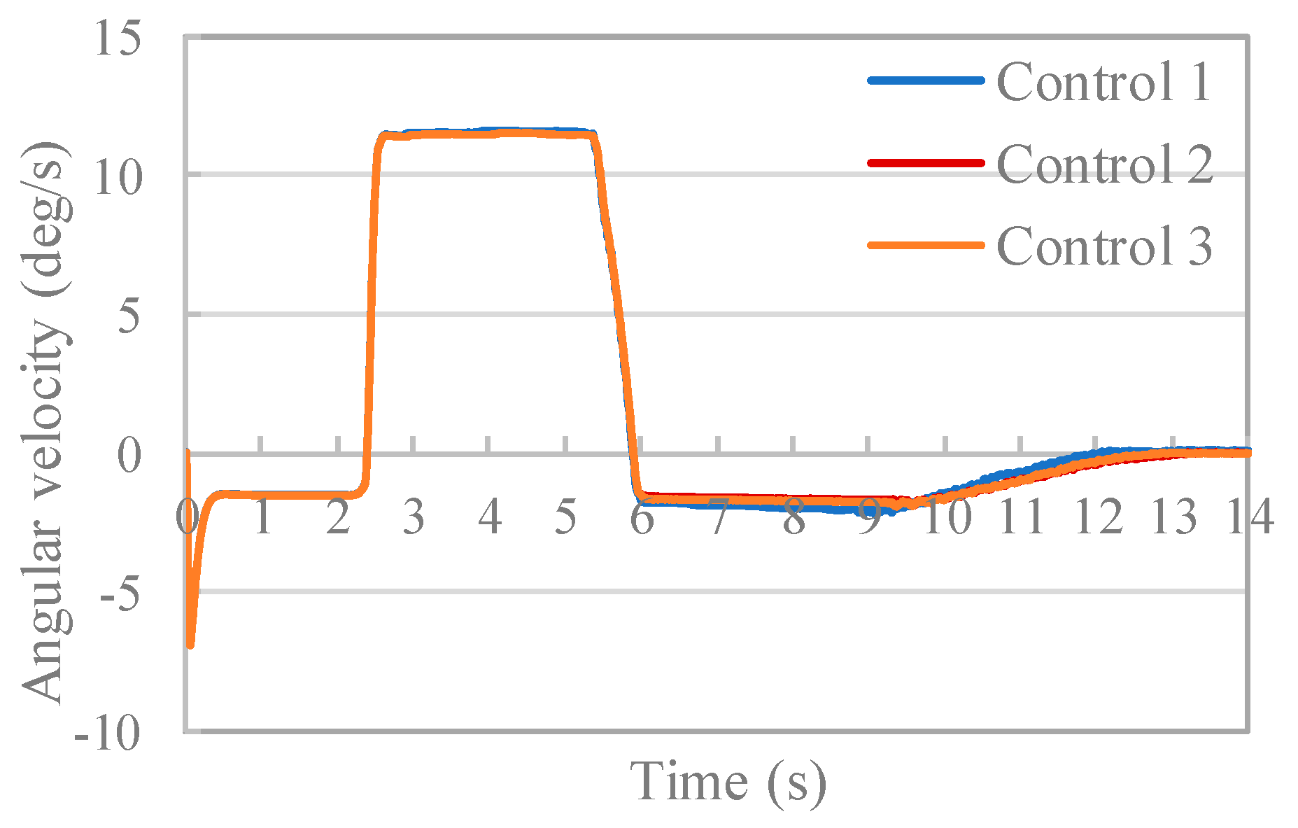
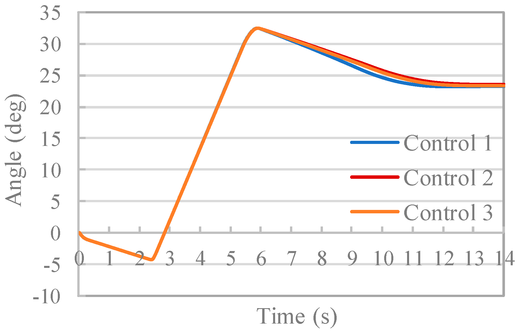
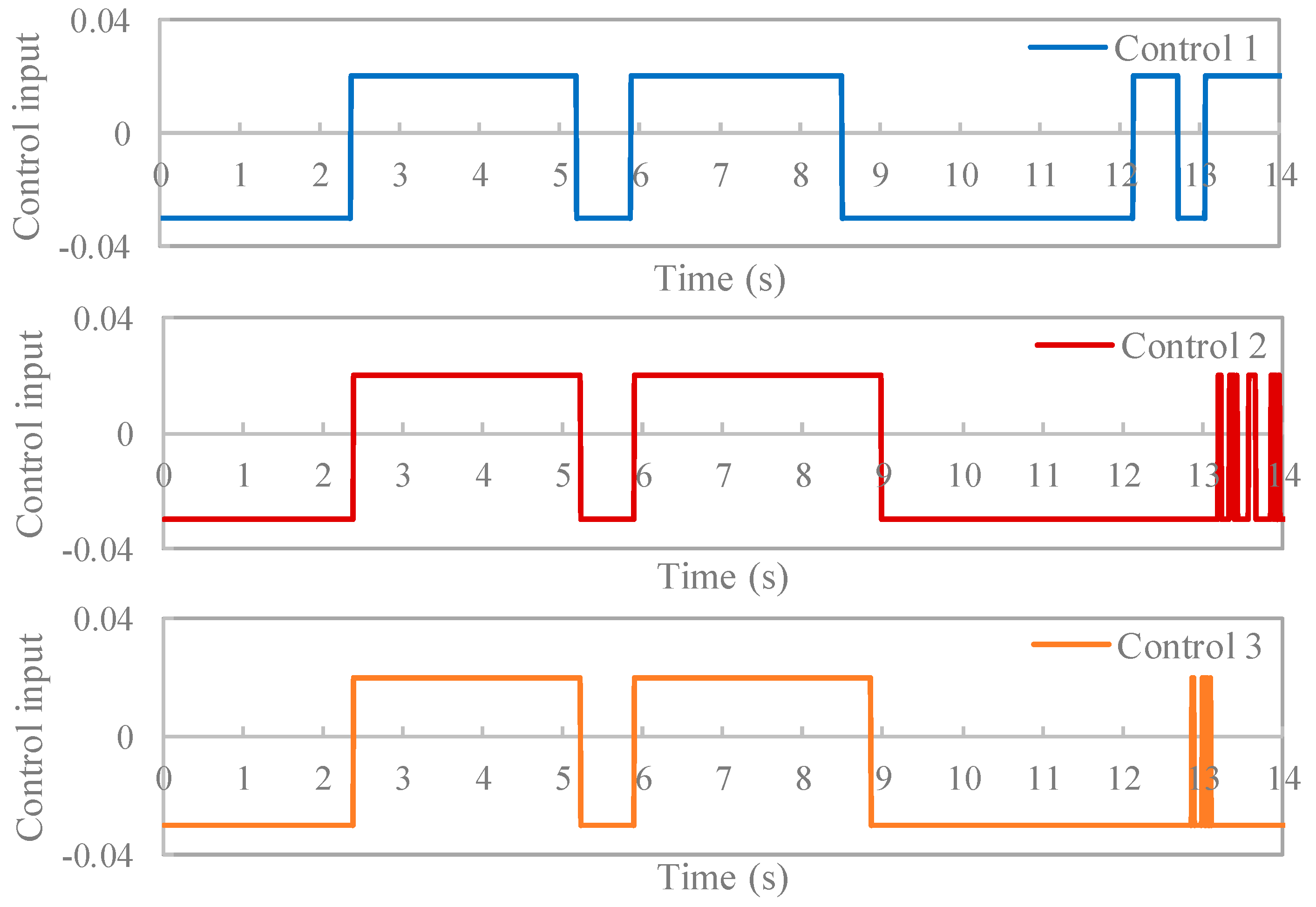
Next, the effect of preventing control input chatter by hysteresis setting will be described. Figure 21 and Figure 22 show the time history of the angular velocity and the time history of angles, respectively, for controls 1 through 3, and Figure 23 shows the time history of the control input under each condition. Figure 23 indicates that, for controls 2 and 3, chattering occurs after 13 s when the attitude of the rigid body is stable. On the other hand, in control 1, control can be performed without causing chattering. Furthermore, from Figure 21, the angular velocity is confirmed to converge to 0 deg/s under each condition, and an effective attitude control effect is obtained. At this time, the average value of the angular velocity after 13 s and achieving a stable attitude is −0.054 deg/s for control 1, −0.012 deg/s for control 2, and −0.020 deg/s for control 3. In control 1, the convergence value is somewhat larger than the other conditions, but converged to a sufficiently small value, and the attitude control was performed with high accuracy. Based on the above results, highly accurate attitude control was obtained without causing chattering in the control input by applying a winding control method with the hysteresis setting value changing according to the rigid body angular velocity proposed in Section 4.1.

5. Conclusions

In the present paper, as a fundamental study of a TSMD system intended for use in microgravity environments, we constructed an analytical model based on multibody dynamics and analyzed the TSMD motions during tether extension and winding operations. The validity of the analytical model was confirmed by an experiment reproducing 2D microgravity. We also proposed a winding control method that uses the amount of tether deflection and the kinetic energy gradient of the experimental equipment using the proposed model. By applying the control, the rotational motion of the rigid body system was suppressed, and the angular velocity was confirmed to converge to 0 deg/s. Based on this result, effective attitude control was demonstrated by the proposed winding control. Furthermore, by setting the hysteresis in switching control, highly accurate attitude control was confirmed to be obtained while preventing the occurrence of chattering in the control input. Some important developments are planned for the future. First, cases when some disturbances occur should be considered. From the numerical results, it is found that when the position of the center of gravity of the system changes due to disturbance, the accuracy of the attitude control decreases. This is because the parameters related to the position of the center of gravity of the system are included in the control method. Therefore, to adopt the proposed control method in an actual system, an estimation method of the position of the center of gravity of the system must be taken into account. Second, measurement of the tether length makes instruments complicated; therefore, estimation of the tether length using only sensor information of the TSMD will be considered.

References

- Chen, Y.; Huang, R.; He, L.; Ren, X.; Zheng, B. Dynamical modelling and control of space tethers: A review of space tether research. Nonlinear Dyn. 2014, 77, 1077–1099. [Google Scholar] [CrossRef]
- Nohmi, M. Space verification experimental analysis for attitude control of a tethered space robot. Trans. JSME 2014, 80. [Google Scholar] [CrossRef]
- Watanabe, T.; Fujii, H.; Kojima, H.; Singhose, W. Design of electric current profile for electrodynamic tether systems by input shaping method. J. Jpn. Soc. Aeronaut. Space Sci. 2005, 53, 569–576. [Google Scholar]
- Aslanov, S.V.; Ledkov, S.A. Dynamics of towed large debris taking into account atmospheric disturbance. Acta Mech. 2014, 225, 2685–2697. [Google Scholar] [CrossRef]
- Sabatini, M.; Gasbarri, P.; Palmerini, B.G. Elastic issues and vibration reduction in a tethered deorbiting mission. Adv. Space Res. 2016, 57, 1951–1964. [Google Scholar] [CrossRef]
- Huang, P.; Hu, Z.; Zhang, F. Dynamic modelling and coordinated controller designing for the maneuverable tether-net space robot system. Multibody Syst. Dyn. 2016, 36, 115–141. [Google Scholar] [CrossRef]
- Takehara, S.; Nishizawa, T.; Kawarada, M.; Hase, H.; Terumichi, H. Development of tether space mobility device. Comput. Methods Appl. Sci. 2014, 35, 255–274. [Google Scholar]
- Shabana, A.A. Dynamics of Multibody Systems, 3rd ed.; Cambridge University Press: Cambridge, UK, 2005. [Google Scholar]
- Berzeri, M.; Shabana, A.A. Development of simple models for the elastic forces in the absolute nodal co-ordinate formulation. J. Sound Vib. 2000, 235, 539–565. [Google Scholar] [CrossRef]
- Wago, T.; Kobayashi, K.; Sugawara, Y. Improvement on evaluating axial elastic force in beam element based on the absolute nodal coordinate formulation by accurate mean axial strain measure. Trans. Jpn. Soc. Mech. Eng. 2013, 79, 2704–2713. (In Japanese) [Google Scholar] [CrossRef]
- Komatsu, T.; Uenohara, M.; Iikura, S.; Murata, H.; Shimoyama, I. The development of an autonomous space robot operation testbed. J. Robot. Soc. Jpn. 1990, 8, 712–720. [Google Scholar] [CrossRef]
- Murakami, W.; Shimachi, S.; Hagihara, Y.; Hashimoto, A.; Hakozaki, Y. Cargo transfer by tethered satellite system. Trans. JSME 2006, 41, 169–170. (In Japanese) [Google Scholar]
Figure 1.
Tether Space Mobility Device (TSMD) concept.
Figure 2.
Analytical model outline.
Figure 3.
Beam element.
Figure 4.
Flexible body element drawn into rigid body 1.
Figure 5.
Flexible body element drawn into rigid body 1 (enlarged view).
Figure 6.
Outline of the analytical model of attaching the tether tip.
Figure 7.
Experimental equipment of the TSMD.
Figure 8.
Initial experiment and analysis conditions.
Figure 9.
Time history of angular velocity.
Figure 10.
Time history of angle.
Figure 11.
Shape of the system by numerical simulation.
Figure 12.
Relationship between the center of gravity (COG) of the TSMD and the point of action of the tension force at 0.5 s and 1.5 s.
Figure 13.
Model of the TSMD when the tether is under strain.
Figure 14.
Time history of the control input.
Figure 15.
Time history of angular velocity (without control).
Figure 16.
Time history of angle (without control).
Figure 17.
Shape of the system during tether extension (without control).
Figure 18.
Shape of the system during tether winding (without control).
Figure 19.
Time history of angular velocity and control input (control 1).
Figure 20.
Shape of the system during tether winding (control 1).
Figure 21.
Figure 22.
Figure 23.
Time history of the control input (controls 1 through 3).