Reduced Order Controller Design for Symmetric, Non-Symmetric and Unstable Systems Using Extended Cross-Gramian

1
Department of Electrical Engineering, College of Electrical and Mechanical Engineering, National University of Sciences and Technology (NUST), Islamabad 44000, Pakistan
2
School of Electrical, Electronic and Computer Engineering, The University of Western Australia, Perth 6009, Australia
*
Author to whom correspondence should be addressed.
Machines 2019, 7(3), 48; https://doi.org/10.3390/machines7030048
Submission received: 28 February 2019
/
Revised: 8 May 2019
/
Accepted: 10 May 2019
/
Published: 29 June 2019
(This article belongs to the Special Issue Selected Papers from Conference on Control, Mechatronics and Automation (ICCMA))
Abstract
:In model order reduction and system theory, the cross-gramian is widely applicable. The cross-gramian based model order reduction techniques have the advantage over conventional balanced truncation that it is computationally less complex, while providing a unique relationship with the Hankel singular values of the original system at the same time. This basic property of cross-gramian holds true for all symmetric systems. However, for non-square and non-symmetric dynamical systems, the standard cross-gramian does not satisfy this property. Hence, alternate approaches need to be developed for its evaluation. In this paper, a generalized frequency-weighted cross-gramian-based controller reduction algorithm is presented, which is applicable to both symmetric and non-symmetric systems. The proposed algorithm is also applicable to unstable systems even if they have poles of opposite polarities and equal magnitudes. The proposed technique produces an accurate approximation of the reduced order model in the desired frequency region with a reduced computational effort. A lower order controller can be designed using the proposed technique, which ensures closed-loop stability and performance with the original full order plant. Numerical examples provide evidence of the efficacy of the proposed technique.
1. Introduction
The practical systems that occur in nature are mostly represented by higher order mathematical models. The analysis required for these large-scale systems to design and implement a controller is cumbersome because the controller design methods yield controllers of order at least equal to the original system, if not greater. Model order reduction (MOR) techniques simplify this problem by constructing a reduced order model (ROM), which enables a reduced order controller design for higher order plants that is practically feasible for implementation [1].
Moore [2] presented a MOR technique based on an internally balanced state-space realization of the full order model (FOM). The controllability and observability gramians of a balanced state-space realization are equal and diagonal. Each state in a balanced realization is equally controllable and observable. The ROM in balanced truncation is then obtained by discarding the weakly controllable and observable states. Balanced realization only exists if the original FOM is stable and minimal. For non-minimal systems or even systems with nearly uncontrollable or unobservable states, the computation of balanced realization suffers ill-conditioning [3,4]. Resultantly, the approximation error in balanced truncation is increased if the system is close to non-minimality. This numerical difficulty in balanced truncation can be avoided by using a balancing free algorithm [4] based on Schur-decomposition, which does not require the original system to be minimal and constructs an approximate balanced-realization of FOM.
The cross-gramian has been the focus of many researchers in MOR and system theory for large-scale systems where computational complexity and simulation time is a challenge. Since its inception by Fernando and Nicholsen [5], for stable single-input-single-output (SISO) systems, many questions arose for its applicability towards practical systems, which may be multi-input-multi-output (MIMO) (symmetric and non-symmetric), and/or even unstable systems. This has opened new avenues for the calculation of a more general cross-gramian. Laub, Silverman, and Verma [6] and Fernando [7] extended the cross-gramian for symmetric MIMO systems. The cross-gramian introduced in [6,7] can only be computed for symmetric systems. The property that makes cross-gramian useful in MOR is that it contains conjoined information of both controllability and observability gramian. Thus, two Lyapunov Equations that define the controllability and observability gramians can be replaced with a single Sylvester Equation and thus the computational cost can significantly be reduced [8]. There also exists some methods in the literature that expand the scope of cross-gramian to non-symmetric systems such as [9,10,11,12]. Aldhaheri in Reference [13] presented a cross-gramian-based algorithm for finding Moore’s balanced realization [2] ROM, which does not require the original system to be minimal. However, this algorithm is restricted to SISO and symmetric MIMO systems.
Generally, two approaches are used to design a lower order controller for a full order plant: Plant reduction and compensator reduction [14]. In plant reduction, an ROM of the original full order plant is obtained using MOR techniques such that if a lower order controller is designed for the reduced plant, it satisfies the closed-loop performance criteria with the full order plant. In compensator reduction, first, a higher order controller is designed for the full order plant and then MOR is applied to obtain a reduced order controller which satisfies the closed-loop performance criteria with the original plant. The compensator reduction approach is more accurate than the plant reduction approach, and hence it is preferred [15]. Plant reduction requires some knowledge of the controller to be designed in advance for its implementation. Since the approximation is done before the controller design, its accuracy is inferior to compensator reduction, wherein both the plant and controller are known before the reduction. However, in situations where it is difficult or impossible to design a controller for a high order plant beforehand, plant reduction is a good design tool. Despite the importance of plant reduction, it has been mostly ignored in the control system literature. In power system literature, it is customary to reduce the plant before designing a damping controller to mitigate inter-area oscillations, however, most of the researchers completely ignore the closed-loop performance in the reduction process; see References [16,17,18] for an instance. This is against the motivation of both the plant and compensator reduction as a lower order controller cannot be obtained by simply picking any MOR technique and applying it to the plant/controller. A MOR technique that incorporates the closed-loop performance in its reduction criteria is feasible for the plant/compensator reduction.
Various closed-loop performance criteria can be written as frequency-weighted approximation criteria. Enns in [19] generalized Moore’s balanced truncation [2] and presented frequency-weighted balanced truncation (FWBT) by introducing frequency weights which ensures the accuracy of ROM over the frequency range emphasized by the frequency weights. FWBT can thus be used for both plant and compensator reduction problems. Later, Zulfiqar proposed a frequency-weighted cross-gramian based FWBT algorithm for SISO system in Reference [8]. This algorithm is applicable to non-minimal systems as well. A common issue in plant/compensator reduction is that frequency weights, which define the closed-loop performance criteria, become unstable if the plant has transmission zeros in the right half of the s-plane. Both the algorithms of FWBT in References [19] and [8] only work if both the plant and the frequency weights are stable. This limits their applicability to many plant/compensator reduction problems.
As mentioned earlier, plant reduction did not get its due coverage in the literature despite being an important problem. Recently, a cross-gramian -based plant reduction algorithm is presented in Reference [20], which is less computational than Enns’ plant reduction algorithm (EPRA) [19]. The algorithm has also shown quicker convergence than Reference [19] and it is less prone to ill-conditioning due to the use of cross-gramian for the reasons discussed earlier in this section. This algorithm, however, is only applicable to stable SISO systems. In this paper, we generalize this algorithm to extend its applicability to a wide range of systems. We propose a unifying framework that extends the applicability of the algorithm in Reference [20] to the stable, unstable, symmetric, and non-symmetric MIMO systems. The unifying framework is based on the developments made in the literature to extend the definition of cross-gramian for non-symmetric MIMO systems and unstable systems. We generalize the definition of frequency-weighted cross-gramian given in Reference [8] to include the aforementioned classes of systems.
The paper is organized as follows. Section 2 provides the necessary background and survey of the cross-gramian, frequency-weighted model reduction, and controller reduction problem. Section 3 presents the main results of the paper. Section 4 shows the experimental results and comparisons. Section 5 discusses the results obtained, whereas Section 6 concludes the paper.
2. Preliminaries
Consider a continuous time full order stable system
The transfer function (TF) can be represented as
where , , , .
2.1. Cross-Gramian for Symmetric Systems
It is assumed that the system is square and symmetric i.e., , and the number of inputs is equal to the number of the outputs . The controllability , observability and cross gramians [5] are defined as
which satisfy the following respective Lyapunov and Sylvester Equations:
For SISO and symmetric MIMO systems, the cross-gramian possess a unique relation [5] with Hankel singular values of the original system
where . This property holds true for all SISO systems because all SISO systems are symmetric. However, for non-symmetric MIMO systems, the above property does not hold in general.
2.2. Cross-Gramian for Non-Symmetric Systems
The non-symmetric MIMO systems are an important category of control systems. Many physical dynamical systems are non-symmetric in nature. The problem with such systems is that they do not preserve the basic property of cross-gramian defined in Equation (3). In the literature, many extensions exist to broaden the scope of cross-gramian for non-symmetric systems [9,10,11,12]. There is some abuse in the usage of mathematical variables in the following subsections. However, the context clearly shows the difference.
2.2.1. Symmetrizer Based Approach
The symmetrizer -based approach [10,11,21] finds an approximate cross-gramian for non-symmetric systems. The idea is based on finding a symmetrizer [21] to embed a non-square or non-symmetric square system into a symmetric system [10,11]. The relation between and the state system matrix is given by . The augmented system obtained from embedding is given by
![Machines 07 00048 i001]()

The approximate cross-gramian is then defined as
which satisfies the following Sylvester Equation
This approximate cross-gramian does not satisfy the basic property (3) but approximates it.
2.2.2. Average Cross-Gramian Using System Decomposition
A non-symmetric MIMO system can be partitioned into SISO systems based on the concepts of decentralized control to compute an average cross-gramian for these systems [12]. Let the state-space matrices of a MIMO system with -inputs and -outputs be decomposed as
and
Definition 1.
The average cross-gramian is the sum of all
SISO subsystem’s cross gramians.
satisfies the following Sylvester Equation
2.3. Enns’ FWBT
In this subsection, Enns’ FWBT [19] technique is discussed. Define the input and output weights as
respectively. The objective of frequency-weighted MOR (FWMOR) problem is to find a ROM
of order such that (9) is small.
Let the augmented system and be represented as
where
The controllability and observability gramians of the augmented systems are defined as
which satisfy the following Lyapunov Equations:
The blocks of Equations (11) and (12) corresponding to can be written as
The transformation matrix is computed as where and . Here are the frequency-weighted Hankel singular values. The transformed state-space realization becomes
where is the ROM of .
2.4. Cross-Gramian Based FWMOR
In [20], a frequency-weighted cross-gramian based MOR algorithm is presented for SISO systems which requires only the solution of one Sylvester Equation instead of two Lyapunov Equations. The algorithm is less computational than Enns’ FWBT and the ROM is as accurate as obtained from FWBT. Let the augmented system be represented with the following state-space realization
![Machines 07 00048 i002]()

The cross-gramian of the augmented system satisfies the following Sylvester Equation
can be partitioned according to the state-space realization in Equation (17) as
The frequency-weighted cross-gramian solves the following Sylvester Equation
The similarity transformation in frequency-weighted cross-gramian based FWMOR is computed as where are the eigenvalues of the , which are directly related to the frequency-weighted Hankel singular values. The original system is thus transformed using the similarity transformation and then truncated to obtain an ROM, as in FWBT.
3. Main Work
In this section, we present a plant reduction algorithm based on the frequency-weighted cross-gramian. A brief version of this algorithm appeared in [20] wherein it was only applicable to SISO systems that are stable. In this paper, we present a unifying framework to extend the applicability of the algorithm to unstable and/or non-symmetric systems. The proposed plant reduction algorithm is also an iterative algorithm like EPRA [19], but it converges faster than EPRA. The proposed algorithm is less computational as it uses cross-gramian based FWMOR instead of FWBT. It is also computationally more stable as cross-gramian based FWMOR is less prone to ill-conditioning particularly when the system is non-minimal or nearly non-minimal. Moreover, the proposed algorithm can also handle unstable plants. Since the compensator reduction is more accurate than the plant reduction, we propose to reduce the order of plant in the plant reduction only to an extent that the controller design package can easily handle this reduced plant. The controller obtained may still be of a high order, but this can be further reduced with much accurate compensator reduction. It is evident from the simulation results in Section 4 that the controller obtained with this hybrid approach yields a better loop shape despite being compact.
Consider a stable realization of the full order plant of order
where . The objective is to find a controller of order such that some closed-loop performance criterion with is achieved. Let be an order ROM of the full order plant such that is low enough for the controller design package to handle. Let be a stabilizing controller designed for and the closed-loop TF with and is given by
According to the stability robustness theorem [14], is also a stabilizing controller for if either or is satisfied, i.e.,
or
It is evident from and that plant reduction is a FWMOR problem, i.e.,
with the following frequency weights
respectively. Since and depend both on and which are not known a priori, some mathematical manipulation is required to incorporate them in the approximation criteria of MOR procedure. The loop shaping controller design procedures help in removing the dependence on because the loop TF or is known a priori, i.e., or . Consider first, and can be done similarly by analogy. Let the desired closed-loop TF for the loop shaping be . can be represented independently of as .
The weight still depends on which is not known a priori, and thus the plant reduction problem under consideration becomes an iterative problem. is initialized with initially and the reduced plant is obtained using cross-gramian based FWMOR. If has transmission zeros in the right half of the s-plane, becomes unstable, and the frequency-weighted cross-gramian cannot be computed for even if is a SISO system. Similarly, if is unstable, the frequency-weighted cross-gramian cannot be computed for even if is a SISO system. Inspired by References [22] and [23], we generalize the computation of frequency-weighted gramians for unstable systems. Let the state-space realizations of and be
![Machines 07 00048 i003]()

If is stabilizable, a symmetric matrix exists which solve the following Riccati Equation
can be partitioned according to , i.e.,
Define and as
when and are Hurwitz, is Hurwitz and . However, when and/or are not Hurwitz, is not Hurwitz, but is Hurwitz. Now there can be two cases, i.e., either is a symmetric or a non-symmetric system. If is a symmetric system, the frequency-weighted cross-gramian for the realization of can be computed by solving the following Sylvester Equation
where is the block of (25) corresponding to .
If is a non-symmetric system, the frequency-weighted cross-gramian can be obtained by either using the symmetrizer based approach of [10,11] or decentralized control based approach of [12]. Consider the symmetrizer-based approach first and let the eigenvalue decomposition of be . Then, the frequency-weighted cross-gramian for the realization of can be computed by solving the following Sylvester Equation
where and
If is not diagonalizable, the above-mentioned approach may not work. In that case, the decentralized control-based approach can be used to obtain the frequency-weighted cross-gramian , which solves the following Sylvester Equation
where and are the sums of the columns and rows of and , respectively.
Let be the transformation matrix, which diagonalizes such that eigenvalues are arranged according to their magnitude in descending order on the principal diagonal, i.e.,
where is an matrix and is an matrix. and can be partitioned as follows, i.e.,
The ROM of can be computed as where
such that .
If , then is the desired ROM of the plant. If not, then is set as and the above process is repeated. may become unbounded if the plant and/or weight are unstable. In that case, should be decomposed into stable and unstable part using additive decomposition, and is checked using its stable part. Once is obtained which ensures that , a controller is designed for using any loop shaping procedure such that the loop shape i.e., is achieved. thus achieved is a stabilizing controller for both and .
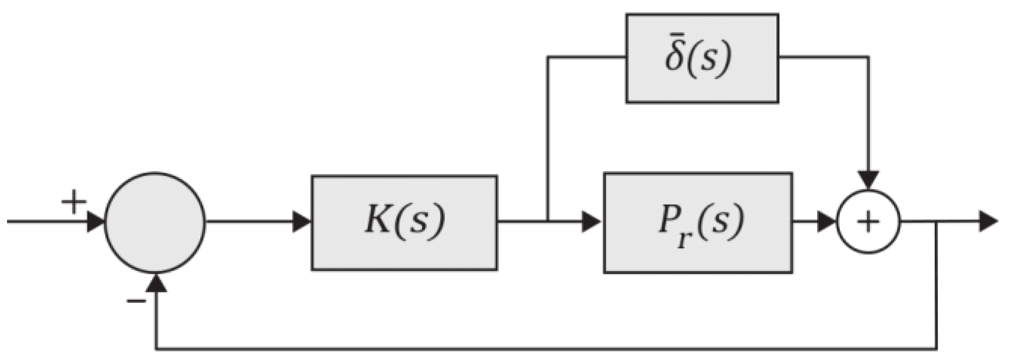
A order ROM of can be found such that has the same number of poles in the open right half plane as and is bounded on the imaginary axis. The closed-loop system with and is shown in Figure 2 where
and
is also a stabilizing controller for if
where
Again, the compensator reduction is a FWMOR problem, and thus can be reduced using cross-gramian -based FWMOR. Let’s take first, and can be achieved on similar lines by analogy. Let and be represented as the following state-space realizations, i.e.,
respectively. The augmented system is defined by
If is a symmetric system, its cross-gramian solves the following Sylvester Equation
can be partitioned according to , and the frequency-weighted can be extracted from as the block corressponding to in i.e.,
moreover, solves the following Sylvester Equations
Again, if is a non-symmetric system, the frequency-weighted cross-gramian can be obtained by either using the symmetrizer based approach of [10,11] or decentralized control based approach of [12]. Consider the symmetrizer-based approach first and let the eigenvalue decomposition of be . Then the frequency-weighted cross-gramian for the realization of can be computed by solving the following Sylvester Equation
where and .
If is not diagonalizable, the above-mentioned approach may not work. In that case, the decentralized control-based approach can be used to obtain the frequency-weighted cross-gramian , which solves the following Sylvester Equation
where and are the sums of the columns and rows of and , respectively.
Let be the transformation matrix, which diagonalizes such that eigenvalues are arranged according to their magnitude in descending order on the principal diagonal, i.e.,
where is an matrix. and can be partitioned as follows:
The ROM of can be computed as where
The proposed approach is summarized in Algorithm 1.
| Algorithm 1: Proposed Technique |
| Input: and . |
| Output: |
| 1: Select the desired loop TF such that has a high gain in the low-frequency region wherein disturbance attenuation is required, and a small gain in the high-frequency region wherein uncertainties in the plant are present. |
| 2: The desired closed-loop is . |
| 3: Initialize as . |
| 4: while , do set . |
| 5: Construct the augmented system from Equation (22). |
| 6: Compute from Equation (23). |
| 7: Compute from Equation (24). |
| 8: If is a SISO system, compute from Equation (25). |
| 9: If is a MIMO system, compute from Equations (26) or (27). |
| 10: Transform into ordered real Schur form i.e., |
| where is an matrix. |
| 11: Calculate the matrix by solving the following Sylvester Equation |
| . |
| 12: block diagonalises into . |
| 13: can be partitioned as . |
| 14: and . |
| 15: Compute using Equation (29). |
| 16: end while |
| 17: Design using any loop shaping technique such that the loop shape is achieved. |
| 18: If is a SISO system, compute from Equations (31), (32). |
| 19: If is a MIMO system, compute from Equation (33) or (34). |
| 20: Transform into ordered real Schur form |
| where is an matrix. |
| 21: Calculate the matrix by solving the following Sylvester Equation |
| 22: block diagonalizes into . |
| 23: can be partitioned as . |
| 24: and . |
| 25: Compute using Equation (36) such that . |
4. Numerical Examples
In this section, the proposed technique is validated on various benchmark control problems. The proposed algorithm is compared with EPRA [14] which is based on FWBT. We have changed the stopping criteria of EPRA to as in the proposed technique for a fair comparison. Furthermore, the controller obtained using EPRA is further reduced following the hybrid approach of the proposed algorithm for a fair comparison. The controllers are designed for the reduced plants using loop shaping procedure in References [24,25,26] and their loop shapes with the original plant are shown.
Example 1.
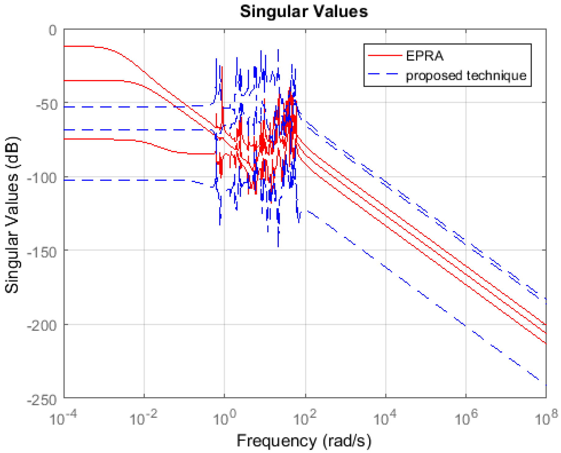
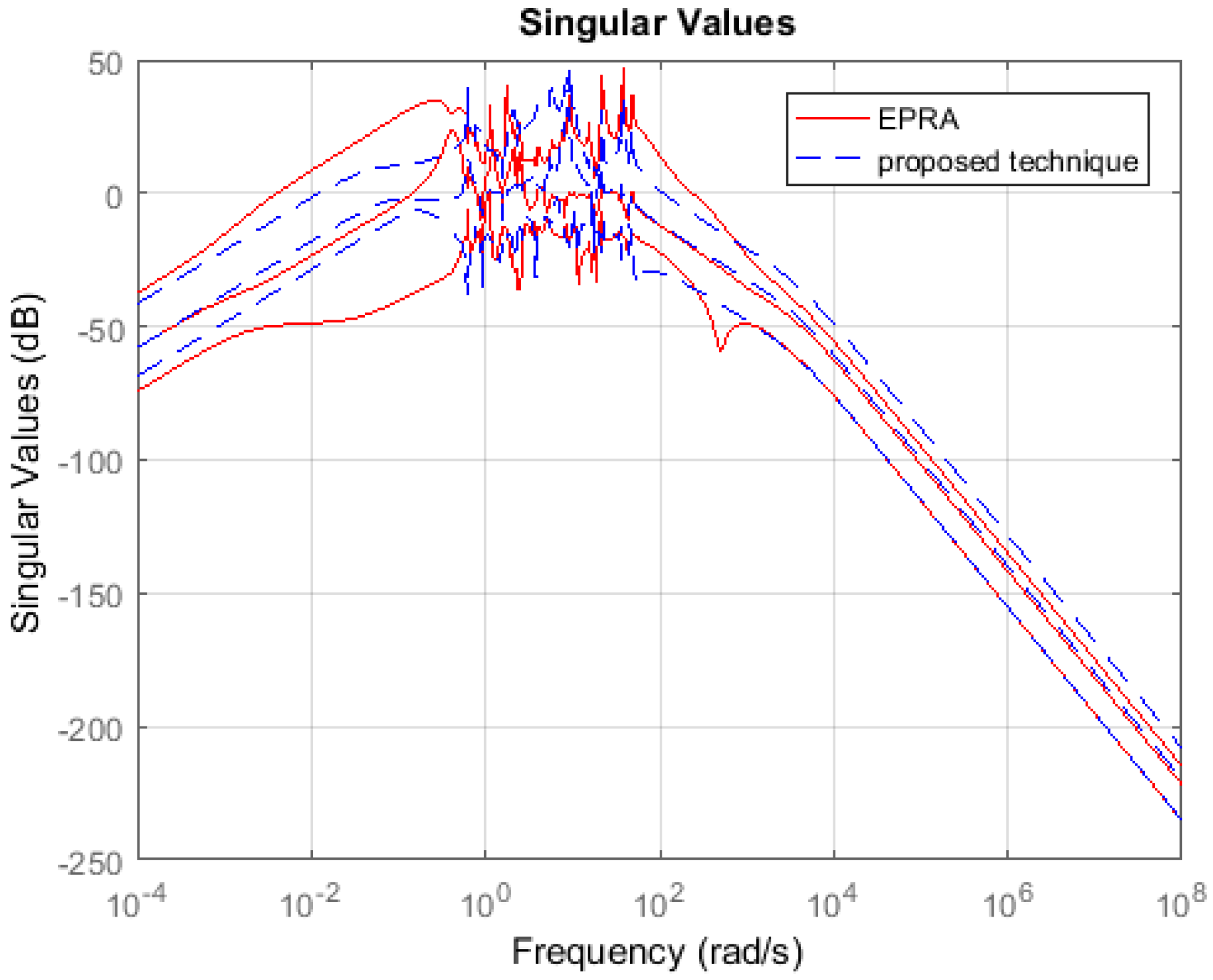
Symmetric System: Consider the 84th order SISO dynamic system represented by partial differential Equations taken from [27]. A 13th order reduced plant model is obtained using EPRA, and the proposed algorithm by setting . Table 1 shows a comparison between both techniques in terms of the weighted error . The simulation time in seconds yielded by both techniques are compared to check their computational efficiency. Figure 3 shows the weighted error . The controllers are designed for the reduced plants using the loop shaping procedure in [24,25,26]. Figure 4 shows the loop shape achieved using both techniques. The order of controllers obtained for 13 order reduced plants using EPRA, and the proposed algorithm is 14. The controller is further reduced to obtain a more compact controller of order 6 using FWBT and cross-gramian based FWMOR (steps 18–25 of Algorithm 1). Table 2 shows an error comparison in terms of weighted error for a 6th order controller. Figure 5 shows the weighted error . Figure 6 shows the loop shape achieved with this 6th order controller.
Example 2.
Non-symmetric System: Consider the international space station model in [27] which is a 270th order system with 3-inputs and 3-outputs. The model is a square but non-symmetric MIMO system. A 100th order reduced plant model is obtained using EPRA and Algorithm 1. Table 1 shows a comparison between both techniques in terms of the weighted error . The simulation time in seconds yielded by both techniques are compared to check their computational efficiency. Figure 7 shows the weighted error . The controllers are designed for the reduced plants using the loop shaping procedure in [24,25,26]. Figure 8 shows the loop shape achieved using both techniques. The orders of controllers obtained for 100th order reduced plants using EPRA and the proposed technique are 246 and 248, respectively. The controller is further reduced to obtain a more compact controller of order 20 using FWBT and cross-gramian based FWMOR (steps 18–25 of Algorithm 1). Table 2 shows an error comparison in terms of weighted error for the 20th order controller. Figure 9 shows the weighted error . Figure 10 shows the loop shape achieved with this 20th order controller.
Example 3.
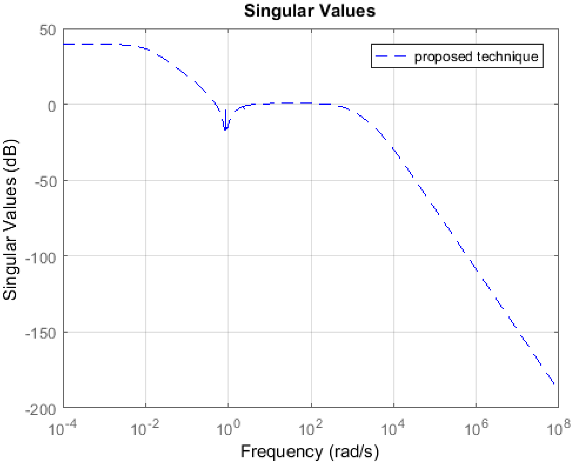
Unstable System: Consider an 8th order unstable model . Such that it contains a pair of eigenvalues (+1 and −1). Due to the presence of a set of eigenvalues with an equal magnitude but opposite sign, the solution of the standard Lyapunov and Sylvester Equation is not possible. Hence, well-known techniques such as [2,12,13,19] are not applicable to such systems. The proposed technique can be used to derive the 4th order reduced plant model (Algorithm 1). Table 1 shows the weighted error and simulation time in seconds yielded by the proposed technique. The controller is designed for the reduced plants using the loop shaping procedure in [24,25,26]. Figure 11 shows the loop shape achieved using the proposed technique. The order of controller obtained for 4th order reduced plant is 8. The controller is further reduced to obtain a more compact controller of order 5 using cross-gramian based FWMOR (steps 18–25 of Algorithm 1). Table 2 shows the weighted error for 5th order controller. Figure 12 shows the loop shape achieved with this 5th order controller.
5. Discussion
Table 1 and Table 2 show that the proposed algorithm is not only more accurate but also computationally efficient than EPRA. It can be seen from Figure 3 that the proposed technique is more accurate in the low and medium frequency region wherein the crossover frequencies lie. Figure 4 shows that the loop shape obtained for the 14th order controller using the proposed technique is similar to EPRA if not better. Additionally, it can be observed from Figure 6 that the controller obtained using the proposed algorithm exhibits a superior loop shape and good performance characteristics than EPRA despite being compact. In Example 2, the error yielded by the proposed technique is slightly more than EPRA, but still maintains its computational efficiency. Figure 7 shows the error comparison plot of the weighted error. Figure 8 shows that the loop shape obtained using the proposed technique is similar to EPRA if not better. A 20th order reduced controller is obtained for Example 2 using EPRA and proposed technique and the loop shape is shown in Figure 10. The weighted error is (as shown in Table 2), but still, a stabilizing controller is obtained where all the poles of the closed-loop system lie in the left half of s-plane. This is due to the fact that the satisfaction of criteria is a sufficient and not necessary condition for closed-loop stability. Analysis shows that if of order 184 is designed instead of 20 then the resulting stabilizing controllers obtained for EPRA and the proposed technique yield the weighted error 84.6631 and 0.1378 respectively. drastically increases after that, and the sufficient condition is not met. Since 184 is still a high order controller, we reduced the controller to 20th order and included the results for this controller. The performance of the reduced controller can be observed by the error analysis in Figure 5 and Figure 9, and it can be noted that the desired loop shape is acceptable. In Example 3, it is interesting to note that EPRA is not applicable, since the solution of standard Lyapunov Equations are not possible. However, by using the proposed technique, not only a stabilizing controller is obtained for the unstable plant, but also a much reduced/compact controller can be designed which preserves the closed-loop stability and performance criteria with the full order plant. Figure 11 and Figure 12 show the loop shape obtained using the proposed technique, and it can be noted that the loop gain is high in the low and medium frequency ranges.
6. Conclusions
In this paper, a controller reduction technique based on generalized frequency-weighted cross-gramian is proposed to design a compact reduced order controller for higher order plants. The scope of applicability is extended from stable SISO systems to unstable systems non-symmetric MIMO systems. The proposed algorithm does not require the original plant to be minimal, and it is computationally stable since a balancing free algorithm is used, which avoids ill-conditioning. The proposed algorithm yields a significantly lower-order controller for high order plants.
Author Contributions
The work furnished in this paper is a result of the mutual efforts of all authors. The guidance given by the second and fourth author has been greatly appreciated. Conceptualization, M.R.F.A., U.Z. and D.K.; Supervision, M.L.; Writing—original draft, M.R.F.A.
Funding
This research received no external funding.
Conflicts of Interest
The authors declare no conflict of interest.
References
- Li, Z.-H.; Chen, C.-J.; Teng, J.; Hu, W.-H.; Xing, H.-B.; Wang, Y. A Reduced-Order Controller Considering High-Order Modal Information of High-Rise Buildings for AMD Control System with Time-Delay. Shock Vib. 2017, 2017, 1–16. [Google Scholar] [CrossRef]
- Moore, B. Principal component analysis in linear systems: Controllability, observability, and model reduction. IEEE Trans. Autom. Control 1981, 26, 17–32. [Google Scholar] [CrossRef]
- Ghafoor, A.; Sreeram, V. A Survey/Review of Frequency-Weighted Balanced Model Reduction Techniques. J. Dyn. Syst. Meas. Control 2008, 130, 061004. [Google Scholar] [CrossRef]
- Safonov, M.G.; Chiang, R.Y. A Schur method for balanced-truncation model reduction. IEEE Trans. Autom. Control 1989, 34, 729–733. [Google Scholar] [CrossRef]
- Fernando, K.; Nicholson, H. On the structure of balanced and other principal representations of SISO systems. IEEE Trans. Autom. Control 1983, 28, 228–231. [Google Scholar] [CrossRef]
- Laub, A.J.; Silverman, L.M.; Verma, M. A note on cross-Grammians for symmetric realizations. Proc. IEEE 1983, 71, 904–905. [Google Scholar] [CrossRef]
- Fernando, K.; Nicholson, H. On the cross-Gramian for symmetric MIMO systems. IEEE Trans. Circuits Syst. 1985, 32, 487–489. [Google Scholar] [CrossRef]
- Zulfiqar, U.; Imran, M.; Ghafoor, A. Cross-Gramian based frequency-weighted model order reduction technique. Electron. Lett. 2016, 52, 1376–1377. [Google Scholar] [CrossRef]
- De Abreu-Garcia, J.; Fairman, F. A note on cross Grammians for orthogonally symmetric realizations. IEEE Trans. Autom. Control 1986, 31, 866–868. [Google Scholar] [CrossRef]
- Sorensen, D.C.; Antoulas, A.C. Projection Methods for Balanced Model Reduction. Available online: https://scholarship.rice.edu/handle/1911/101966 (accessed on 15 May 2019).
- Sorensen, D.C.; Antoulas, A.C. The Sylvester Equation and approximate balanced reduction. Linear Algebra Appl. 2002, 351–352, 671–700. [Google Scholar] [CrossRef]
- Himpe, C.; Ohlberger, M. A note on the cross Gramian for non-symmetric systems. Syst. Sci. Control Eng. 2016, 4, 199–208. [Google Scholar] [CrossRef] [Green Version]
- Aldhaheri, R.W. Model order reduction via real Schur-form decomposition. Int. J. Control 1991, 53, 709–716. [Google Scholar] [CrossRef]
- Enns, D.F. Model Reduction for Control System Design. Ph.D. Thesis, Stanford University, Stanford, CA, USA, 1984. Available online: https://ntrs.nasa.gov/search.jsp?R=19850014087 (accessed on 15 May 2019).
- Anderson, B.D.O.; Liu, Y. Controller reduction: Concepts and approaches. IEEE Trans. Autom. Control 1989, 34, 802–812. [Google Scholar] [CrossRef]
- Sanchez-Gasca, J.J.; Chow, J.H. Power system reduction to simplify the design of damping controllers for interarea oscillations. IEEE Trans. Power Syst. 1996, 11, 1342–1349. [Google Scholar] [CrossRef]
- Pal, B.; Chaudhuri, B. Robust Control in Power Systems; Power Electronics and Power Systems; Springer Science + Business Media: New York, NY, USA, 2005; ISBN 978-0-387-25949-9. [Google Scholar]
- Rogers, G. Power System Oscillations; Springer Science + Business Media: New York, NY, USA, 2000; ISBN 978-1-4613-7059-8. [Google Scholar]
- Enns, D. Model reduction with balanced realizations: An error bound and a frequency weighted generalization. In Proceedings of the 23rd IEEE Conference on Decision and Control, Las Vegas, NV, USA, 12–14 December 1984; IEEE: Las Vegas, NV, USA, 1984; pp. 127–132. [Google Scholar]
- Azhar, M.R.F.; Zulfiqar, U.; Liaquat, M. Cross-Gramian Based Lower-Order Controller Design. In Proceedings of the 6th International Conference on Control, Mechatronics and Automation (ICCMA 2018), Tokyo, Japan, 12–14 October 2018; ACM Press: Tokyo, Japan, 2018; pp. 53–59. [Google Scholar]
- Datta, K. The matrix Equation XA − BX = R and its applications. Linear Algebra Appl. 1988, 109, 91–105. [Google Scholar] [CrossRef]
- Zhou, K.; Salomon, G.; Wu, E. Balanced realization and model reduction for unstable systems. Int. J. Robust Nonlinear Control 1999, 9, 183–198. [Google Scholar] [CrossRef]
- Kumar, D.; Sreeram, V. Model Reduction via Generalized Frequency Interval Cross Gramian. IFAC-PapersOnLine 2018, 51, 25–29. [Google Scholar] [CrossRef]
- Le, V.X.; Safonov, M.G. Rational matrix GCDs and the design of squaring-down compensators-a state-space theory. IEEE Trans. Autom. Control 1992, 37, 384–392. [Google Scholar] [CrossRef]
- Glover, K.; McFarlane, D. Robust stabilization of normalized coprime factor plant descriptions with H/sub infinity/-bounded uncertainty. IEEE Trans. Autom. Control 1989, 34, 821–830. [Google Scholar] [CrossRef]
- Chiang, R.Y.; Safonov, M.G. H-infinity synthesis using a bilinear pole shifting transform. J. Guid. Control Dyn. 1992, 15, 1111–1117. [Google Scholar] [CrossRef]
- Chahlaoui, Y.; Van Dooren, P. Benchmark Examples for Model Reduction of Linear Time-Invariant Dynamical Systems. In Dimension Reduction of Large-Scale Systems; Benner, P., Sorensen, D.C., Mehrmann, V., Eds.; Springer: Berlin/Heidelberg, Germany, 2005; Volume 45, pp. 379–392. ISBN 978-3-540-24545-2. [Google Scholar]
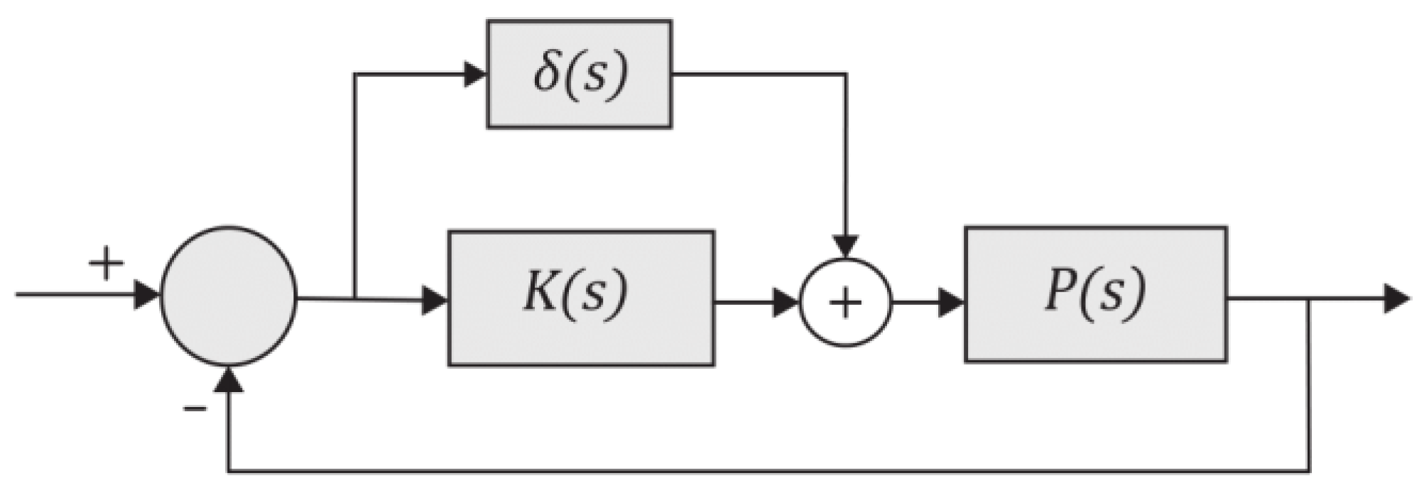
Figure 1.
Block diagram of closed-loop system [20].
Figure 1.
Block diagram of closed-loop system [20].

Figure 2.
Block diagram of closed-loop system [20].
Figure 2.
Block diagram of closed-loop system [20].

Figure 3.
Sigma plot of the weighted error .

Figure 4.
Sigma plot of .

Figure 5.
Sigma plot of the weighted error .

Figure 6.
Sigma plot of .

Figure 7.
Sigma plot of the weighted error .

Figure 8.
Sigma plot of .

Figure 9.
Sigma plot of the weighted error .

Figure 10.
Sigma plot of .

Figure 11.
Sigma plot of .

Figure 12.
Sigma plot of .


Table 1.
Comparison of weighted error and simulation time.
| Example | Order of | EPRA | Proposed Technique | ||
|---|---|---|---|---|---|
| Error | Time (s) | Error | Time (s) | ||
| 1 | 13 | 0.0010 | 0.0207 | 2.6 | 0.0097 |
| 2 | 100 | 0.2544 | 0.1269 | 0.4463 | 0.0481 |
| 3 | 4 | - | - | 0.5468 | 0.0003 |
Table 2.
Comparison of weighted error .
| Example | Order of | EPRA | Proposed Technique |
|---|---|---|---|
| 1 | 6 | 1.0009 | 3.0 |
| 2 | 20 | 4583.30 | 262.59 |
| 3 | 5 | - | 0.5676 |
© 2019 by the authors. Licensee MDPI, Basel, Switzerland. This article is an open access article distributed under the terms and conditions of the Creative Commons Attribution (CC BY) license (http://creativecommons.org/licenses/by/4.0/).
Share and Cite
MDPI and ACS Style
Azhar, M.R.F.; Zulfiqar, U.; Liaquat, M.; Kumar, D. Reduced Order Controller Design for Symmetric, Non-Symmetric and Unstable Systems Using Extended Cross-Gramian. Machines 2019, 7, 48. https://doi.org/10.3390/machines7030048
AMA Style
Azhar MRF, Zulfiqar U, Liaquat M, Kumar D. Reduced Order Controller Design for Symmetric, Non-Symmetric and Unstable Systems Using Extended Cross-Gramian. Machines. 2019; 7(3):48. https://doi.org/10.3390/machines7030048
Chicago/Turabian StyleAzhar, Muhammad Raees Furquan, Umair Zulfiqar, Muwahida Liaquat, and Deepak Kumar. 2019. "Reduced Order Controller Design for Symmetric, Non-Symmetric and Unstable Systems Using Extended Cross-Gramian" Machines 7, no. 3: 48. https://doi.org/10.3390/machines7030048
Note that from the first issue of 2016, this journal uses article numbers instead of page numbers. See further details here.