Changes in the Geographic Distribution of the Diana Fritillary (Speyeria diana: Nymphalidae) under Forecasted Predictions of Climate Change

1
Department of Biological Sciences, University of North Carolina at Charlotte, 9201 University City Blvd, Charlotte, NC 28223, USA
2
Department of Biology, University of Arkansas at Little Rock, 2801 South University Ave., Little Rock, AR 72204, USA
*
Author to whom correspondence should be addressed.
Insects 2018, 9(3), 94; https://doi.org/10.3390/insects9030094
Submission received: 2 July 2018
/
Revised: 20 July 2018
/
Accepted: 27 July 2018
/
Published: 2 August 2018
(This article belongs to the Special Issue Butterfly Ecology and Conservation)
Abstract
:Climate change is predicted to alter the geographic distribution of a wide variety of taxa, including butterfly species. Research has focused primarily on high latitude species in North America, with no known studies examining responses of taxa in the southeastern United States. The Diana fritillary (Speyeria diana) has experienced a recent range retraction in that region, disappearing from lowland sites and now persisting in two phylogenetically distinct high elevation populations. These findings are consistent with the predicted effects of a warming climate on numerous taxa, including other butterfly species in North America and Europe. We used ecological niche modeling to predict future changes to the distribution of S. diana under several climate models. To evaluate how climate change might influence the geographic distribution of this butterfly, we developed ecological niche models using Maxent. We used two global circulation models, the community climate system model (CCSM) and the model for interdisciplinary research on climate (MIROC), under low and high emissions scenarios to predict the future distribution of S. diana. Models were evaluated using the receiver operating characteristics area under curve (AUC) test and the true skill statistics (TSS) (mean AUC = 0.91 ± 0.0028 SE, TSS = 0.87 ± 0.0032 SE for representative concentration pathway (RCP) = 4.5; and mean AUC = 0.87 ± 0.0031 SE, TSS = 0.84 ± 0.0032 SE for RCP = 8.5), which both indicate that the models we produced were significantly better than random (0.5). The four modeled climate scenarios resulted in an average loss of 91% of suitable habitat for S. diana by 2050. Populations in the southern Appalachian Mountains were predicted to suffer the most severe fragmentation and reduction in suitable habitat, threatening an important source of genetic diversity for the species. The geographic and genetic isolation of populations in the west suggest that those populations are equally as vulnerable to decline in the future, warranting ongoing conservation of those populations as well. Our results suggest that the Diana fritillary is under threat of decline by 2050 across its entire distribution from climate change, and is likely to be negatively affected by other human-induced factors as well.
1. Introduction
Understanding how species distributions might shift with the changing climate is a critical component of managing and protecting future biodiversity. Hundreds of species in the United States and elsewhere have responded to the warming climate by shifting to higher latitudes or elevations [1,2,3,4]. Such range shifts have been documented in a number of taxa [5,6,7], including alpine plants [8], marine invertebrates [9], marine fish [10], mosquitoes [11], birds [12,13], and butterflies [1,14,15,16,17,18]. A number of species distribution models have been developed to predict the impacts of climate change on species distributions, including bioclimate envelope models, which are useful first estimates of the potential effects of climate change on altering species’ ranges [19]. Bioclimate envelope models work by identifying the climatic bounds within which a species currently occurs, and then delineating how those climatic bounds will shift under various future climate projections [20,21,22,23].
Most often, researchers are limited to presence-only occurrence data, requiring the use of indirect methods to infer a species’ climatic requirements [8,24,25]. One of the best performing models using presence-only data is maximum entropy modeling, or Maxent [26], which performs well even with low sample sizes typical of rare species [19,27,28]. Maxent works by comparing climate data from occurrence sites with those from a random sample of sites from the larger landscape to minimize the relative entropy of statistical models’ fit to each data set. Species distribution models such as Maxent have been criticized for being overly simplistic, because they do not incorporate external biotic factors such as species interactions [20,27,29]. However, such bioclimate envelope models have been used to project with reasonable accuracy whether species ranges will increase or decrease under a changing climate [19,30,31,32], which was the primary objective of this study.
Speyeria diana (Nymphalidae) (Cramer 1777) is a butterfly species endemic to the southeastern United States and is currently threatened across portions of its range. This species is of particular conservation interest because it has experienced a range collapse in recent decades resulting in an 800-km geographic and genetic disjunction between western populations in the Ouachita and Ozark Mountains and populations in the southern Appalachian Mountains, and has shifted to a higher elevation at an estimated rate of 18 m per decade [33]. This range contraction is consistent with the predicted effects of a warming climate, and might represent the first such documented case in the southeastern United States, though the region has experienced other environmental changes in recent decades as well [33]. Previous research using coalescent-based population divergence models dated the earliest splitting of the western population from the east at least 20,000 years ago, during the last glacial maximum [34]. In addition, recent geometric morphometric evidence from the wings of S. diana further support this long-term spatial and genetic isolation [35]. In light of these pieces of evidence, we used Maxent to model the future distribution of S. diana under several future climatic scenarios, in order to forecast how the range of the butterfly might shift under predicted conditions. Forecasts of large range reductions (over 50%), or small overlaps between current and future ranges (less than 50%), would suggest high vulnerability to climate change. Range reductions of any size in the western distribution would likely threaten those populations that are genetically isolated and adapted to relatively low dispersal, with the negative effects of genetic drift [34,35].
2. Methods
2.1. Study Species
The Diana fritillary, Speyeria diana, is a large and sexually dimorphic nymphalid butterfly, endemic to the southeastern United States. Adult males emerge in late May to early June, with females flying several weeks to a month later [36]. Once mated, each female can lay thousands of eggs singly on ground litter during the months of August and September in the vicinity of Viola spp., the larval host plant for all Speyeria [37]. After hatching, first instar larvae immediately burrow deep into the leaf litter layer of the forest floor, where they overwinter [38]. In spring, larvae feed on the foliage of freshly emerging violets. Adult Diana butterflies are often found along forest edges or dirt roads containing tall, conspicuous nectar sources such as milkweeds, butterfly bushes, or other large summer and fall composites [39,40,41,42]. While males begin to die off in late July, females may persist in large numbers, although somewhat cryptically, through October [42].
2.2. Distributional Dataset
We searched for all known records of S. diana, from publications, catalogued and uncatalogued specimens in public and private collections in the United States and Europe, online databases, contemporary field surveys by scientists and amateurs, and our own field surveys. We obtained distributional data from 1323 pinned S. diana specimens from 33 natural history museum collections in the United States and Europe (Table 1). Four hundred thirty-five additional records (1938–2012) were provided by the Butterfly and Moth Information Network and the participants who contribute to its BAMONA project. Our literature survey produced 153 records (1818–2011) across 54 U.S. counties (Table 2). We also collected 469 S. diana butterflies in our own field surveys (Table 3). Our dataset essentially represents a complete dataset of all publicly available records for the species, and is as comprehensive as for any taxon in the region [33]. For this reason, our dataset should be especially informative in creating an accurate bioclimate envelope for the species, as collection bias is a major consideration with ecological niche modeling [43,44].
2.3. Species Distributional Modeling
We developed species distribution models using the popular machine-learning algorithm for ecological modeling, Maxent [26]. Maxent estimates a species’ probability distribution that has maximum entropy (closest to uniform), subject to a set of constraints based on the sampling of presence-only data [45]. Because of the difficulty and impracticality of obtaining accurate absence data, presence-only data are most often used in species distribution modeling. In order to offset the lack of absence data, Maxent uses a background sample to compare the distribution of presence data along environmental gradients with the distribution of background points randomly drawn from the study area [46,47,48]. Locality data and the randomly sampled background points are combined with climatic data to predict the probability of the species’ occurrence within each raster grid cell. We used environmental climate data from WorldClim [49] at 30 arc-second resolution or approximately 1 km2 grid cells. Bioclimate variables and elevation layers were each clipped to the extent of North America using ESRI (Environmental Systems Research Institute) ArcMap 10.0, and data extracted to S. diana sample localities. Additionally, we collected the same types of locality data for three other species of North American butterflies (Speyeria cybele, Speyeria idalia, Battus philenor), which served as 5628 random background points for our models. We utilized these background data to minimize spatial bias in our modeling, as data represented by similar butterfly species can be used as pseudo-absence data with the same collection bias as our occurrence data, improving the accuracy of the model [50,51].
Climatic variables included 19 derived bioclimatic variables that describe annual and seasonal variation in temperature and precipitation, as well as elevation, averaged for 1950–2000 (Table 4). One concern when modeling species distributions is the strong correlation that occurs between multiple climate variables, which can significantly influence model predictions of species distributions [52]. To test for co-linearity, we performed spatial autocorrelation statistics between all pairs of the 19 bioclimate variables using ESRI ArcMap 10.0. We then selected the most biologically meaningful variable for each group of two or more variables with Pearson correlation coefficients higher than 0.7 (Table 4). This allowed us to reduce the number of bioclimate variables to the nine potentially most important ones, which were: Minimum Temperature of Coldest Month, Mean Temperature of Driest Quarter, Precipitation of Wettest Month, Precipitation of Driest Month, Precipitation of Driest Quarter, Isothermality, Mean Diurnal Range (Mean of monthly (maximum temperature—minimum temperature)), Temperature Annual Range, and Annual Precipitation, along with elevation (Table 4). These variables are typically considered to be important determinants of butterfly distributions, as they relate to life history traits. Butterflies are highly sensitive to weather and climate, particularly changes in temperature and rainfall [53]. For example, mean temperature of the coldest month is related to the overwintering survival of first instar larvae, growing degree days above 5 °C are regarded as a surrogate for the developmental threshold of the larvae, water balance corresponds to the moisture availability for the larval host and adult nectar plants, and the mean temperature of late summer ensures proper adult emergence and mating [54,55,56,57,58,59]. Temperature changes affect all aspects of butterfly life history, from their distribution and abundance [14,54], to their realized fecundity [60,61]. Changes in rainfall levels can influence butterfly larvae indirectly through changes in host plant quality, and generally rainfall is considered to be beneficial because it enhances host plant growth [62].
One concern when modeling species distributions is whether the occurrence records are spatially biased with respect to site accessibility (e.g., towns, roads, trails) [63]. To address this concern, we applied a spatial filter to remove all sampling points that were within 5 km of each other using ESRI ArcMap 10.0. The spatial filter resulted in 254 unique presence points for S. diana that were used in the final model. We first modeled the distribution of these 254 occurrences in present-day climate, and then projected the fitted species distribution under two future climate scenarios for the period 2040–2069 (hereafter referred to as 2050). Future climate scenarios were taken from two global circulation models (GCMs) obtained from www.worldclim.org; the community climate system model (CCSM) [64] and the model for interdisciplinary research on climate (MIROC) [65,66]. These GCMs differ in the reconstruction of several climatic variables and are well known to produce different outcomes for butterfly species [67,68]. For example, in hind-casting Mediterranean butterflies, the CCSM model projects narrower distributions at the last glacial maximum than does MIROC [65,66]. For each of these two GCMs, we considered two different representative concentration pathways (RCPs) [69,70,71,72,73], which are cumulative measures of human emissions of greenhouse gases from all sources expressed in Watts per square meter. These pathways were developed for the Fifth Assessment Report of the Intergovernmental Panel on Climate Change [67] and correspond to a total anthropogenic radiative forcing of RCP = 4.5 W/m2 (low) and RCP = 8.5 W/m2 (high) [72,73].
We used Maxent’s default parameters [26,50] and a ten-fold cross-validation approach to further reduce bias with respect to locality data. This method divides presence data into ten equal partitions, with nine used to train the model, and the tenth used to test it. These partitions generate ten maps (one map per run), with each raster grid cell containing a value representing the probability of occurrence. These values were used to designate habitat suitability ranging from 0 (unsuitable habitat) to 1 (highly suitable habitat) (Figure 1). We averaged the resulting maps for the current climate, and for the two GCMs under RCP = 4.5 and RCP = 8.5. This method resulted in the production of a “low” and “high” average prediction for S. diana species distribution in 2050, represented with habitat suitability maps. We measured the goodness of fit for the models using the area under the curve (AUC) of a receiver-operating characteristic (ROC) plot [74]. We used criteria of Swets [75] and considered AUC values higher than 0.7 representative of model predictions significantly better than random values of 0.5 or less [26,27,74]. Because AUC has been recognized as a somewhat questionable measure of accuracy, especially when used with background data instead of true absences [74,76], we also calculated the TSS (true skill statistics), a threshold-dependent evaluation metric [76,77]. The relative importance of each variable’s contribution was assessed by sequential variable removal by Jackknife [26].
3. Results
Species distributional modeling resulted in “excellent” model fits for Speyeria diana, with a mean AUC = 0.91 ± 0.0028 SE, TSS = 0.87 ± 0.0032 SE for RCP = 4.5; and a mean AUC = 0.87 ± 0.0031 SE, TSS = 0.84 ± 0.0032 SE for RCP = 8.5 (Table 1). Annual precipitation explained the largest fraction of the distribution of S. diana under both RCPs (17.9%, RCP = 4.5; 19.4%, RCP = 8.5). Among the remaining bioclimatic variables, mean temperature of driest quarter had the next highest average percent contribution (10.3%, RCP = 4.5; 25.0%, RCP = 8.5), followed by minimum temperature of coldest month (20.1%, RCP = 4.5; 10.4%, RCP = 8.5), isothermality (7.3%, RCP = 4.5; 7.6%, RCP = 8.5), precipitation of wettest month (3.5%, RCP = 4.5; 3.9%, RCP = 8.5), precipitation of driest month (1.4%, RCP = 4.5; 5.4%, RCP = 8.5), precipitation of driest quarter (3.3%, RCP = 4.5; 2.4%, RCP = 8.5), Elev (1.5%, RCP = 4.5; 3.5%, RCP = 8.5), mean diurnal range (1.8%, RCP = 4.5; 2.8%, RCP = 8.5), and temperature annual range (1.6%, RCP = 4.5; 1.3%, RCP = 8.5) (Table 1).
Modelling with Maxent under the selected climate-change scenarios predicted that habitat suitability would decrease for S. diana by 2050 (two-tailed paired t-tests comparing current Maxent values with those of 2050; all p < 0.01). The MIROC model resulted in more loss of suitable habitat than CCSM under both RCP scenarios (88.2% versus 92.4% of suitable habitat retained for RCP 4.5, and 90.2% versus 94.3% of suitable habitat retained for RCP 8.5 in CCSM and MIROC, respectively). Both climate models indicate that the loss of core distributional area is modest, with an average of 91.3% of present distributional areas retained. The most drastic reduction in habitat is apparent across the southern Appalachian Mountains (Figure 2).
4. Discussion
Our ecological niche models predicted that the amount of suitable habitat for Speyeria diana will decline substantially by the year 2050 across its entire distribution. Both CCSM and MIROC climate models predicted severe habitat loss and fragmentation in the southern Appalachian Mountains by 2050, with some range expansion predicted into higher latitudes in both eastern and western populations. High elevation habitat will be an important refuge for the species across the entire distribution, as the range of S. diana is already shifting to higher elevations at an estimated rate of 18 m per decade [33]. Recent evidence further suggests that some S. diana populations may already be adapting to high elevations, as S. diana female forewings from high elevation populations were found to be narrower than low elevation populations, indicating that these females may be more mobile than those from low elevations with wider forewings [35].
Unlike populations in the eastern distribution, the wing shape of western populations of S. diana appears to be better adapted for lower dispersal, which is in alignment with findings that western populations of S. diana are both spatially and genetically isolated [35]. Our models predicted that the southern edge of the highly suitable habitat in the west will recede by 2050; However, as was found in the southern Appalachian Mountains, the suitable habitat was predicted to expand in the higher elevations of the Ozark and Ouachita mountains of Arkansas. The genetic isolation of western populations may ultimately prevent them from adapting to higher elevations as successfully as populations in the eastern distribution of the species. If this is the case, lower elevation populations will be even more vulnerable to climate change than our models predict.
We would like to note that all ecological niche models should be used and interpreted with caution because of various sources of bias and error that result in inaccurate predictions [78]. Some have questioned the applicability of bioclimatic modeling at regional scales because of the somewhat coarse resolution [79]. However, we are confident that the size of our study area, and our uniquely extensive dataset, provide sufficient data to forecast climate-driven range shifts in S. diana with accuracy. Both global circulation models (CCCM and MIROC) were very closely aligned in their outcomes, indicating strong agreement between them. Climate is well understood to play a primary role in shaping the distributions of species [80], and we are confident in our overall findings that the suitable habitat for S. diana will decline and become increasingly fragmented by 2050.
5. Conclusions
These results highlight the importance of maintaining connectivity of the suitable habitat for S. diana, especially in the eastern populations that appear most vulnerable to increased fragmentation and loss of suitable habitat. These populations in the eastern distribution of S. diana harbor important genetic diversity that may become lost through genetic drift if these populations become small and isolated. The Ozark and Ouachita Mountains of Arkansas and Missouri appear to be least vulnerable to loss of suitable habitat from climate change, and therefore will be important for the future conservation of S. diana after 2050. As a result of the geographic and genetic isolation of the western populations, conservation of suitable habitat in the west is equally as important as in the east. Our climate models show that the 800-km disjunction across the center of the range of S. diana is not due to complete absence of suitable habitat, but more probably a result of the extensive habitat fragmentation regionally across the Ohio River Valley from agricultural land use change, and other human related factors that were not included in our models. We conclude that maintaining well-connected low and high elevation habitats across the entire distribution of S. diana, both now and into the future, will be necessary for this species, even under conservative forecasts of climate change.
Author Contributions
Conceptualization, D.T., C.N.W.; Methodology, C.N.W., D.T; Validation, C.N.W.; Formal Analysis, C.N.W.; Investigation, C.N.W.; Resources, C.N.W.; Data Curation, C.N.W, D.T.; Writing-Original Draft Preparation, C.N.W.; Writing-Review & Editing, D.T.; Visualization, C.N.W., D.T.; Supervision, D.T.; Project Administration, C.N.W.; Funding Acquisition, C.N.W., D.T.
Funding
This research received no external funding.
Acknowledgments
We would like to thank Kyle Barrett, and Sergio Marchant for their valuable assistance with this project. We also thank Peter Marko, Saara Dewalt, and Peter Adler for their careful reviews of this project and manuscript.
Conflicts of Interest
The authors declare no conflict of interest.
References
- Parmesan, C. Climate and species’ ranges. Nature 1996, 382, 765–766. [Google Scholar] [CrossRef]
- Parmesan, C.; Yohe, G. A globally coherent fingerprint of climate change impacts across natural systems. Nature 2003, 421, 37–42. [Google Scholar] [CrossRef] [PubMed]
- Thomas, C.D.; Franco, A.M.; Hill, J.K. Range retractions and extinction in the face of climate warming. Trends Ecol. Evol. 2004, 21, 415–416. [Google Scholar] [CrossRef] [PubMed]
- Crozier, L.; Dwyer, G. Combining population-dynamic and ecophysiological models to predict climate-induced insect range shifts. Am. Nat. 2006, 167, 853–866. [Google Scholar] [PubMed]
- Walther, G.R.; Post, E.; Convey, P.; Menzel, A.; Parmesan, C.; Beebee, T.; Fromentin, J.M.; Hoegh-Guldberg, O.; Bairlein, F. Ecological Responses to recent climate change. Nature 2002, 416, 389–395. [Google Scholar] [CrossRef] [PubMed]
- Root, T.L.; Price, J.T.; Hall, K.R.; Schneider, S.H.; Rosenzweig, C.; Pounds, J.A. Fingerprints of global warming on wild animals and plants. Nature 2003, 421, 57–60. [Google Scholar] [CrossRef] [PubMed]
- Parmesan, C. Ecological and evolutionary responses to recent climate change. Annu. Rev. Ecol. Evol. Syst. 2006, 37, 637–669. [Google Scholar] [CrossRef]
- Walther, G.R.; Beibner, S.; Conradin, A. Trends in the upward shift of alpine plants. J. Veg. Sci. 2005, 16, 541–548. [Google Scholar] [CrossRef] [Green Version]
- Cheung, W.W.L.; Lanm, W.Y.V.; Sarmiento, J.L.; Kearney, K.; Watson, R.; Pauly, D. Projecting global marine biodiversity impacts under climate change scenarios. Fish Fish. 2009, 10, 235–251. [Google Scholar] [CrossRef]
- Perry, A.L.; Low, P.J.; Ellis, J.R.; Reynolds, J.D. Climate change and distribution shifts in marine fishes. Science 2005, 308, 1912–1915. [Google Scholar] [CrossRef] [PubMed]
- Epstein, P.R.; Diaz, H.; Elias, F.S.; Grabherr, G.; Graham, N.E.; Martens, W.J.M.; Mosley-Thompson, E.; Susskind, E.J. Biological and physical signs of climate change: Focus on mosquito-borne disease. Bull. Am. Meteorol. Soc. 1998, 78, 409–417. [Google Scholar] [CrossRef]
- Thomas, C.D.; Lennon, J.J. Birds extend their ranges northwards. Nature 1999, 399, 213. [Google Scholar] [CrossRef]
- Hitch, A.T.; Leberg, P.L. Breeding distributions of North American bird species moving north as a result of climate change. Conserv. Biol. 2007, 21, 534–539. [Google Scholar] [CrossRef] [PubMed]
- Parmesan, C.; Ryrholm, N.; Stefanescu, C.; Hill, J.; Thomas, C.; Descimon, H.; Huntley, B.; Kaila, L.; Kullberg, J.; Tammaru, T.; et al. Poleward shifts in geographical ranges of butterfly species associated with regional warming. Nature 1999, 399, 579–583. [Google Scholar] [CrossRef]
- Wilson, R.J.; Gutiérrez, D.; Gutiérrez, J.; Martinez, D.; Aguado, R.; Monserrat, V.J. Changes to the elevational limits and extent of species ranges associated with climate change. Ecol. Lett. 2005, 8, 1138–1146. [Google Scholar] [CrossRef] [PubMed]
- Wilson, R.J.; Gutiérrez, D.; Gutiérrez, J.; Monserrat, V. An elevational shift in butterfly species richness and composition accompanying recent climate change. Glob. Chang. Biol. 2007, 13, 1873–1887. [Google Scholar] [CrossRef]
- Asher, J.; Fox, R.; Warren, M.S. British butterfly distributions and the 2010 target. J. Insect Conserv. 2011, 15, 291–299. [Google Scholar] [CrossRef]
- Wilson, R.J.; Maclean, I.M.D. Recent evidence for the climate threat to Lepidoptera and other insects. J. Insect Conserv. 2011, 15, 259–268. [Google Scholar] [CrossRef]
- Garcia, K.; Lasco, R.; Ines, A.; Lyon, B.; Pulhin, F. Predicting geographic distribution and habitat suitability due to climate change of selected threatened forest tree species in the Philippines. Appl. Geogr. 2013, 44, 12–22. [Google Scholar] [CrossRef]
- Pearson, R.G.; Dawson, T.P. Predicting the impacts of climate change on the distribution of species: Are bioclimate envelope models useful? Glob. Ecol. Biogeogr. 2003, 12, 361–371. [Google Scholar] [CrossRef]
- Peterson, A.T. Projected climate change effects on Rocky Mountain and Great Plain birds: Generalities on biodiversity consequences. Glob. Chang. Biol. 2003, 9, 647–655. [Google Scholar] [CrossRef]
- Elith, J.; Leathwick, J.R. Species distribution models: Ecological explanation and prediction across space and time. Annu. Rev. Ecol. Evol. Syst. 2009, 40, 677–697. [Google Scholar] [CrossRef]
- Fordham, D.A.; Resit, A.H.; Araújo, M.B.; Elith, J.; Keith, D.A.; Pearson, R.; Auld, T.D.; Mellin, C.; Morgan, J.W.; Regan, T.J.; et al. Plant extinction risk under climate change: Are forecast range shifts alone a good indicator of species vulnerability to global warming? Glob. Chang. Biol. 2012, 18, 1357–1371. [Google Scholar] [CrossRef]
- Thuiller, W.; Lavorel, S.; Araújo, M.B.; Sykes, M.T.; Prentice, I.C. Climate change threats to plant diversity in Europe. Proc. Natl. Acad. Sci. USA 2005, 102, 8245–8250. [Google Scholar] [CrossRef] [PubMed] [Green Version]
- Willis, K.J.; Araújo, M.B.; Bennett, K.D.; Figueroa-Range, B.; Froyd, C.A.; Myers, N. How can a knowledge of the past help to conserve the future? Biodiversity conservation and the relevance of long-term ecological studies. Philos. Trans. R. Soc. Lond. B Biol. Sci. 2007, 362, 175–186. [Google Scholar] [CrossRef] [PubMed]
- Phillips, S.J.; Anderson, R.; Schapire, R.E. Maximum entropy modeling of species geographic distributions. Ecol. Model. 2006, 190, 231–259. [Google Scholar] [CrossRef]
- Elith, J.; Phillips, S.J.; Hastie, T.; Dudík, M.; Chee, Y.E.; Yates, C.J. A statistical explanation of MaxEnt for ecologists. Divers. Distrib. 2011, 17, 43–57. [Google Scholar] [CrossRef]
- Weber, T.C. Maximum entropy modeling of mature hardwood forest distribution in four US states. For. Ecol. Manag. 2011, 261, 779–788. [Google Scholar] [CrossRef]
- Araújo, M.B.; Luoto, M. The importance of biotic interactions for modeling species distributions under climate change. Glob. Ecol. Biogeogr. 2007, 16, 743–753. [Google Scholar] [CrossRef]
- Araújo, M.B.; Pearson, R.G.; Thuiller, W.; Erhard, M. Validation of species-climate impact models under climate change. Glob. Chang. Biol. 2005, 11, 1504–1513. [Google Scholar] [CrossRef] [Green Version]
- Araújo, M.B.; Whittaker, R.J.; Ladle, R.J.; Erhard, M. Reducing uncertainty in projections of extinction risk from climate change. Glob. Ecol. Biogeogr. 2005, 14, 529–538. [Google Scholar] [CrossRef]
- Green, R.E.; Collingham, Y.C.; Willis, S.G.; Gregory, R.D.; Smith, K.W.; Huntley, B. Performance of climate envelope models in predicting recent changes in bird population size from observed climatic change. Biol. Lett. 2008, 4, 599–602. [Google Scholar] [CrossRef] [PubMed]
- Wells, C.N.; Tonkyn, D.W. Range collapse in the Diana fritillary, Speyeria diana (Nymphalidae). Insect Conserv. Divers. 2014, 7, 365–380. [Google Scholar] [CrossRef]
- Wells, C.N.; Marko, P.B.; Tonkyn, D.W. The phylogeographic history of the threatened Diana fritillary, Speyeria diana (Lepidoptera: Nymphalidae): With implications for conservation. Conserv. Genet. 2015, 16, 703–716. [Google Scholar] [CrossRef]
- Wells, C.N.; Munn, A.; Woodworth, C. Geomorphic Morphometric Differences between Populations of Speyeria diana (Lepidoptera: Nymphalidae). Fla. Entomol. 2018, 101, 195–202. [Google Scholar] [CrossRef]
- Opler, P.A.; Krizek, G. Butterflies East of the Great Plains; Johns Hopkins University Press: Baltimore, MD, USA, 1984; p. 294. ISBN 0801829380. [Google Scholar]
- Allen, T.J. The Butterflies of West Virginia and their Caterpillars; University of Pittsburgh Press: Pittsburgh, PA, USA, 1997; p. 388. ISBN 0822939738. [Google Scholar]
- Cech, R.; Tudor, G. Butterflies of the East Coast; Princeton University Press: Princeton, NJ, USA, 2005; p. 345. ISBN 069109055. [Google Scholar]
- Baltosser, W. Flitting with disaster: Humans and habitat are keys to our state butterfly’s future. Ark. Wildl. 2007, 38, 6–11. [Google Scholar]
- Ross, G.N. What’s for dinner? A new look at the role of phytochemicals in butterfly diets. News Lepidopterists’ Soc. 2003, 45, 83–89. [Google Scholar]
- Ross, G.N. Diana’s Mountain Retreat. Nat. Hist. 2008, 72, 24–28. [Google Scholar]
- Adams, J.K.; Finkelstein, I. Late season observations on female Diana fritillary (Speyeria diana) aggregating behavior. News Lepidopterists’ Soc. 2006, 48, 106–107. [Google Scholar]
- Araújo, M.B.; Peterson, A.T. Uses and misuses of bioclimatic envelope modeling. Ecology 2012, 93, 1527–1539. [Google Scholar] [CrossRef] [PubMed] [Green Version]
- Loiselle, B.A.; Jørgensen, P.M.; Consiglio, T.; Jiménez, I.; Blake, J.G.; Lohmann, L.G.; Montiel, O.M. Predicting species distributions from herbarium collections: Does climate bias in collection sampling influence model outcomes? J. Biogeogr. 2007, 35, 105–116. [Google Scholar] [CrossRef]
- Renner, I.W.; Warton, D.I. Equivalence of MAXENT and Poisson Point Process Models for Species Distribution Modeling in Ecology. Biometrics 2013, 69, 274–281. [Google Scholar] [CrossRef] [PubMed]
- Gomes, V.H.F.; Jff, S.D.I.; Raes, N.; Amaral, I.L.; Salomão, R.P.; Coelho, L.d.; Matos, F.D.d.A.; Castilho, C.V.; Filho, D.d.L.; López, D.C.; et al. Species Distribution Modelling: Contrasting presence-only models with plot abundance data. Sci. Rep. 2018, 8, 1003. [Google Scholar] [CrossRef] [PubMed] [Green Version]
- Elith, J.; Graham, C.H. NCEAS Species Distribution Modelling Group, Novel methods improve prediction of species’ distributions from occurrence data. Ecography 2006, 29, 129–151. [Google Scholar] [CrossRef]
- Elith, J.; Kearney, M.; Phillips, S. The art of modeling range-shifting species. Methods Ecol. Evol. 2010, 1, 330–342. [Google Scholar] [CrossRef]
- Hijmans, R.J.; Cameron, S.E.; Parra, J.L.; Jones, P.G.; Jarvis, A. Very high resolution interpolated climate surfaces for global land areas. Int. J. Climatol. 2005, 25, 1965–1978. [Google Scholar] [CrossRef] [Green Version]
- Phillips, S.J.; Dudík, M. Modeling of species distributions with Maxent: New extensions and a comprehensive evaluation. Ecography 2008, 31, 161–175. [Google Scholar] [CrossRef]
- Phillips, S.J.; Dudík, M.; Elith, J.; Graham, C.H.; Lehmann, A.; Leathwick, J.; Ferrier, S. Sample selection bias and presence-only distribution models: Implications for background and pseudo-absence data. Ecol. Appl. 2009, 19, 181–197. [Google Scholar] [CrossRef] [PubMed]
- Beaumont, L.; Hughes, L.; Poulsen, M. Predicting species distributions: Use of climatic parameters in BIOCLIM and its impact on predictions of species’ current and future distributions. Ecol. Model. 2005, 186, 250–269. [Google Scholar] [CrossRef]
- Dennis, R.L.H. Butterflies and Climate Change; Manchester University Press: Manchester, UK, 1993. [Google Scholar]
- Hill, J.K.; Thomas, C.D.; Huntley, B. Modelling present and potential future ranges of European butterflies using climate response surfaces. In Butterflies: Ecology and Evolution Taking Flight; Boggs, C.L., Watt, W.B., Ehrlich, P.R., Eds.; University of Chicago Press: Chicago, IL, USA, 2003; pp. 149–167. [Google Scholar]
- Peterson, A.T.; Martínez-Meyer, E.; González-Salazar, C.; Hall, P.W. Modeled climate change effects on distributions of Canadian butterfly species. Can. J. Zool. 2004, 82, 851–858. [Google Scholar] [CrossRef] [Green Version]
- Mitikka, V.; Heikkinen, R.K.; Luoto, M.; Araújo, M.B.; Saarinen, K.; Pöyry, J.; Fronzek, S. Predicting range expansion of the map butterfly in Northern Europe using bioclimatic models. Biodivers. Conserv. 2008, 17, 623–641. [Google Scholar] [CrossRef]
- Filz, K.J.; Schmitt, T.; Engler, J.O. How fine is fine-scale? Questioning the use of fine-scale bioclimatic data in species distribution models used for forecasting abundance patterns in butterflies. Eur. J. Entomol. 2013, 110, 311–317. [Google Scholar] [CrossRef] [Green Version]
- Zinetti, F.; Dapporto, L.; Vovlas, A.; Chelazzi, G.; Bonelli, S.; Balletto, E.; Ciofi, C. When the rule becomes the exception: No evidence of gene flow between two Zerynthia cryptic butterflies suggests the emergence of a new model group. PLoS ONE 2013, 8, e65746. [Google Scholar] [CrossRef] [PubMed]
- Hill, J.K.; Thomas, C.D.; Fox, R.; Telfer, M.G.; Willis, S.G.; Asher, J.; Huntley, B. Responses of butterflies to twentieth century climate warming: Implications for future ranges. Proc. R. Soc. Lond. Ser. B Biol. Sci. 2002, 269, 2163–2171. [Google Scholar] [CrossRef] [PubMed] [Green Version]
- Karlsson, B.; Van Dyck, H. Does habitat fragmentation affect temperature-related life-history traits? A laboratory test with a woodland butterfly. Proc. R. Soc. Lond. Ser. B Biol. Sci. 2005, 272, 1257–1263. [Google Scholar] [CrossRef] [PubMed] [Green Version]
- Gibbs, M.; Van Dyck, H.; Karlsson, B. Reproductive plasticity, ovarian dynamics and maternal effects in response to temperature and flight in Pararge aegeria. J. Insect Physiol. 2010, 56, 1275–1283. [Google Scholar] [CrossRef] [PubMed]
- Morecroft, M.D.; Bealey, C.E.; Howells, O.; Rennie, S.; Woiwod, I.P. Effects of drought on contrasting insect and plant species in the UK in the mid-1990s. Glob. Ecol. Biogeogr. 2002, 11, 7–22. [Google Scholar] [CrossRef]
- Kadmon, R.; Farbr, O.; Danin, A. Effect of roadside bias on the accuracy of predictive maps produced by bioclimatic models. Ecol. Appl. 2004, 14, 401–413. [Google Scholar] [CrossRef]
- Gent, P.R.; Danabasoglu, G.; Donner, L.J.; Holland, M.M.; Hunke, E.C.; Jayne, S.R.; Lawrence, D.M.; Neale, R.B.; Rasch, P.J.; Vertenstein, M.; et al. The community climate system model, Version 4. J. Clim. 2011, 24, 4973–4991. [Google Scholar] [CrossRef]
- Hasumi, H.; Emori, S. K-1 Coupled GCM (MIROC) Description; K-1 Tech. Rep. 1; Center for Climate Systems Research, University of Tokyo: Tokyo, Japan, 2004; p. 34. [Google Scholar]
- Nozawa, T.; Nagashima, T.; Shiogama, H.; Crooks, S.A. Detecting natural influence on surface air temperature change in the early twentieth century. Geophys. Res. Lett. 2005, 32, L20719. [Google Scholar] [CrossRef]
- Habel, J.C.; Rödder, D.; Scalercio, S.; Meyer, M.; Schmitt, T. Strong genetic cohesiveness between Italy and North Africa in four butterfly species. Biol. J. Linn. Soc. 2010, 99, 818–830. [Google Scholar] [CrossRef] [Green Version]
- Habel, J.C.; Husemann, M.; Schmitt, T.; Dapporto, L.; Vandewoestijne, S. A forest butterfly in Sahara desert oases: Isolation does not matter. J. Hered. 2013, 104, 234–247. [Google Scholar] [CrossRef] [PubMed]
- Moss, R.H.; Edmonds, J.A.; Hibbard, K.A.; Manning, M.R.; Rose, S.K.; van Vuuren, D.P.; Carter, T.R.; Emori, S.; Kainuma, M.; Kram, T.; et al. The next generation of scenarios for climate change research and assessment. Nature 2010, 463, 747–756. [Google Scholar] [CrossRef] [PubMed]
- Van Vuuren, D.P.; Edmonds, J.; Kainuma, M.; Riahi, K.; Thomson, A.; Hibbard, K.; Hurtt, G.C.; Kram, T.; Krey, V.; Lamarque, J.F.; et al. The representative concentration pathways: An overview. Clim. Chang. 2011, 109, 5–31. [Google Scholar] [CrossRef]
- Moss, R.H.; Babiker, M.; Brinkman, S.; Calvo, E.; Carter, T.; Edmonds, J.; Elgizouli, I.; Emori, S.; Erda, L.; Hibbard, K.; et al. Towards New Scenarios for Analysis of Emissions, Climate Change, Impacts, and Response Strategies; Intergovernmental Panel on Climate Change: Geneva, Switzerland, 2008; p. 132. [Google Scholar]
- Riahi, K.; Rao, S.; Krey, V.; Cho, C.; Chirkov, V.; Fischer, G.; Kindermann, G.; Nakicenovic, N.; Rafaj, P. RCP 8.5—A scenario of comparatively high greenhouse gas emissions. Clim. Chang. 2011, 109, 33–57. [Google Scholar] [CrossRef] [Green Version]
- Thomson, A.; Calvin, K.; Smith, S.; Kyle, P.; Volke, A.; Patel, P.; Delgado-Arias, S.; Bond-Lamberty, B.; Wise, M.; Clarke, L.; et al. RCP4.5: A pathway for stabilization of radiative forcing by 2100. Clim. Chang. 2011, 109, 77–94. [Google Scholar] [CrossRef]
- Jiménez-Valverde, A. Insights into the area under the receiver operating characteristic curve (AUC) as a discrimination measure in species distribution modelling. Glob. Ecol. Biogeogr. 2012, 21, 498–507. [Google Scholar] [CrossRef]
- Swets, J.A. Measuring the accuracy of diagnostic systems. Science 1988, 240, 1285–1293. [Google Scholar] [CrossRef] [PubMed]
- Allouche, O.; Tsoar, A.; Kadmon, R. Assessing the accuracy of species distribution models: Prevalence, kappa and the true skill statistic (TSS). J. Appl. Ecol. 2006, 43, 1223–1232. [Google Scholar] [CrossRef]
- Fielding, A.H.; Bell, J.F. A review of methods for the assessment of prediction errors in conservation presence/absence models. Environ. Conserv. 1997, 24, 38–49. [Google Scholar] [CrossRef]
- Beaumont, L.J.; Hughes, L.; Pitman, A.J. Why is the choice of future climate scenarios for species distribution modelling important? Ecol. Lett. 2008, 11, 1135–1146. [Google Scholar] [CrossRef] [PubMed] [Green Version]
- Chen, I.C.; Hill, J.K.; Ohlemuller, R.; Roy, D.B.; Thomas, C.D. Rapid range shifts of species associated with high levels of climate warming. Science 2011, 333, 1024–1026. [Google Scholar] [CrossRef] [PubMed]
- Fourcade, Y.; Besnard, A.G.; Secondi, J. Paintings predict the distribution of species, or the challenge of selecting environmental predictors and evaluation statistics. Glob. Ecol. Biogeogr. 2018, 27, 245–256. [Google Scholar] [CrossRef]
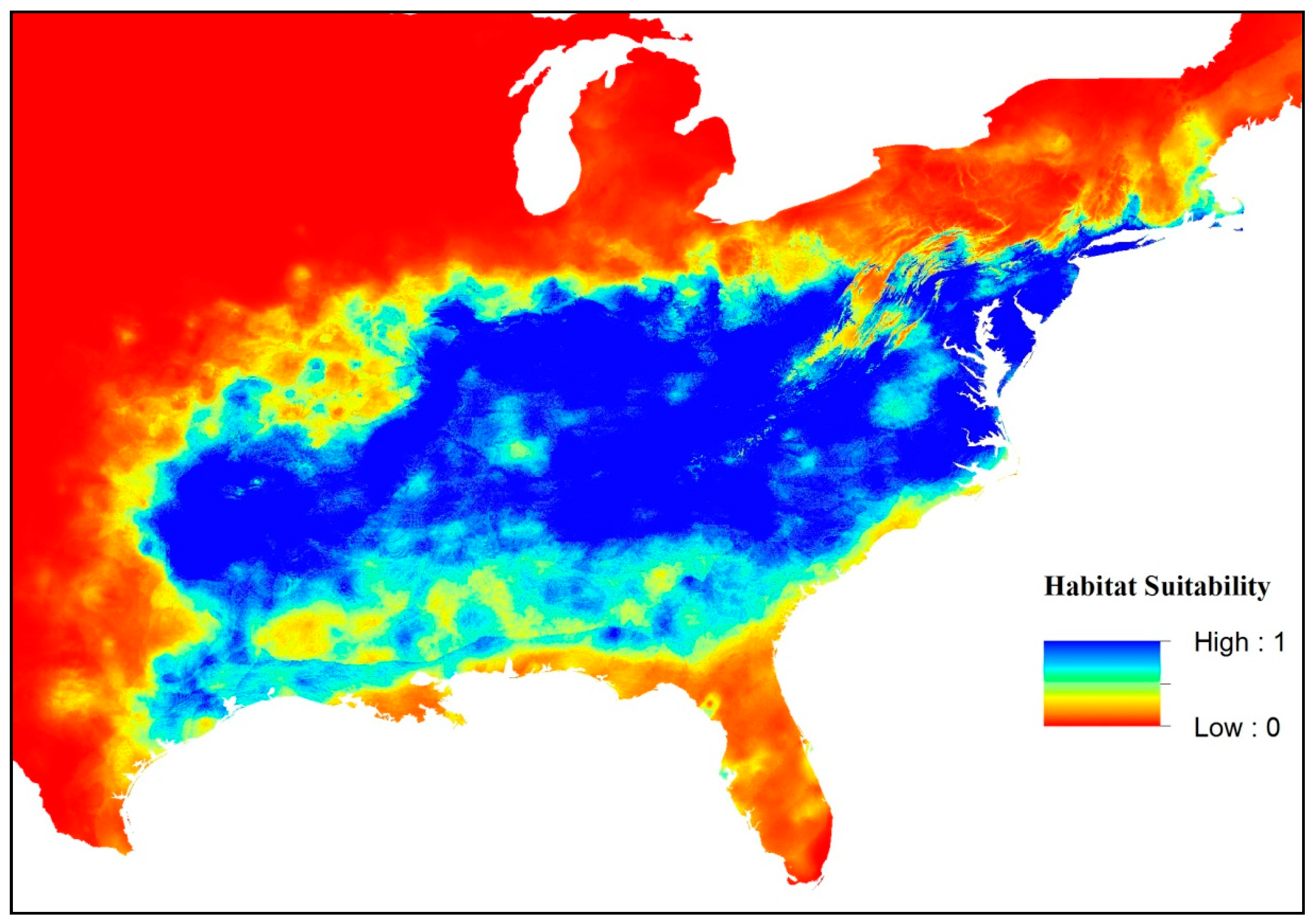
Figure 1.
The present-day geographic distribution of Speyeria diana, with indices of habitat suitability as predicted by maximum entropy modelling (Maxent) under current climatic conditions (1950–2010).
Figure 1.
The present-day geographic distribution of Speyeria diana, with indices of habitat suitability as predicted by maximum entropy modelling (Maxent) under current climatic conditions (1950–2010).

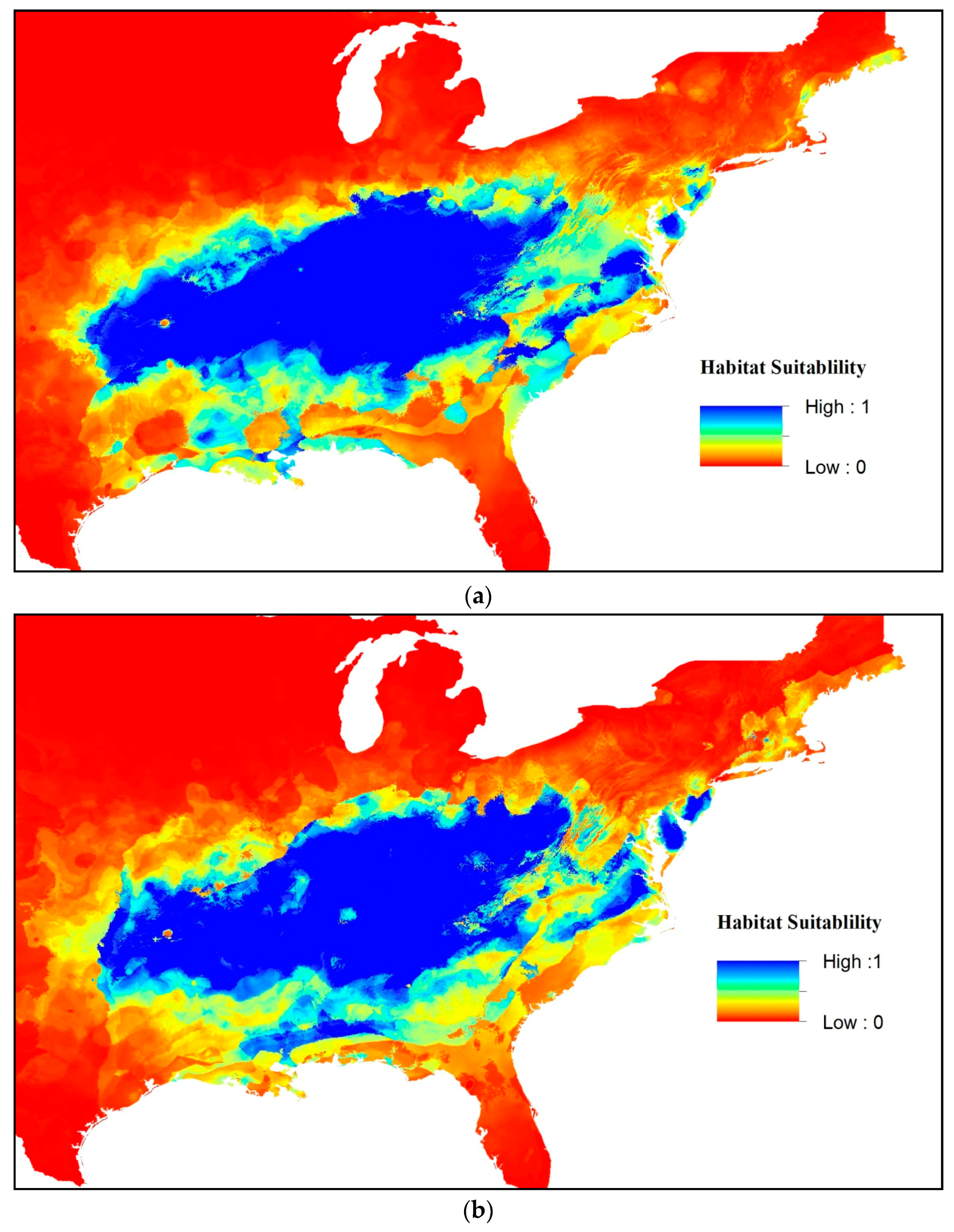
Figure 2.
(a) Habitat suitability indices for the projected future distribution of Speyeria diana under the community climate system model (CCMA) and model for interdisciplinary research on climate (MIROC) representative concentration pathways (RCP) 4.5 climate change scenarios; (b) habitat suitability indices for the projected future distribution of Speyeria diana under the CCMA and MIROC RCP 8.5 climate change scenarios.


Table 1.
Summary of Speyeria diana distributional data sources (adapted from Wells and Tonkyn 2014).
Table 1.
Summary of Speyeria diana distributional data sources (adapted from Wells and Tonkyn 2014).
| National Museums (N. American) | Location | No. of S. diana | Range of Specimen Dates | No. of Counties |
|---|---|---|---|---|
| Carnegie Museum of Natural History | Pittsburgh, Pennsylvania | 142 | 1889–2000 | 26 |
| National Museum of Natural History | Washington, DC | 129 | 1907–2002 | 26 |
| American Museum of Natural History | New York, NY | 104 | 1921–1985 | 28 |
| The Field Museum | Chicago, IL | 98 | 1889–1995 | 23 |
| California Academy of Sciences | San Francisco, CA | 88 | 1886–2000 | 12 |
| Georgia Museum of Natural History | Athens, GA | 15 | 1935–1987 | 8 |
| Cleveland Museum of Natural History | Cleveland, Ohio | 6 | 1921–1965 | 6 |
| Denver Museum of Nature and Science | Denver, Colorado | 4 | 1939–1973 | 3 |
| Mount Magazine State Park | Paris, Arkansas | 4 | 1997 | 1 |
| National History Museums (European) | ||||
| British Natural History Museum | London, UK | 31 | 1777–1989 | 17 |
| Paris Muséum national d’Histoire naturelle | Paris, France | 8 | 1890 | 1 |
| Oxford Museum of Natural History | Oxford, UK | 4 | 1937–1971 | 4 |
| Zoölogisch Museum Amsterdam | Amsterdam, The Netherlands | 4 | 1884–1921 | 3 |
| Naturalis Biodiversity Center | Leiden, Netherlands | 4 | ||
| Royal Ontario Museum | Ontario, Canada | 3 | 1933–1968 | 3 |
| University Collections | ||||
| University of Florida | Gainesville, Florida | 409 | 1900–2007 | 43 |
| University of Michigan | East Lansing, Michigan | 66 | 1909–1985 | 13 |
| Clemson University | Clemson, South Carolina | 43 | 1926–1978 | 5 |
| Peabody, Yale University | New Haven, Connecticut | 29 | 1904–1961 | 8 |
| University of Missouri | Columbia, Missouri | 29 | 1886–1980 | 8 |
| University of Wyoming | Laramie, Wyoming | 13 | 1955–1979 | 4 |
| University of Arkansas, Little Rock | Little Rock, Arkansas | 12 | 2005–2007 | 5 |
| University of California, Berkley | Berkley, California | 12 | 1926–1981 | 6 |
| University of Nebraska | Lincoln, Nebraska | 14 | 1954–2003 | 7 |
| North Carolina State University | Raleigh, North Carolina | 10 | 1904–1964 | 9 |
| University of Arkansas, Fayetteville | Fayetteville, Arkansas | 10 | 1977–1994 | 5 |
| Virginia Polytechnic Inst | Blacksburg, Virginia | 8 | 1911–1977 | 1 |
| Louisiana State University | Baton Rouge, Louisiana | 7 | 1984–1988 | 1 |
| University of Wisconsin | Madison, WI | 5 | 1926–1951 | 2 |
| College of Charleston | Charleston, South Carolina | 4 | 2008 | 2 |
| West Virginia University | Morgontown, West Virginia | 3 | 1977–1995 | 2 |
| Furman University | Greenville, South Carolina | 3 | 1929–1990 | 3 |
| Dalton State College | Dalton, Georgia | 2 | 2001 | 1 |
| State Agencies, online databases, listserves, individuals, and organizations | ||||
| Field Surveys | 469 | 1995–2012 | 46 | |
| Butterflies and Moths of America (BAMONA) | 435 | 1938–2012 | 39 | |
| North Carolina 19th Approximation (http://149.168.1.196/nbnc/) | 276 | 1938–2011 | 31 | |
| West Virginia Divisions of Natural Resources (wvdnr.gov) | 204 | 1978–1999 | 11 | |
| Literature survey | 153 | 1818–2011 | 54 | |
| Kentucky Dept. of Fish and Wildlife Resources (fw.ky.gov) | 146 | 1936–2006 | 21 | |
| NABA annual count data (naba.org) | 103 | 1999–2010 | 27 | |
| Georgia Dept. of Natural Resources (gadnr.org) | 77 | 1994–2001 | 15 | |
| Global Biodiversity Information Facility (GBIF) | 75 | 1974–2004 | 49 | |
| North Carolina Natural Heritage Program (nchp.org) | 69 | 1989–2003 | 21 | |
| The Lepidopterists’ Society (lepsoc.org) | 50 | 1973–2008 | 25 | |
| All Taxa Biodiversity Inventory (ATBI) (dlia.org/atbi) | 46 | 1936–2007 | 4 | |
| Carolina Butterfly Society (CBS) | 44 | 2001–2009 | 5 | |
| Carolinaleps | 41 | 2007–2009 | 9 | |
| Washington Area Butterfly Club | 29 | 2007 | 1 | |
| Oklahoma Leps | 21 | 2005–2009 | 5 | |
| Insect.net | 21 | 2007–2009 | 9 | |
Table 2.
Summary of literature referencing the distribution of Speyeria diana (adapted from Wells and Tonkyn 2014).
Table 2.
Summary of literature referencing the distribution of Speyeria diana (adapted from Wells and Tonkyn 2014).
| Reference | Location | Date of Record(s) | Description |
|---|---|---|---|
| Cramer & Stoll 1775 | Jamestown, Virginia | 1775 | holotype; male described by Pieter Cramer |
| Blatchley 1859 | Vanderburgh County, Indiana | 1850s | first record from Indiana, most northern record |
| Edwards 1864 | Kanawha, West Virginia | 20–31 August 1864 | first description of female, took over 30 specimens |
| Edwards 1874 | Coalburgh, West Virginia | August, September 1873 | description of rearing Argynnis larvae |
| Aaron 1877 | Tennessee/North Carolina | 1877 | populations are ample along Blue Ridge |
| Kentucky | 1877 | locally abundant populations | |
| Strecker 1878 | 1878 | West Virginia, Georgia, Kentucky, Tennessee, Arkansas | |
| Thomas 1878 | Kentucky, Arkansas, southern Illinois | 1878 | common in Kentucky & Arkansas |
| Fisher 1881 | Illinois | 1880 | present in southern Illinois |
| Holland 1883 | Salem, North Carolina | 1858–1861 | described as “first pinned female specimen” |
| Edwards 1884 | southern Ohio | 1880s | first description in Ohio |
| Hulst 1885 | Waynesville, North Carolina | 1882 | locally abundant populations |
| Warren Springs, North Carolina | 1882 | very common along the French Broad River | |
| Blatchley 1886 | Evansville, Indiana | early 1900s | locally abundant populations |
| French 1886 | eastern United States | 1886 | W. Virginia to Georgia, Southern Ohio to Illinois, Kentucky, Tennessee, Arkansas |
| Hine 1887a, b | Medina County, Ohio | 9 August 1887 | single worn male, northernmost record in OH |
| Kingsley 1888 | Virginia | 1887 | Argynnis diana is described as the handsomest insect found in the United States |
| Scudder 1889 | southeast United States | 1880s | Semnopsyche diana; an inhabitant of hilly country of the south, 38th parallel of latitude, taken as far west as Missouri and “Arkansaw” |
| Skinner & Aaron 1889 | Pennsylvania | 1880s | stray individual found in Pennsylvania |
| Dixey 1890 | eastern United States | 1889 | description of Argynnis diana wing spot pattern |
| Blatchley 1891 | Illinois | 1890s | female specimen from northern Danville, IL |
| Skinner 1896 | southern Illinois | 1890s | Diana specimens from southern Illinois are larger than those further east |
| Holland 1898 | southern United States | 1890s | in two Virginias and Carolinas, northern Georgia, Tennessee, Kentucky, occasionally in southern Ohio and Indiana, and in Missouri and Arkansas; the most magnificent and splendid species of the genus |
| Snyder 1900 | Clay County, Illinois | 1900 | northern limit of S. diana in Illinois |
| Strecker 1900 | Missouri | 1853 | pair captured in copula, very early female |
| Maynard 1901 | habitat is West Virginia to Georgia, southern Ohio to Illinois, Tennessee, and Arkansas | ||
| Sell 1916 | Greene County, Missouri | 22 August 1900 | southeast of Springfield |
| Smyth 1916 | southeast United States | 1880–1916 | Asheville, Brevard, North Carolina, Caesar’s Head, South Carolina, Montgomery, Washington and Giles Counties, Virginia |
| Wood 1916 | Camp Craig, Virginia | August 1914 | describes female color variation |
| Murrill 1919 | Virginia | 1919 | Poverty Valley |
| Holland 1931 | 1930s | The Virginias and Carolinas, northern GA Tennessee, Kentucky, occasionally in southern OH, Indiana, and in Missouri and Arkansas | |
| Knobel 1931 | Hope, Arkansas | 1930 | from Mrs. Louise Knobel |
| Kite 1934 | Taney County, Missouri | 31 July 1925 | male and female reported |
| Clark 1937 | Virginia | 1930s | ranges from Bath County, Virginia to FL east almost to tidewater, and west to Illinois and Arkansas |
| Clark & Williams 1937 | Virginia | late 1800s–1935 | Bath, Alleghany, Giles, Bland, Dickenson, Smyth, Patrick, Montgomery & Washington Counties |
| Allen 1941 | West Virginia | 1940 | Pocahontas County, west to Kanawha and Lincoln Counties; abundant in Jefferson NF (Monroe County), Babcock State Park (Fayette County), and Fork Creek Wildlife Management Area (Boone County) |
| Chermock 1942 | Conestee Falls, North Carolina | summer 1941 | southern. Ohio and West Virginia, through the Appalachian mountains into Georgia and South Carolina, most abundant in mountains south of Great Smoky Mountains National Park |
| Bock 1949 | Cincinnati, Ohio | 1947 | author collects hundreds of specimens from North Carolina mountains; gone from Indiana and Ohio |
| Clark & Clark 1951 | Southern Illinois | early 1900s | |
| Chesterfield County, Virginia | 1930 | last known county record | |
| Northampton County, Virginia | 1930 | last known county record | |
| Klots 1951 | Brevard, North Carolina | 1950 | in large numbers along roadsides; Chiefly in mountains and piedmont, W. Virginia s. to Georgia, w. to southern Ohio, Indiana, Missouri, and Arkansas |
| Mather & Mather 1958 | Madison Parish, Louisiana | 1958 | record is a stray individual |
| Evans 1959 | Smoky Mountains of Tennessee | September 1957 | identification of an unknown S. diana larva |
| Curtis & Boscoe 1962 | Buncombe County, North Carolina | 27 June 1962 | collecting record near Asheville |
| Hovanitz 1963 | Salem, Roanoke County, Virginia | 13 June 1937 | comprehensive distribution data |
| Ross & Lambremont 1963 | Louisiana | 1950s | stray record from Mather & Mather 1958 |
| Masters 1968 | Newton County, Missouri | 1960s | locally very common |
| Masters & Masters 1969 | Perry County, Indiana | 15 July 1962 | last record known from Indiana |
| Shull & Badger 1971 | Indiana | 1971 | no longer resident in Indiana |
| Harris 1972 | Georgia | 1972 | summarizes historic reports from White, Union, Fannin, Habersham, Rabun Counties |
| Irwin & Downey 1973 | Vermilion County, Illinois | 20 August 1960 | female, last known Illinois record |
| Southern Illinois | 1880 | Illinois natural history survey | |
| Howe 1975 | 1950s | extirpated from type locality, Jamestown | |
| Kentucky, West Virginia | 1970s | species is scarce in Kentucky and West | |
| Virginia | |||
| Georgia | 1970s | not uncommon in northern Georgia | |
| Ceasar’s Head, South Carolina | 1970s | stable populations, not uncommon | |
| Nelson 1979 | Ozark plateau of Oklahoma | 1969 | only found in eastern counties |
| Schowalter & Drees 1980 | Poverty Hollow, Virginia | 1973, 1978 | field-captured and lab-reared S. diana gynandromorphs described in detail |
| Pyle 1981 | eastern United States | 1980s | has decreased its range because of forest loss, common in the Great Smoky Mountains |
| Hammond & McCorkle 1983 | Virginia & Tennessee | 1975–1978 | Appalachian populations are expanding |
| Opler 1983 | eastern United States | 1980s | some populations under decline |
| Opler & Krizek 1984 | 1950s | extirpated from Virginia Piedmont and coast | |
| 1800s | extirpated from Ohio River valley | ||
| Shuey et al. 1987 | Cincinnati, Ohio | 1900s–1930 | eliminated by deforestation by early 1900s |
| Shull 1987 | Indiana | late 1800s | occurs in mountains and piedmont of West Virginia south to Georgia, west to southern Ohio, Indiana, Missouri, and Arkansas |
| Watson & Hyatt 1988 | Tennessee | 1980s | resident species of northeastern Tennessee |
| Kohen 1989 | Cumberland, Kentucky | July 1984 | aberrant male on milkweed |
| Cohen & Cohen 1991 | Bath County, Virginia | 1990 | George Washington National Forest |
| Montgomery County, Virginia | 1990 | photograph of pair in copula | |
| Krizek 1991 | western Virginia | 11 July 1991 | males preferred nectar over horse manure |
| Adams 1992 | Fannin County, Georgia | 28 August 1992 | female netted by Irving Finkelstein |
| Opler & Malikul 1992 | eastern United States | 1992 | central Appalachians west to Ozarks, formerly Atlantic coastal plain of Va., NC, and Ohio River Valley, rich forested valleys |
| Skillman & Heppner 1992 | Coopers Creek WMA Georgia | 10 June 1988 | Gynandromorph specimen found in n. GA |
| Carlton & Nobles 1996 | Arkansas, Missouri, Oklahoma | 1819–1995 | survey of Interior Highlands |
| Allen 1997 | West Virginia | 1997 | ranges from Virginia and W. Virginia south to northern Georgia and Alabama. A small population persists in Ozark Mountains of Arkansas and Missouri |
| Ross 1997 | Coweeta Forest, North Carolina | 1990, 1996 | classified as uncommon, 2–5 individuals sighted |
| Ross 1998 | Mount Magazine, Arkansas | 30 June 1993 | photograph of male, locally abundant |
| Mount Magazine, Arkansas | 20 August 1992 | photograph of female, locally abundant | |
| Glassberg 1999 | eastern United States | 1999 | formerly throughout Ohio River Valley and southeastern Virginia and northwest N.C |
| Moran & Baldridge 2002 | Arkansas, Missouri, Oklahoma | 1997–1999 | 22 counties inhabited, Arkansas expanding |
| Scholtens 2004 | Oconee County, South Carolina | 2002 | present in Sumter National Forest |
| Cech & Tudor 2005 | 2000s | locally common in mountain colonies, s. W. Virginia to n. GA; also e. AL/KY, Ozarks | |
| Vaughan & Shepherd 2005 | Red List species profile | 2005 | core of species distribution is in the southern Appalachians from central Virgina and W. VA through the mountains to northern Georgia and Alabama. Also in Ozarks of Missouri, Arkansas, and eastern Oklahoma |
| Adams & Finkelstein 2006 | Fannin County, Georgia | 12 October 2006 | lots of aggregating females flying late |
| Rudolph et al., 2006 | Ouachita Mountains, Arkansas | 1999–2005 | feeding records by month sites |
| Spencer 2006 | Arkansas | 2006 | uncommon to locally common in colonies Scattered throughout the Interior Highlands Coastal Plain |
| Campbell et al., 2007 | North Carolina | 17 June 2004 | at least four males visiting flowering sourwood |
| Ross 2008 | Mount Magazine, Arkansas | 2008 | description of Mount Magazine State Park |
| Wells et al., 2010 | Mount Magazine, Arkansas | 2009 | copulating pair photographed |
| Wells et al., 2011 | Georgia, North Carolina, Tennessee | 2009 | females collected for rearing trial |
Table 3.
Field-sampled Speyeria diana (2006–2009). Records are provided to the level of county. All voucher specimens are held at the Clemson University Arthropod Collection (adapted from Wells and Tonkyn 2014).
Table 3.
Field-sampled Speyeria diana (2006–2009). Records are provided to the level of county. All voucher specimens are held at the Clemson University Arthropod Collection (adapted from Wells and Tonkyn 2014).
| State | County | Ecoregion | # S. diana (m/f) | Survey Dates |
|---|---|---|---|---|
| Arkansas | Benton | Ozark Plateau | 7 (7/1) | 12–14 June 2007, 22–23 June 2009 |
| Carroll | Ozark Plateau | 9 (7/2) | 15–16 June 2007, 23–24 June 2009 | |
| Boone | Ozark Plateau | 2 (2/0) | 16 June 2007 | |
| Faulkner | Arkansas River Valley | 5 (5/0) | 18–20 June 2006, 20 June 2007, 16 June 2008, 3–6 August 2009 | |
| Conway | Arkansas River Valley | 15 (11/4) | 22 June 2007, 26 June 2008, 5 August 2009 | |
| Pulaski | Arkansas River Valley | 4 (2/2) | 28 August 2009 | |
| Logan | Arkansas River Valley | 37 (29/8) | 20–24 June 2006, 21–24 June 2007, 1–3 August 2009 | |
| Montgomery | Ouachita Mountains | 12 (7/5) | 31 July 2008, 1–3 September 2009 | |
| Polk | Ouachita Mountains | 5 (1/4) | 1–3 September 2009 | |
| Saline | Ouachita Mountains | 8 (7/1) | 14 June 2008, 18 June 2009 | |
| Oklahoma | Leflore | Ouachita Mountains | 3 (0/3) | 30 August 2009 |
| Georgia | Fannin | Blue Ridge Mountains | 26 (17/9) | 12–13 July & 1 August 2006, 12 July 2007, 22 June & 20 July 2008 |
| Rabun | Blue Ridge Mountains | 8 (2/6) | 7 September 2008, 29 August 2009 | |
| Union | Blue Ridge Mountains | 14 (6/8) | 29 July 2007, 15 June & 5–7 August 2008, | |
| North Carolina | Ashe | Blue Ridge Mountains | 4 (4/0) | 22–23 June 2007 |
| Buncombe | Blue Ridge Mountains | 13 (8/5) | 27 July 2006, 30 July 2007, 9 August 2008 | |
| McDowell | Blue Ridge Mountains | 15 (10/5) | 9 September 2007, 24 June 2008, 30 June, 11 September 2009 | |
| Transylvania | Blue Ridge Mountains | 24 (19/5) | 5 June 2006, 16 July & 5 September 2007, 14 June 2008, 26 June 2009 | |
| Watauga | Blue Ridge Mountains | 7 (5/2) | 30 May & 9 June 2006, 25 July 2008, 19 September 2009 | |
| South Carolina | Greenville | Blue Ridge Escarpment | 12 (7/5) | 31 June 2006, 27–29 July 2007, 1 September 2008, 8–13 September 2009 |
| Tennessee | Blount | Great Smoky Mountains | 42 (33/9) | 1–26 June 2007, 1–28 June & 20–29 August 2008, 1–15 September 2009 |
| Sevier | Great Smoky Mountains | 33 (25/8) | 1–26 June 2007, 26–29 June 2008, 5 June-26 September 2009 | |
| Carter | Appalachian Mountains | 57 (35/22) | 5–9 June & 5–11 July 2006, 30–31 May 2007, 29–30 August 2008 | |
| Sullivan | Appalachian Mountains | 36 (25/11) | 13–16 July 2006, 20–22 July 2007, 5 August, 18–20 September 2009 | |
| Virginia | Montgomery | Appalachian Mountains | 21 (14/7) | 3–7 July 2007, 2–4 July 2008 |
Table 4.
Elevation plus the 19 bioclimate variables from the WorldClim dataset (Hijmans et al., 2005) collapsed into groups of highly correlated variables (Pearson’s correlation coefficient, r ≥ ±0.70), and their corresponding contribution to the Maxent model. The ten variables kept in the final model are bold and highlighted in grey. The community climate system model (CCCM) and model for interdisciplinary research on climate (MIROC) global circulation models are shown under representative concentration pathways (RCPs) 4.5 (low) and 8.5 (high), as predicted by the Intergovernmetnal Panel on Climate Change (IPCC) 5th report on climate. AVG—average; AUC—area under curve.
| Bioclimate Variables | Abbreviation | % Contribution | |||||
|---|---|---|---|---|---|---|---|
| CCCM-45 | MIROC-45 | AVG | CCCM-85 | MIROC-85 | AVG | ||
| Annual Mean Temperature | Bio 1 | 4.4 | 0.7 | 2.5 | 0.5 | 1.4 | 0.96 |
| Max Temperature of Warmest Month | Bio 5 | 0.6 | 1.7 | 1.2 | 1.4 | 0.8 | 1.1 |
| Min Temperature of Coldest Month | Bio 6 | 3.9 | 36.3 | 20.1 | 2.6 | 3.3 | 10.4 |
| Mean Temperature of Wettest Quarter | Bio 8 | 14.1 | 10.2 | 12.2 | 4.0 | 16.8 | 2.6 |
| Mean Temperature of Driest Quarter | Bio 9 | 15.5 | 5.1 | 10.3 | 30.2 | 19.8 | 25.0 |
| Mean Temperature of Warmest Quarter | Bio 10 | 0.5 | 0.8 | 0.7 | 0.1 | 0.3 | 0.2 |
| Mean Temperature of Coldest Quarter | Bio 11 | 0.8 | 12.5 | 11.9 | 3.3 | 1.5 | 2.4 |
| Precipitation of Wettest Month | Bio 13 | 3.7 | 0.2 | 3.5 | 2.0 | 5.8 | 3.9 |
| Precipitation Seasonality | Bio 15 | 6.0 | 3.7 | 4.9 | 8.7 | 2.7 | 5.6 |
| Precipitation of Wettest Quarter | Bio 16 | 0.8 | 0.6 | 0.7 | 0.2 | 0.9 | 0.6 |
| Precipitation of Warmest Quarter | Bio 18 | 1.1 | 0.3 | 1.0 | 1.9 | 1.0 | 1.5 |
| Precipitation of Driest Month | Bio 14 | 0.9 | 1.6 | 1.4 | 2.7 | 8.0 | 5.4 |
| Precipitation of Driest Quarter | Bio 17 | 4.2 | 2.3 | 3.3 | 2.2 | 2.6 | 2.4 |
| Precipitation of Coldest Quarter | Bio 19 | 0.1 | 0.2 | 0.2 | 0.2 | 1.7 | 0.9 |
| Elevation | Elev | 2.0 | 1.0 | 1.5 | 4.9 | 2.0 | 3.5 |
| Isothermality (BIO 2/BIO 7) (*100) | Bio 3 | 11.0 | 3.5 | 7.3 | 8.5 | 6.6 | 7.6 |
| Temperature Seasonality (standard deviation *100) | Bio 4 | 6.4 | 1.0 | 3.7 | 0.0 | 4.2 | 2.1 |
| Mean Diurnal Range (Mean of monthly (max temp—min temp)) | Bio 2 | 0.6 | 3.0 | 1.8 | 2.0 | 3.6 | 2.8 |
| Temperature Annual Range (BIO 5–BIO 6) | Bio 7 | 1.2 | 1.9 | 1.6 | 1.5 | 1.0 | 1.3 |
| Annual Precipitation | Bio 12 | 22.3 | 13.4 | 17.9 | 22.9 | 15.9 | 19.4 |
| AUC | 0.86 | 0.96 | 0.91 | 0.87 | 0.86 | 0.87 | |
© 2018 by the authors. Licensee MDPI, Basel, Switzerland. This article is an open access article distributed under the terms and conditions of the Creative Commons Attribution (CC BY) license (http://creativecommons.org/licenses/by/4.0/).
Share and Cite
MDPI and ACS Style
Wells, C.N.; Tonkyn, D. Changes in the Geographic Distribution of the Diana Fritillary (Speyeria diana: Nymphalidae) under Forecasted Predictions of Climate Change. Insects 2018, 9, 94. https://doi.org/10.3390/insects9030094
AMA Style
Wells CN, Tonkyn D. Changes in the Geographic Distribution of the Diana Fritillary (Speyeria diana: Nymphalidae) under Forecasted Predictions of Climate Change. Insects. 2018; 9(3):94. https://doi.org/10.3390/insects9030094
Chicago/Turabian StyleWells, Carrie N., and David Tonkyn. 2018. "Changes in the Geographic Distribution of the Diana Fritillary (Speyeria diana: Nymphalidae) under Forecasted Predictions of Climate Change" Insects 9, no. 3: 94. https://doi.org/10.3390/insects9030094
Note that from the first issue of 2016, this journal uses article numbers instead of page numbers. See further details here.