Effects of Magnetic Field on the Residual Stress and Structural Defects of Ti-6Al-4V

Abstract

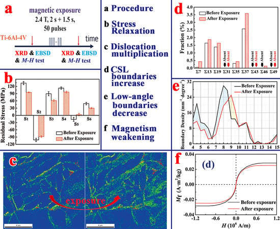
In this work, the influences of a magnetic field of 2.4 T on the macro residual stress and the status of structural defects, including grain boundaries, dislocations and the Fe-rich clusters of Ti-6Al-4V were investigated by X-ray Diffraction (XRD), Electron Backscatter Diffraction (EBSD) and magnetic measurement. The XRD test results show that the applied magnetic field can cause the relaxation and homogenization of macro residual stress. The maps of Kernel Average Misorientation (KAM) values obtained by EBSD tests present a significant dislocation multiplication caused by a magnetic field, and the rise of dislocation density was estimated to be about 32% by XRD tests. The EBSD test results also show an increase in the fraction of Coincidence Site Lattice (CSL) grain boundaries and a decrease in the fraction of low-angle grain boundaries. The results of magnetic measurement show that Ti-6Al-4V has mixed magnetism consisting of paramagnetism and weak ferromagnetism, and that the ferromagnetic saturation magnetization decreased after exposing the alloy to the magnetic field, which suggests the dissolution of the Fe-rich clusters in the alloy. These magnetically-induced changes are related to magnetoplastic effects, a kind of phenomena on which there have been some research, and the possible mechanism of them is discussed in this paper.

1. Introduction

Ti-6Al-4V is the most widely used titanium alloy in aerospace, biomedicine and the petrochemical industry because of its excellent performance, such as high specific strength, fine corrosion resistance, outstanding tissue compatibility and good weldability [1,2,3,4], and various advanced technologies to further enhance its performances have attracted increasing attention [5,6,7]. Magnetoplastic effects first reported in 1987 [8] are a kind of phenomena that can occur in various materials, including metals [9,10,11,12,13,14], semiconductors [9,10,15,16], ionic crystals [8,9,10,17,18,19], etc. Initially, magnetoplastic effects refer to the phenomena that the mobility of dislocations in materials and the macro plasticity of materials increase in a magnetic field. But with the development of the relevant research, now various influences of a magnetic field on the mechanical properties and the status of the structural defects of materials are all usually referred to as magnetoplastic effects [9,20]. As a result of the changes that take place under the magnetic field, besides the simultaneous effects, there are also residual effects which will remain after switching off the field [9,18,19,21]. This is a potential method worth exploring to improve the service behavior of Ti-6Al-4V using magnetic field.

Residual stress and the status of structural defects are important factors determining the service performance of alloys. In addition, Ti-6Al-4V is a typical difficult-to-machine material, therefore, how to reduce the residual stress caused by machining effectively to ensure its dimensional stability in service is a crucial problem. Hence this work aims at investigating the influences of a magnetic field on the macro residual stress and the status of the structural defects of Ti-6Al-4V.

2. Materials and Methods

The alloy Ti-6Al-4V selected in the experiments (composition (wt %): Al~6.1, V~3.8, Fe~0.26, O~0.011, C~0.012, N~0.005 and H~0.001) was kept at 750 °C for 1 h and cooled in air beforehand, and the alloy is formed by an $\mathsf{\alpha }$ phase (hcp) and a $\mathsf{\beta }$ phase (bcc).

The Scanning Electron Microscope (SEM) LYRA3 was employed to observe the microstructure of the alloy, and the metallographic specimen was etched with 4 vol % HF + 10 vol % HNO₃ + 86 vol % H₂O for 5 s. The Energy Dispersive X-ray (EDX) spectrometer equipped in the SEM was employed for the chemical composition analysis of the phases. In addition, the Time-of-Flight Secondary Ion Mass Spectrometer (TOF-SIMS) was used to analyze the distribution of the elements.

The residual stress tests were carried out on six specimens with a size of 40 mm × 25 mm × 25 mm, using the X-ray stress meter μ-X360s, whose collimator diameter is 1 mm. The anode target of the stress meter was vanadium, and thus the wavelength of the X-ray was 2.505 $Å$. The test region of each specimen is at the center of a 40 mm × 25 mm side face that was mechanically polished and electropolished, and the measured variable was the normal stress along the direction of the long side. Then the specimens were exposed to a rectangle-pulsed magnetic field of 2.4 T for 50 pulses, of which the pulse width was 2 s and the intermittent time was 1.5 s. Then the residual stress tests were conducted again at the same positions as before the magnetic exposure.

Dislocations and grain boundaries are typical linear and planar defects, respectively. In order to analyze the status of the dislocations and grain boundaries in Ti-6Al-4V before and after magnetic exposure, we cut the alloy into a specimen with a size of 15 mm × 10 mm × 5 mm, and polished a 15 mm × 10 mm face of it mechanically and electrically as the test surface. Then we scanned the same region with a size of 12 μm × 12 μm on the test surface before and after exposing the specimen to the aforementioned magnetic field, using the EBSD accessory of the Auger electron spectrometer PHI710. The scanned points formed a hexagonal array with a spacing of 0.07 μm. In order to evaluate the change of dislocation density caused by magnetic exposure quantitatively, we did XRD tests on the test surface using X-ray diffractometer D/Max-2500H with a copper anode (whose characteristic X-ray wavelength is 1.542 $Å$) before and after exposure, and analyzed the data with the Williamson–Hall method. The scanning angle range of the XRD tests was $2\theta =30°~90°$, the scanning speed was 2°/min, and the rotation axis was parallel to the short side of the test surface. The length of the line-shape X-ray source of D/Max-2500H is 10 mm, the goniometer circle radius is 185 mm, and the size of the incident slit is 1°, therefore the radiated area varied in the range (4.57~12.48) mm × 10 mm during scanning.

The magnetically stimulated transformation of point defects in semiconductors [16] and ionic crystals [19,21] have been reported. But the similar studies on alloys are rarely seen. Fe is the dominant impurity element in Ti-6Al-4V, and theoretically, if there exist Fe-rich clusters in the alloy, their status would influence the magnetization performance of the alloy. Therefore, we tried to verify the presence of the Fe-rich clusters and investigate the effect of a magnetic field on their status by testing the magnetization performance of the alloy. The alloy was made into three specimens with a size of 2 mm × 2 mm × 1 mm, and the magnetization curves ($M$-$H$ curves) of them were measured by a Superconducting-Quantum-Interference-Device Vibrating Sample Magnetometer (SQUID-VSM) at 300 K with an applied magnetic field intensity varying from 15,000 Oe (1.194 × 10⁶ A/m) to −15,000 Oe and back to 15,000 Oe. Then the specimens were exposed to the aforementioned pulsed magnetic field for 50 pulses, and then the magnetization curves of the specimens were measured again.

3. Results and Discussion

3.1. Microstructure and Element Distribution of the Alloy

The SEM micrographs of the alloy are shown in Figure 1a,b, from which we can see that the lamellar $\mathsf{\beta }$ phase distributes among the $\mathsf{\alpha }$ phase. The chemical compositions of the $\mathsf{\alpha }$ phase and the $\mathsf{\beta }$ phase were measured with EDX. The composition measurement positions 1 and 2 are marked in Figure 1b, and the results are shown in Figure 1c,d. It can be seen that the content of Al in the $\mathsf{\alpha }$ phase is higher than that in the $\mathsf{\beta }$ phase, while the content of V in the $\mathsf{\beta }$ phase is higher than that in the $\mathsf{\alpha }$ phase. It should be noted that EDX is only a semi-quantitative test technique which is not competent for the detection of the elements with a low mass fraction.

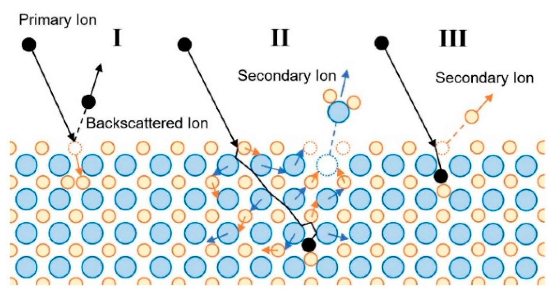
The Time-of-Flight Secondary Ion Mass Spectrometer (TOF-SIMS) is an element detection technique with higher sensitivity and higher space resolution (<40 nm) than EDX. As is shown in Figure 2, when the primary ions (Xe⁺ was used in this work) strike the surface of the solid, the backscattered ions and the secondary ions including the simple ions and charged structure fragments will be produced. The types of the ions can be identified according to their mass–charge ratios. Therefore TOF-SIMS can be used to investigate the element distribution qualitatively and provide some information about the substance structure.

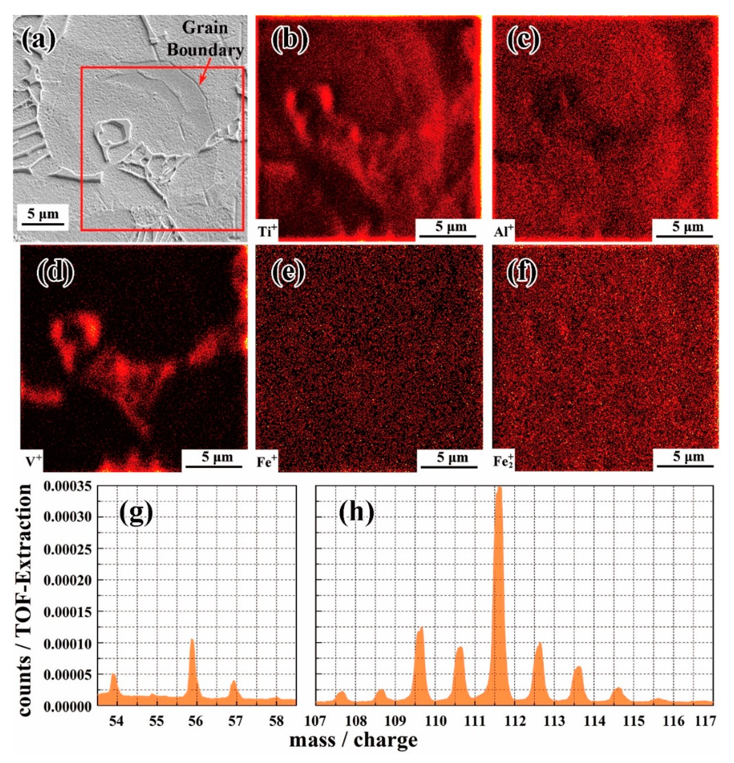
Figure 3b–f show the secondary-ion images of the region marked by the red box in Figure 3a, which are obtained by detecting Ti⁺, Al⁺, V⁺, Fe⁺ and Fe₂⁺ with TOF-SIMS. In a secondary-ion image, the brightness is proportional to the production of the secondary ions, which is mainly determined by the element content, and also affected by the topography and properties of the substrate. It can be seen that the content differences of Al and V between the $\mathsf{\alpha }$ phase and $\mathsf{\beta }$ phase, which are shown in Figure 3c,d, are consistent with the EDX test results. As is shown in Figure 3e,f, the distribution of Fe is basically uniform, and no obvious enrichment of Fe at the grain boundaries was detected.

What is noteworthy is that a lot of di-iron cations Fe₂⁺ were detected in the TOF-SIMS test, and the count of them exceeds that of Fe⁺ (the mass spectrum peaks of Fe⁺ and Fe₂⁺ are shown in Figure 3g,h, respectively). Therefore it is logical to suppose that there exist a lot of Fe-rich clusters in the alloy, from the fragmentation of which a lot of Fe₂⁺ can be produced.

3.2. Effects of Magnetic Field on Residual Stress

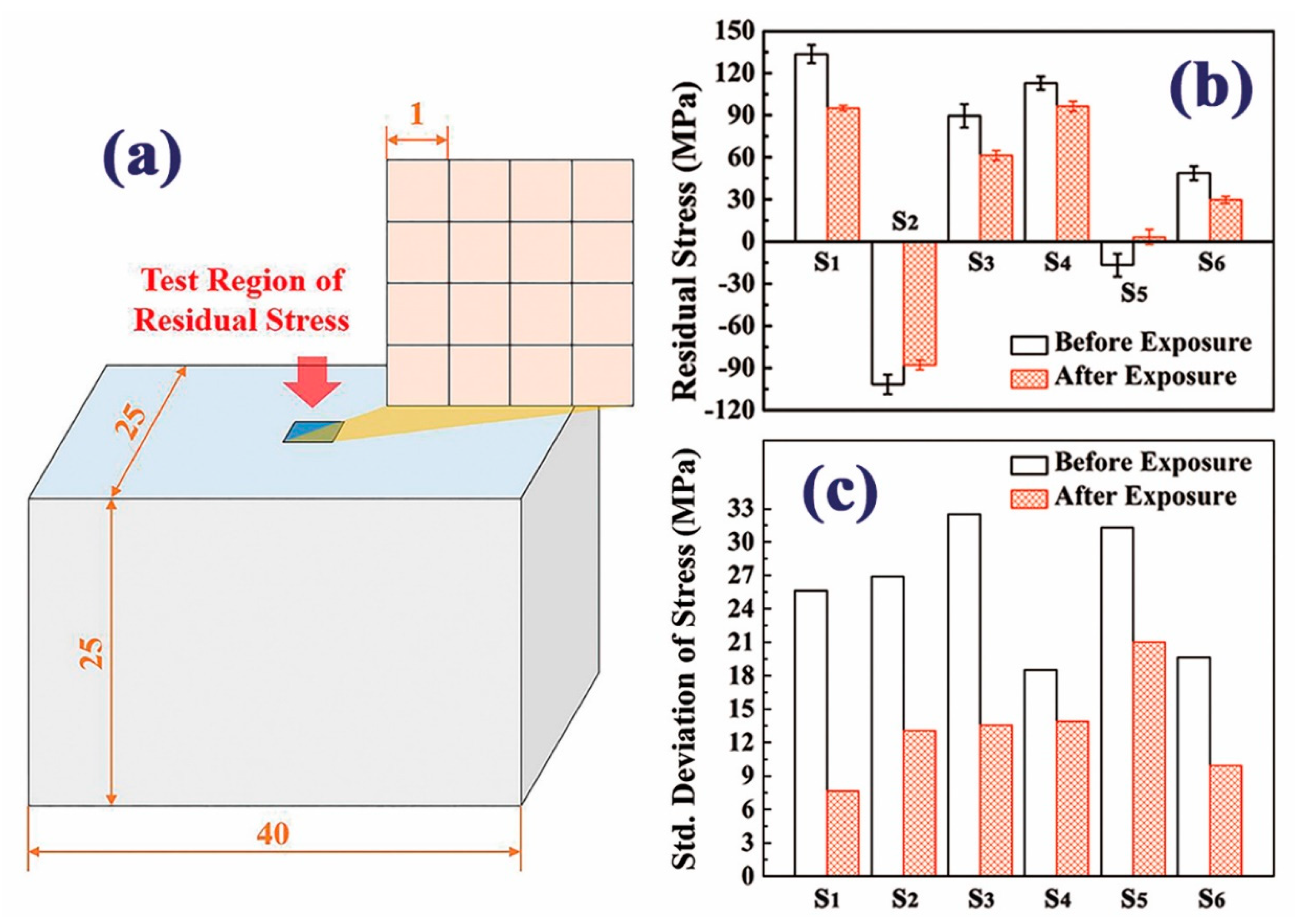
In order to reduce the test error of the residual stress, we measured the residual stress in the test region of each specimen for 16 times. As is shown in Figure 4a, the test region is a square area with a size of 4 mm × 4 mm at the center of a 40 mm × 25 mm side face of the specimen, and the 16 test points formed a matrix with a spacing of about 1 mm. The average of the 16 test values was taken as the residual stress of the test region, and those of the six specimens before and after magnetic exposure are shown in Figure 4b.

It can be seen that the stress values of the six specimens’ test regions after magnetic exposure were reduced to a different extent compared with those before exposure, and this indicates that exposing Ti-6Al-4V to the magnetic field can bring about a macro residual stress relaxation of the alloy.

Figure 4c shows the standard deviations of the stress test values of each specimen’s test region before and after the magnetic field, which can reflect the inhomogeneity of the residual stress in the test region, namely the level of the mm-scale stress. We can see that the residual stress deviations after magnetic exposure significantly decreased compared with those before exposure. This indicates that the magnetic field can prompt the homogenization of the residual stress of Ti-6Al-4V.

3.3. Effects of Magnetic Field on Status of Dislocations

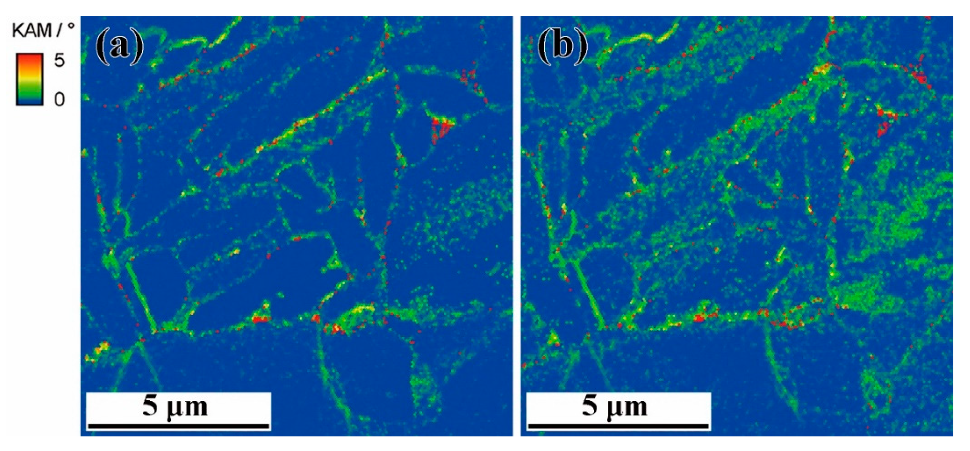
The lattice orientation at each position can be measured by the EBSD test. Additionally, the KAM (Kernel Average Misorientation) value, which is defined as the average of the misorientations between one scanned point and the six adjacent scanned points, is a common scalar parameter used to be an approximate characterization of the dislocation density in EBSD analysis [22,23]. Actually, it has been proven that KAM is proportional to the geometrically necessary dislocation density, and KAM is invariant under in-plane rotation [24], which means that a minor change of the specimen displacement direction of the EBSD scan hardly influences the KAM values. Therefore, we did EBSD tests in the same region on a Ti-6Al-4V specimen before and after exposing it to the magnetic field, and obtained the KAM maps, which are shown in Figure 5.

Comparing Figure 5b with Figure 5a, we can see a significant rise in KAM, and this indicates the multiplication of dislocations that took place under the action of the magnetic field.

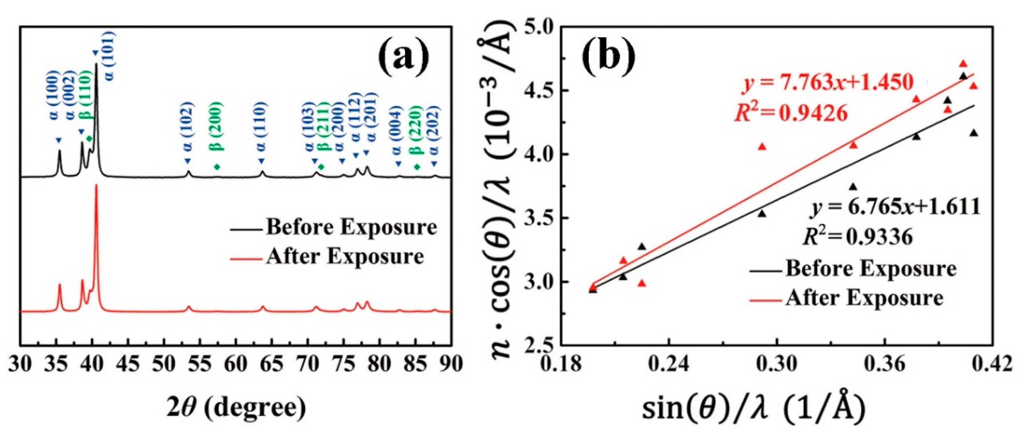
Besides the EBSD tests, in order to give a quantitative evaluation of the influence of magnetic exposure on the dislocation density, we did XRD tests on the test surface of the specimen before and after magnetic exposure. The XRD patterns are shown in Figure 6a. The diffraction peaks of the $\mathsf{\alpha }$ phase are clear, while most of the diffraction peaks of the $\mathsf{\beta }$ phase are too weak to identify. On the basis of the XRD test data, we estimated the amount of the rise in dislocation density of the $\mathsf{\alpha }$ phase according to the Williamson–Hall formulation [25,26,27] $n\cos \theta /\lambda =2/D+4e\sin \theta /\lambda$, where $n$ is the full width at half maximum (FWHM) of the diffraction peak, $\theta$ is the diffraction angle of the peak, $\lambda$ is the X-ray wavelength equaling 1.542 $Å$, $D$ is the characteristic grain size and $e$ is the lattice strain which has the relationship [28] $\rho \approx 16e^2/{\mathit{b}}^2$ with the dislocation density $\rho$ and the Burgers vector $\mathit{b}$ ($b=2.93 Å$ for the $\mathsf{\alpha }$ phase of Ti-6Al-4V). In order to obtain the FWHM and diffraction angle of every peak, we firstly got the physical shapes of the peaks through multiple peak fitting and the removal of instrument peak shapes, and then obtained these two parameters from the physical peak shapes. The nine strongest $\mathsf{\alpha }$ phase peaks were selected to estimate the dislocation density in the $\mathsf{\alpha }$ phase of the specimen before and after magnetic exposure, and the linear fitting results of $n\cos \theta /\lambda$ and $\sin \theta /\lambda$ are shown in Figure 6b.

The slopes of the fitting lines of $n\cos \theta /\lambda$ and $\sin \theta /\lambda$ before and after magnetic exposure are $6.765\times {10}^{-3}$ and $7.763\times {10}^{-3}$ respectively, and the coefficients of determination $R^2$ of the fitting results are 0.9336 and 0.9426. Thus the dislocation density in the $\mathsf{\alpha }$ phase of the specimen before and after magnetic exposure can be estimated to be 533 μm⁻² and 702 μm⁻², the latter of which is larger than the former by roughly 32%.

3.4. Effects of Magnetic Field on Status of Grain Boundaries

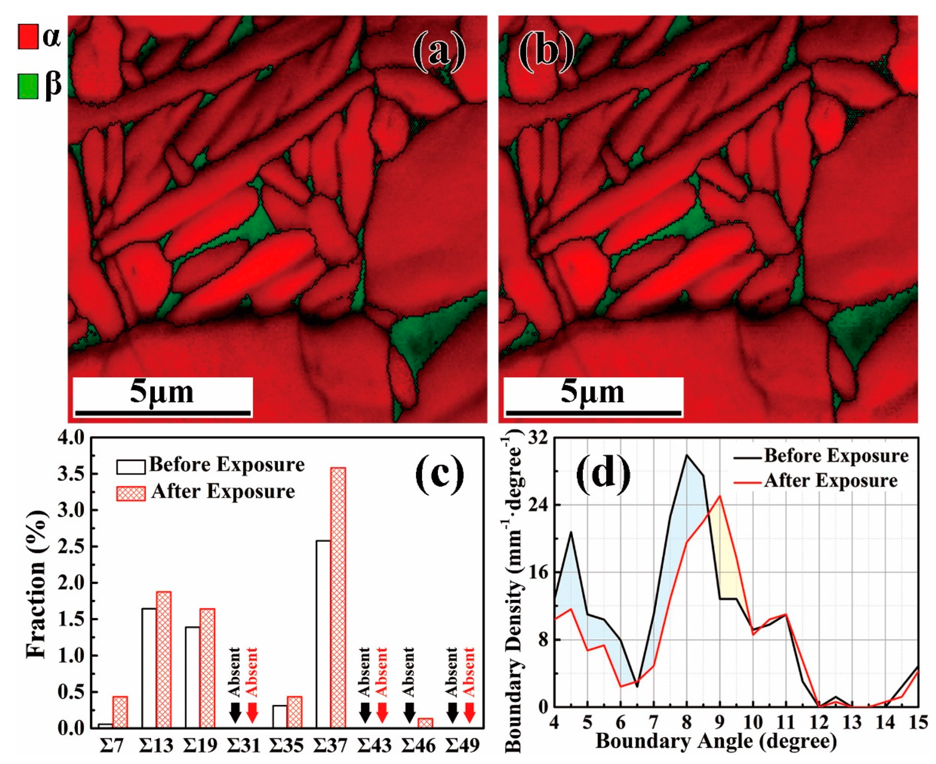
The phases and grain boundaries can be identified according to the EBSD test data, and the maps of the phases and grain boundaries before and after magnetic exposure are shown in Figure 7a,b. It can be seen that the $\mathsf{\alpha }$ phase is the dominant phase of the alloy, whose fractions before and after magnetic exposure were calculated to be 94.3% and 94.1%, respectively (The analysis error being considered, this difference cannot be regarded as significant). We made a statistical analysis of the grain boundaries between the $\mathsf{\alpha }$ phase grains.

Coincidence Site Lattice (CSL) grain boundaries are a special kind of grain boundaries with a relatively lower grain boundary energy, and are therefore more stable than the ordinary grain boundaries. For the $\mathsf{\alpha }$ phase of Ti-6Al-4V, there are nine main kinds of CSL grain boundaries in theory, namely Σ7 (meaning there is one coincidence site in per 7 lattice sites), Σ13, Σ19, Σ31, Σ35, Σ37, Σ43, Σ46, and Σ49. The proportions of these CSL grain boundaries in the total grain boundaries before and after magnetic exposure are shown in Figure 7c. We can see that each kind of CSL grain boundaries significantly increased after magnetic exposure, and the total proportion of the existing CSL grain boundaries increased from about 5.98% to about 8.10%. Especially, the proportion of Σ37 grain boundaries, which accounts for the highest proportion among the CSL grain boundaries whether before or after magnetic exposure, increased from about 2.58% to about 3.58% through magnetic exposure.

Meanwhile, we calculated the densities of low-angle grain boundaries before and after magnetic exposure, and the results are shown in Figure 7d. As is shown, after exposure, the amount of low-angle grain boundaries significantly decreased, but there is an increase in the amount of the grain boundaries with an angle of about 8.7~10°. Actually, the angle of the Σ37 grain boundaries of the $\mathsf{\alpha }$ phase is around 9.4°, so the increase of the grain boundaries in the range of 8.7~10° is consistent with the increase of the Σ37 grain boundaries.

The changes of the amounts of the CSL grain boundaries and the low-angle grain boundaries caused by the magnetic treatment indicate that the magnetic field can stimulate the adjustment of the atomic positions in the vicinity of the grain boundaries, which can result in some grain boundaries satisfying the condition of the coincidence site lattice and the disappearance of some low-angle grain boundaries, so that the lattice can reach a more stable state.

3.5. Effects of Magnetic Field on Status of Fe-Rich Clusters

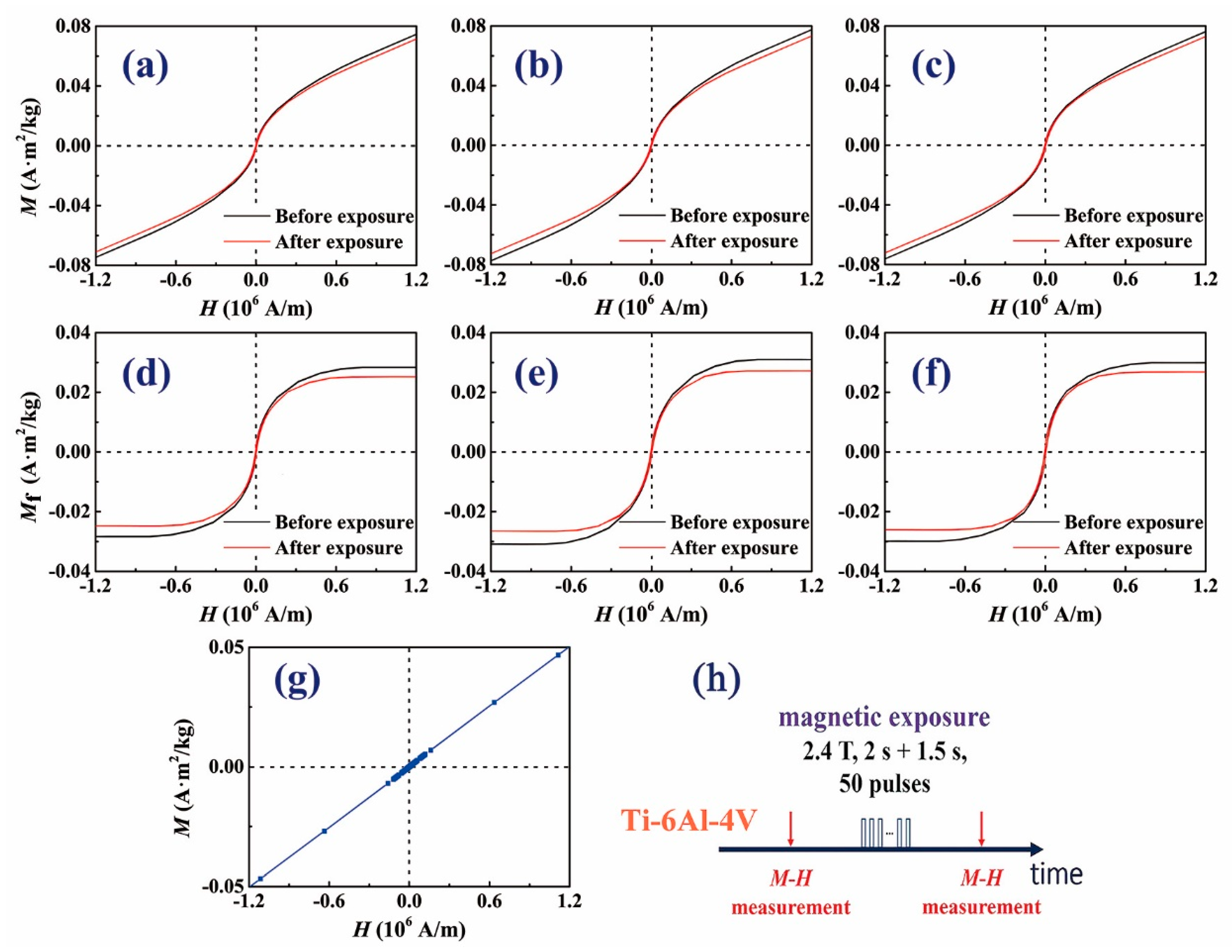
According to the fact that a lot of di-iron cations Fe₂⁺ were detected in the SIMS test (Figure 3h), it has been logically supposed that there exist a lot of Fe-rich clusters in Ti-6Al-4V. Theoretically, the presence of the Fe-rich cluster may bring about a slight ferromagnetism of the alloy. In order to further verify the presence of the Fe-rich clusters and to investigate the influence of the magnetic field on their status, we conducted magnetic measurements on Ti-6Al-4V, and the results are shown in Figure 8a–c.

It can be seen that the magnetism of Ti-6Al-4V is not pure paramagnetism, but a mixed magnetism containing weak ferromagnetism. The sections of each magnetization curve at a high magnetic field intensity ($\left|H\right|>7\times {10}^5$ A/m) almost become straight lines, the slopes of which are the mass susceptibility ${\chi }_{\mathrm{p}}$ of the paramagnetic part of the magnetization. Therefore the paramagnetic susceptibilities ${\chi }_{\mathrm{p}}$ of the three specimens before exposure are calculated to be 3.859 × 10⁻⁸ m³/kg, 3.883 × 10⁻⁸ m³/kg and 3.859 × 10⁻⁸ m³/kg by linear fitting (The sections of $H>7\times {10}^5$ A/m and $H<-7\times {10}^5$ A/m are fitted separately, and the average of the two slopes is taken as the final result), while those after exposure are respectively 3.863 × 10⁻⁸ m³/kg, 3.847 × 10⁻⁸ m³/kg and 3.849 × 10⁻⁸ m³/kg. These results show that the magnetic exposure has no significant effect on the paramagnetic susceptibility of the alloy.

The logical explanation of the weak ferromagnetism of the alloy is that there exist Fe-rich clusters with spontaneous magnetization, and the directions of their magnetic moments will tend to be consistent under the action of an applied magnetic field. As a contrast, the magnetization curve of a high-purity titanium specimen with a purity of over 99.995 wt % was measured, and the result is shown in Figure 8g. As is shown, the magnetism of high-purity titanium is almost pure paramagnetism with a mass susceptibility of 4.178 × 10⁻⁸ m³/kg, which suggests that the weak ferromagnetism of Ti-6Al-4V is due to the Fe composition.

The ferromagnetic part of the magnetization can be calculated according to the formula $M_{\mathrm{f}}=M-{\chi }_{\mathrm{p}}H$, and the $M_{\mathrm{f}}$-$H$ curves of the specimens are shown in Figure 8d–f. It can be seen that the ferromagnetic saturation magnetizations of the specimens before exposure are 2.833 × 10⁻² A·m²/kg, 3.096 × 10⁻² A·m²/kg and 2.989 × 10⁻² A·m²/kg, respectively, while those after exposure are 2.516 × 10⁻² A·m²/kg, 2.717 × 10⁻² A·m²/kg and 2.678 × 10⁻² A·m²/kg, which are, respectively, 88.81%, 87.76% and 89.60% of those before exposure. Thus the ferromagnetism of the specimens were significantly weakened by magnetic exposure.

The decrease in the ferromagnetic saturation magnetization caused by magnetic exposure suggests that the dissolution of the Fe-rich clusters can take place during magnetic exposure, which will result in the reduction of the amount of agglomerating iron atoms, and thereby result in the reduction of the spontaneous magnetic moment of each cluster.

3.6. Possible Mechanism of the Magnetically Stimulated Variations

The relaxation and homogenization of the residual stress are essentially consistent with the multiplication of the dislocations, which can be regarded as a special slip creepage stimulated by the magnetic field. Additionally, all of the changes of the structural defects reported in this paper are atom-migration-related processes, because the slippage and multiplication of dislocations, the change of grain boundary structure, and the dissolution of clusters are all finished through the atomic migration among adjacent sites. Therefore, these magnetically stimulated changes indicate that the atomic mobility is enhanced under the action of a magnetic field, and this is the essential feature of magnetoplastic effects.

It should be pointed out that the magnetoplastic effects are difficult to be explained in terms of energy, especially for the non-ferromagnetic materials, because the energy induced by a magnetic field with an intensity of several Teslas is ignorable, compared with the thermal energy at room temperature (${\mu }_{\mathrm{B}}B={10}^{-4}~{10}^{-3}kT$, where ${\mu }_{\mathrm{B}}$ is the Bohr magneton, B is the magnetic flux density, $k$ is the Boltzmann constant, and $T$ is the thermodynamic temperature). Thus the magnetic field must affect the kinetic nature of the atom-migration-related processes.

On the basis of the features of the magnetoplastic effects revealed in the relevant research, especially some features related to electron spin resonance found by experiments [9,19,29], it is generally accepted that the dominant mechanism of magnetoplastic effects is the spin-dependent variations of electron pairs [17,18,19,20,21,29,30,31]. For example, as to the mechanism of the magnetically stimulated depinning of dislocations, Morgunov [21] and Buchachenko [21,29] gave an appropriate explanation for ionic crystals: Once one of a pair of electrons of an anion in the dislocation core transfers onto the positively-charged obstacle due to thermal excitation, the Coulomb interaction pinning the dislocation at the obstacle is “switched off”, and the electron pair is in singlet state (meaning the total spin of the pair is 0) because of the Spin Selection Rule (An electron does not change its spin in transition); the magnetic field stimulates the intersystem crossing from singlet state to triplet state (meaning the total spin of the pair is 1), so that the system with switched-off Coulomb potential has a longer lifetime (because the transition from triplet state to ground state is spin-forbidden due to the Spin Selection Rule), which brings about a higher depinning rate. In the previous research weapplied the similar theory to covalent crystals and the atom-migration-related processes besides dislocation depinning [16], since a covalent electron pair can also be thermally excited into the excited state with a lower binding energy than the ground state, and the atomic migration will be promoted if the lifetime of the excited state is extended.

It is obvious that the mechanism described in the preceding paragraph is based upon the discussion of electrons using a localized model. However, because of the particularity of metallic bonds, they are usually explained using delocalized models, such as the Drude–Lorents theory, which describes metal bonding as the Coulomb interaction between metal cations and free electrons. Thus there is some difficulty in applying the above-mentioned mechanism directly to metals and alloys. But it is appropriate to regard the defect electronic energy levels as localized. In addition, the metallic bond can also be analyzed using localized models, such as the covalent theory of metals [32], which attributes metal bonding partially to the covalent bond. This make it possible to apply the magnetically-induced-intersystem-crossing mechanism to the magnetoplastic effects of metals and alloys. Briefly put, the excited state lifetimes of bonding electron pairs become longer because of the intersystem crossing caused by the magnetic field, leading to the atom-migration-related processes being promoted. Of course, this needs further argumentation.

The mechanism of magnetically introduced intersystem crossing can be explained as follows. The spin functions of the singlet state $S$ and the triplet state $T_0$ with a spin projection of 0 are respectively $S=\left(\alpha \beta -\beta \alpha \right)/\sqrt{2}$ and $T_0=\left(\alpha \beta -\beta \alpha \right)/\sqrt{2}$, where $\alpha$ and $\beta$ are the wave functions of the single-electron spin eigenstates with upward and downward spin, respectively. Additionally, the spin-related part of the Hamiltonian is $\hat{H}={\mu }_{\mathrm{B}}B\left(g_1{\hat{S}}_1+g_2{\hat{S}}_2\right)/\hslash$, where ${\hat{S}}_1$ and ${\hat{S}}_2$ are the spins of the partners, $g_1$ and $g_2$ are their Lande factors, and $\hslash$ is the reduced Planck constant. We can derive

$$\left[\begin{array}{cc}\langle S\left|\hat{H}\right|S\rangle & \langle S\left|\hat{H}\right|T_0\rangle \\ \langle T_0\left|\hat{H}\right|S\rangle & \langle T_0\left|\hat{H}\right|T_0\rangle \end{array}\right] = \frac{1}{2}\left(g_1-g_2\right){\mu }_{\mathrm{B}}B\left[\begin{array}{cc}0& 1\\ 1& 0\end{array}\right] = \frac{1}{2}\mathsf{\Delta }g{\mu }_{\mathrm{B}}B\left[\begin{array}{cc}0& 1\\ 1& 0\end{array}\right].$$

According to the Schrodinger equation $\mathrm{i}\hslash \partial \phi /\partial t=\hat{H}\phi$, it is obtained that the spin wave function of an electron pair is $\phi \left(t\right)=\cos \left(\mathsf{\Delta }g{\mu }_{\mathrm{B}}Bt/2\hslash \right)S-\mathrm{i}\sin \left(\mathsf{\Delta }g{\mu }_{\mathrm{B}}Bt/2\hslash \right)T_0$. Therefore, the probabilities of the electron pair being in $S$ state and $T_0$ state are, respectively, $P\left(S\right)={\cos }^2\left(\mathsf{\Delta }g{\mu }_{\mathrm{B}}Bt/2\hslash \right)=\left[1+\cos \left(\mathsf{\Delta }g{\mu }_{\mathrm{B}}Bt/\hslash \right)\right]/2$ and $P\left(T_0\right)={\sin }^2\left(\mathsf{\Delta }g{\mu }_{\mathrm{B}}Bt/2\hslash \right)=\left[1-\cos \left(\mathsf{\Delta }g{\mu }_{\mathrm{B}}Bt/\hslash \right)\right]/2$, which means that the magnetic field can cause the intersystem crossing between $S$ and $T_0$ with a frequency of ${\mu }_{\mathrm{B}}\mathsf{\Delta }gB/h$, where $h$ is the Planck constant.

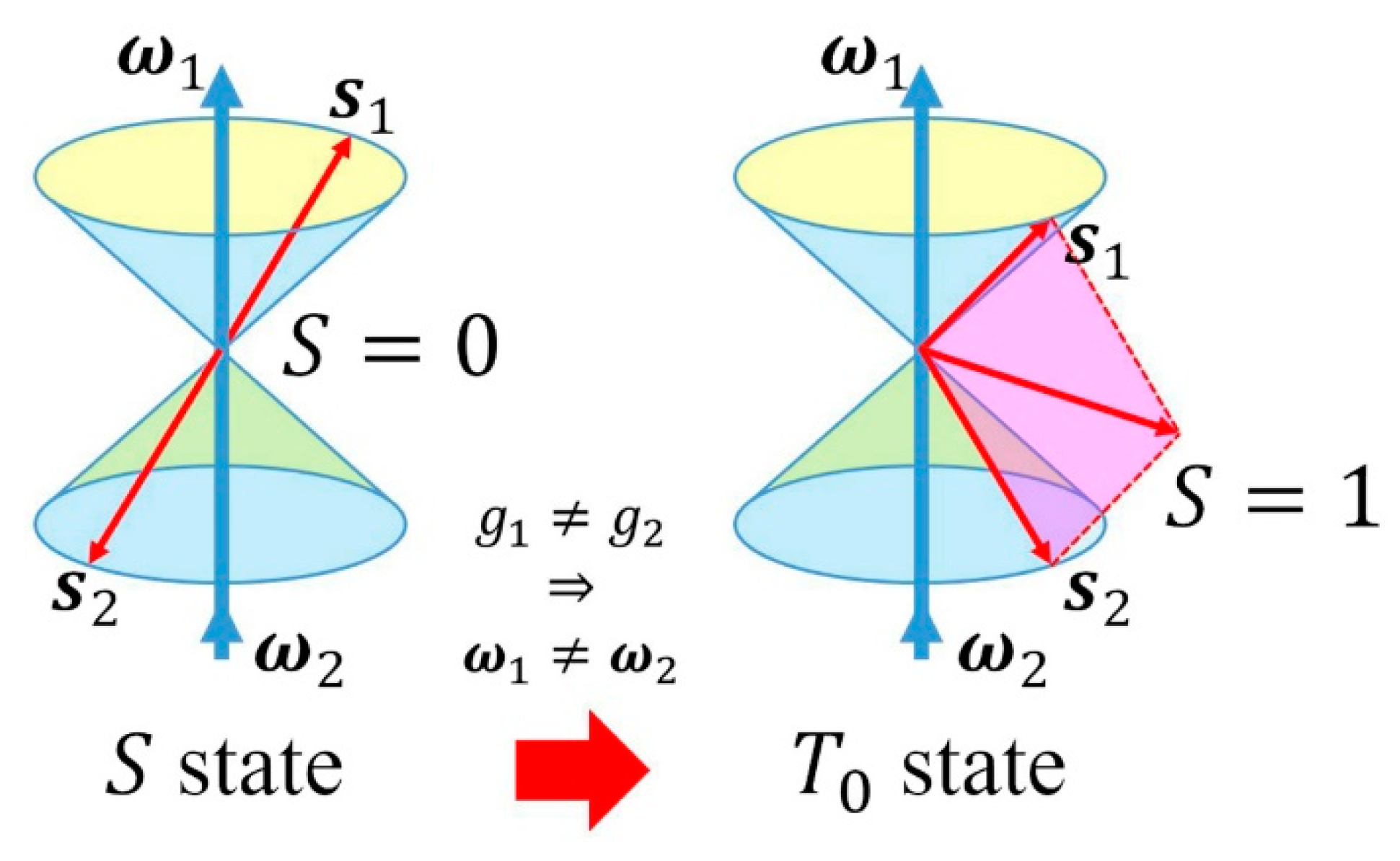
There is a visualized understanding for this mechanism, which is widely referred to [20,33]. The visualized diagrams of singlet state $S$ and triplet state $T_0$ are shown in Figure 9. A magnetic field will cause the Larmor precession of an electron with a frequency of $g{\mu }_{\mathrm{B}}B/h$ which is called the Larmor frequency. Because of the difference between the Lande factors of the two electrons, their Larmor frequencies have a difference of ${\mu }_{\mathrm{B}}\mathsf{\Delta }gB/h$, and this is just the frequency of the intersystem crossing between the $S$ state and the $T_0$ state. This mechanism is usually referred to as the $\mathsf{\Delta }g$ mechanism.

4. Conclusions

A magnetic field with a magnetic flux density of 2.4 T can stimulate the relaxation and homogenization of the residual stress, the multiplication of dislocations, the increase in the amount of CSL boundaries and the decrease in the amount of low-angle boundaries of Ti-6Al-4V. In addition, the weakening of the slight ferromagnetism of Ti-6Al-4V caused by magnetic exposure suggests that the magnetic field can prompt the dissolution of the Fe-rich clusters in the alloy. These results suggest the potential of magnetic treatment in the processing of Ti-6Al-4V.

The magnetically stimulated changes of the macro residual stress and the status of structural defects indicate that the atomic mobility is enhanced by the magnetic field, which is the essential feature of magnetoplastic effects. Based on the point that metal bonding can be analyzed using the localized model, the possible mechanism of the magnetoplastic effects of Ti-6Al-4V is put forward as follows. The magnetic field can cause the intersystem crossing of the bonding electron pairs that have been thermally excited, transforming them from singlet state to triplet state, and thereby making the excited state lifetime longer, and as a result, the atomic mobility is enhanced and the atom-migration-related processes are prompted. This mechanism still needs further argumentation.

References

- Manikandan, N.; Arulkirubakaran, D.; Palanisamy, D.; Raju, R. Influence of wire-EDM textured conventional tungsten carbide inserts in machining of aerospace materials (Ti–6Al–4V alloy). Mater. Manuf. Process. 2018, 34, 103–111. [Google Scholar] [CrossRef]
- Wang, K. The use of titanium for medical applications in the USA. Mater. Sci. Eng. A 1996, 213, 134–137. [Google Scholar] [CrossRef]
- Venkatesh, B.D.; Chen, D.L.; Bhole, S.D. Effect of heat treatment on mechanical properties of Ti–6Al–4V ELI alloy. Mater. Sci. Eng. A 2009, 506, 117–124. [Google Scholar] [CrossRef]
- Sharifi, F.; Abouei, V.; Alizadeh, A.; Shajari, Y.; Porhonar, M.; Ghanbari, M.; Ravari, B.K. The effect of different heat treatment cycle on hot corrosion and oxidation behavior of Ti-6Al-4V. Mater. Res. Express 2019, 6, 116599. [Google Scholar] [CrossRef]
- Kobryn, P.A.; Semiatin, S.L. The laser additive manufacture of Ti-6Al-4V. JOM 2001, 53, 40–42. [Google Scholar] [CrossRef]
- Thijs, L.; Verhaeghe, F.; Craeghs, T.; Van Humbeeck, J.; Kruth, J.P. A study of the micro structural evolution during selective laser melting of Ti-6Al-4V. Acta Mater. 2010, 58, 3303–3312. [Google Scholar] [CrossRef]
- Ya, B.; Zhou, B.; Yang, H.; Huang, B.; Jia, F.; Zhang, X. Microstructure and mechanical properties of in situ casting TiC/Ti6Al4V composites through adding multi-walled carbon nanotubes. J. Alloys Compd. 2015, 637, 456–460. [Google Scholar] [CrossRef]
- Al’shits, V.I.; Darinskaya, E.V.; Perekalina, T.M.; Urusovskaya, A.A. Motion of dislocations in NaCl crystals under the action of a static magnetic field. Sov. Phys. Solid State 1987, 29, 265–267. [Google Scholar]
- Golovin, Y.I. Magnetoplastic effects in solids. Phys. Solid State 2004, 46, 789–824. [Google Scholar] [CrossRef]
- Alshits, V.I.; Darinskaya, E.V.; Koldaeva, M.V.; Petrzhik, E.A. Magnetoplastic effect: Basic properties and physical mechanisms. Crystallogr. Rep. 2003, 48, 768–795. [Google Scholar] [CrossRef]
- Su, Y.Y.; Hochman, R.F.; Schaffer, J.P. A positron annihilation spectroscopy investigation of magnetically induced changes in defect structures. J. Phys. Condens. Matter 1990, 2, 3629–3642. [Google Scholar] [CrossRef]
- Li, C.; He, S.; Fan, Y.; Engelhardt, H.; Jia, S.; Xuan, W.; Li, X.; Zhong, Y.; Ren, Z. Enhanced diffusivity in Ni-Al system by alternating magnetic field. Appl. Phys. Lett. 2017, 110, 074102. [Google Scholar] [CrossRef]
- Yuan, Z.; Ren, Z.; Li, C.; Xiao, Q.; Wang, Q.; Dai, Y.; Wang, H. Effect of high magnetic field on diffusion behavior of aluminum in Ni-Al alloy. Mater. Lett. 2013, 108, 340–342. [Google Scholar] [CrossRef]
- Wang, H.M.; Li, P.S.; Zheng, R.; Li, G.R.; Yuan, X.T. Mechanism of high pulsed magnetic field treatment of the plasticity of aluminum matrix composites. Acta Phys. Sin. 2015, 64, 087104. [Google Scholar]
- Orlov, A.M.; Skvortsov, A.A.; Gonchar, L.I. Magnetically simulated variation of dislocation mobility in plastically deformed n-silicon. Phys. Solid State 2001, 43, 1252–1256. [Google Scholar] [CrossRef]
- Zhang, X.; Cai, Z.P. Effect of magnetic field on the nanohardness of monocrystalline silicon and its mechanism. JETP Lett. 2018, 108, 23–29. [Google Scholar] [CrossRef]
- Alshits, V.I.; Darinskaya, E.V.; Kazakova, O.L. Magnetoplastic effect in irradiated NaCl and LiF crystals. J. Exp. Theor. Phys. 1997, 84, 338–344. [Google Scholar] [CrossRef]
- Golovin, Y.I.; Morgunov, R.B.; Lopatin, D.V.; Baskakov, A.A.; Evgen’ev, Y.E. Reversible and irreversible magnetic-field-induced changes in the plastic properties of NaCl crystals. Phys. Solid State 1998, 40, 1870–1872. [Google Scholar] [CrossRef]
- Golovin, Y.I.; Morgunov, R.B. Effect of a weak magnetic field on the state of structural defects and the plasticity of ionic crystals. J. Exp. Theor. Phys. 1999, 88, 332–341. [Google Scholar] [CrossRef]
- Golovin, Y.I. Magnetoplastic effects in crystals in the context of spin-dependent chemical kinetics. Crystallogr. Rep. 2004, 49, 668–675. [Google Scholar] [CrossRef]
- Morgunov, R.B.; Buchachenko, A.L. Magnetoplasticity and magnetic memory in diamagnetic solids. J. Exp. Theor. Phys. 2009, 109, 434–441. [Google Scholar] [CrossRef]
- Kamaya, M.; Wilkinson, A.J.; Titchmarsh, J.M. Measurement of plastic strain of polycrystalline material by electron backscatter diffraction. Nucl. Eng. Des. 2005, 235, 713–725. [Google Scholar] [CrossRef]
- Fujiyama, K.; Mori, K.; Kaneko, D.; Kimachi, H.; Saito, T.; Ishii, R.; Hino, T. Creep damage assessment of 10Cr-1Mo-1W-VNbN steel forging through EBSD observation. Int. J. Press. Vessel. Pip. 2009, 86, 570–577. [Google Scholar] [CrossRef]
- Rui, S.S.; Niu, L.S.; Shi, H.J.; Wei, S.L.; Tasan, C.C. Diffraction-based misorientation mapping: A continuum mechanics description. J. Mech. Phys. Solids 2019, 133, 103709. [Google Scholar] [CrossRef]
- Zak, A.K.; Majid, W.H.A.; Abrishami, M.E.; Yousefi, R. X-ray analysis of ZnO nanoparticles by Williamson-Hall and size-strain plot methods. Solid State Sci. 2011, 13, 251–256. [Google Scholar]
- Mote, V.D.; Purushotham, Y.; Dole, B.N. Williamson-Hall analysis in estimation of lattice strain in nanometer-sized ZnO particles. J. Theor. Appl. Phys. 2012, 6, 6. [Google Scholar] [CrossRef] [Green Version]
- Aly, K.A.; Khalil, N.M.; Algamal, Y.; Saleem, Q.M.A. Lattice strain estimation for CoAl2O4 nano particles using Williamson-Hall analysis. J. Alloys Compd. 2016, 676, 606–612. [Google Scholar] [CrossRef]
- Williamson, G.K.; Smallman, R.E. Dislocation densities in some annealed and cold-worked metals from measurements on the x-ray Debye-Scherrer spectrum. Philos. Mag. 1956, 1, 34–46. [Google Scholar] [CrossRef]
- Buchachenko, A.L. Magnetoplasticity of diamagnetic crystals in microwave fields. J. Exp. Theor. Phys. 2007, 105, 593–598. [Google Scholar] [CrossRef]
- Darinskaya, E.V.; Petrzhik, E.A.; Erofeev, S.A.; Kisel’, V.P. Magnetoplastic effect in InSb. JETP Lett. 1999, 70, 309–313. [Google Scholar] [CrossRef]
- Molotskii, M.; Fleurov, V. Spin effects in plasticity. Phys. Rev. Lett. 1997, 78, 2779–2782. [Google Scholar] [CrossRef]
- Wang, F.E. Bonding Theory for Metals and Alloys; Elsevier: Amsterdam, The Netherlands, 2005; pp. 6–7. [Google Scholar]
- Turro, N.J. Micelles, magnets and molecular mechanisms—Application to cage effects and isotope-separation. Pure Appl. Chem. 1981, 53, 259–286. [Google Scholar] [CrossRef] [Green Version]
Figure 1.
(a,b) The Scanning Electron Microscope (SEM) micrographs of the alloy Ti-6Al-4V, and the Energy Dispersive X-ray (EDX) measurement results of (c) position 1 and (d) position 2 marked in (b).
Figure 2.
The diagram of the production of the backscattered ions (I) and the secondary ions (II and III). The secondary ions include fragment ions (II) and simple ions (III).
Figure 3.
(a) The SEM micrograph of the alloy Ti-6Al-4V, (b–f) the secondary ion images of the region marked in (a), and the mass spectrum peaks (including the isotope peaks) of (g) Fe+ and (h) Fe2+.
Figure 4.
(a) The diagram of the test region of each residual stress specimen; (b) the residual stress values of each specimen’s test region before and after magnetic exposure, where the error bars represent the standard errors which are determined by ; (c) the standard deviations of the stress test values of each specimen’s test region before and after magnetic exposure, which are determined by .
Figure 5.
The Kernel Average Misorientation (KAM) maps of the Ti-6Al-4V specimen (a) before and (b) after magnetic exposure.
Figure 6.
(a) The X-ray diffractometry (XRD) patterns of the Ti-6Al-4V specimen and (b) the linear fitting of the strongest nine -phase peaks before and after magnetic exposure, where is the full width at half maximum (FWHM) ( ) of the physical peak shape and is the X-ray wavelength equaling 1.542 .
Figure 7.
The maps of the phases and grain boundaries of the Ti-6Al-4V specimen (a) before and (b) after magnetic exposure; the statistical charts of (c) Coincidence Site Lattice (CSL) grain boundaries and (d) low-angle grain boundaries before and after magnetic exposure.
Figure 8.
(a–c) The magnetization curves of the Ti-6Al-4V specimens and (d–f) the ferromagnetic components of the magnetization curves before and after magnetic exposure; (g) the magnetization performance of high-purity titanium with a purity of over 99.995 wt %; (h) the operation procedures of Ti-6Al-4V specimens.
Figure 9.
A visualized diagram of the mechanism of magnetically induced intersystem crossing.
© 2020 by the authors. Licensee MDPI, Basel, Switzerland. This article is an open access article distributed under the terms and conditions of the Creative Commons Attribution (CC BY) license (http://creativecommons.org/licenses/by/4.0/).
Share and Cite
MDPI and ACS Style
Zhang, X.; Zhao, Q.; Cai, Z.; Pan, J. Effects of Magnetic Field on the Residual Stress and Structural Defects of Ti-6Al-4V. Metals 2020, 10, 141. https://doi.org/10.3390/met10010141
AMA Style
Zhang X, Zhao Q, Cai Z, Pan J. Effects of Magnetic Field on the Residual Stress and Structural Defects of Ti-6Al-4V. Metals. 2020; 10(1):141. https://doi.org/10.3390/met10010141
Chicago/Turabian StyleZhang, Xu, Qian Zhao, Zhipeng Cai, and Jiluan Pan. 2020. "Effects of Magnetic Field on the Residual Stress and Structural Defects of Ti-6Al-4V" Metals 10, no. 1: 141. https://doi.org/10.3390/met10010141
Note that from the first issue of 2016, this journal uses article numbers instead of page numbers. See further details here.