Dimensional Analysis of Superplastic Processes with the Buckingham Π Theorem

Abstract

This work applies the Buckingham $\Pi$ theorem from dimensional analysis on superplastic processes in order to obtain laws of behaviour in a simple way. For this reason, a mathematical background is developed. The particular behaviour of superplastic materials makes it necessary to adapt the way in which these are treated, modelling them by a viscosity function of the strain-rate. Then, dimensional analysis is applied on a set of free-inflation tests in order to obtain a formula that defines the forming time as single function of geometric and material variables. Dimensional analysis allows us to reduce the number of variables to analyse from six to only three. Finally, two different forming time estimators are compared to measure the accuracy of our method, showing a significant improvement over previous methods.

1. Introduction

Superplastic forming (SPF) is a manufacturing technique that allows us to form complex shape parts in a single operation [1]. It is widely used in the automotive [2] and the aerospace [3,4] industry, predominantly in applications using aluminium and titanium alloys as constitutive material. Even biomedical applications such as dental prostheses [5] or skull implants [6] have been recently added to the list of industrial solutions where SPF has been proven to be an excellent choice. Certain alloys like Ti-6Al-4V allow us to combine superplastic forming with diffusion bonding [7], producing monolithic parts at once, saving costs in terms of weight and time. For this reason, this procedure has been successfully utilised to manufacture wing leading-edges [8] and compressor blades [9]. The main downside to SPF is that it requires relatively slow strain-rates and high working temperatures, making it a costly process. Despite that, SPF is an active topic of study, aiming to obtain better material characterisations and process optimisation.

In this direction, the analysis of SPF processes has been usually supported by several tools such as laboratory tests, mathematical models or finite element simulations, whose development has run parallel to the progress of SPF itself [10].

The experimental tests at laboratory scale provided the fundamental basis for an extensive analysis of the different aspects that encompass the SPF, including the evaluation of material behaviour [11], the optimisation of pressure curves [12] or the studying of the deformation mechanisms [13].

Since the late 1960s, numerous mathematical studies provided deep insight into the importance of the parameters involved during the SPF process, growing in complexity by incorporating new tools into the models or avoiding the simplifications of previous works [14,15,16,17,18].

The emergence of computational methods allows for a much faster analysis and, for this reason, great effort has been made to improve different aspects the finite element method applied to SPF: elements description [19], pressure control algorithms [20], internal formulation [21] or constitutive relations [22].

More recently, Dimensional Analysis (DA) has been added to the list of techniques that can be applied to SPF [23]. DA is a tool that is widely used in other branches of engineering like fluid mechanics, with residual application in manufacturing engineering [24]. It allows us to obtain general laws based on non-dimensional variables by minimising the number of the independent variables and parameters needed to describe the process. In this work, our application of DA to free inflation tests shows that this complex experimental setup can be successfully described by only three dimensionless variables.

DA can be applied in two different ways. The first one pursues the standardisation of the governing process equations [23]. A complementary approach makes use of the Buckingham $\Pi$ theorem to obtain general and useful laws of behaviour, as the relationship between forming times and material and geometric characteristics for free-inflation tests [25]. Section 2 details the theoretical development needed to apply the Buckingham $\Pi$ theorem to SPF, particularly for free deformation and constant pressure tests. After that, the set of tests to be analysed is specified, part of them new and some of them obtained from literature. In Section 3, DA is applied by obtaining the values of the non-dimensional variables of each test and tracing the law of the process, which allows us to estimate the forming time. Finally, the set of conclusions on the work is developed in Section 4.

2. Materials and Methods

2.1. Dimensional Analysis

Dimensional analysis is a well known tool in many branches of science, being extensively used in fluid mechanics in particular. It is based on the principle of dimensional homogeneity, which states that two physical variables can not be compared if both are not measured in the same units [26]. For this reason, the whole set of variables needed to describe a process is connected and their number reduced due to the algebraic constraints this principle imposes. Specifically, if a physical process is described by n variables, $x_1,x_2,\dots ,x_n$, and if these variables are measured in k units, say mass, length and so, the total number of independent variables needed to fully characterise the process is $n-k$. Usually, $k=3$ for most mechanical systems, as they are described by mass, length and time or a combination of them. The Buckingham $\Pi$ theorem is then used to find $n-k$ combinations of adimensional variables to fully describe the process under study. A detailed description of the methods of DA, including the Buckingham $\Pi$ theorem can be found in the bibliography, see [27] for example.

In the particular case of a general free-inflation test, the geometrical variables that describe the process are represented in Figure 1. During this kind of experiment, a circular sample of material of initial thickness $s_o$ is let to deform freely, within a cylindrical cavity of radius $l_o$, by the action of a constant external pressure $q_o$. The height at the central point, $h\left(t\right)$, is tracked during the test. Also, material parameters must be taken into account, as explained in the next paragraphs.

The application of the Buckingham $\Pi$ theorem lets us extract dimensionless variables and parameters by analysing the dimensions of a set of variables that are involved in a process. With this procedure, the number of variables and parameters that describe SPF is reduced to a minimal set of dimensionless variables, allowing us to simplify the mathematical description of the process without compromising its complexity [28]. Here, it is assumed that the forming time variable is $t_o$, that is, the time that fulfils the condition $h\left(t_o\right)=l_o$, can be expressed as a function of the initial geometric parameters, $l_o$ and $s_o$, the process parameter $q_o$ and some characteristic parameters of the material that, in its simplest way, can be reduced to a pair of values, K and m, defined by the constitutive relation

$$\sigma =K{\dot{\epsilon }}^m$$

(1)

where the stress state can be related to the strain rate through a power law function where K and m are the parameters of the function. Therefore, the application of the Buckingham $\Pi$ theorem starts by the assumption

$$t_o=f(l_o,s_o,q_o,K,m)$$

(2)

However, it is important to note that the parameter K is measured in units that depend on m, making the application of the Buckingham $\Pi$ theorem harsh. For this reason, the power-law constitutive equation is changed to an equivalent one where the material behaviour is described in a fluid-like variable

$$\sigma =K{\dot{\epsilon }}^m={\mu }_a\left(\dot{\epsilon }\right)\dot{\epsilon }$$

(3)

where ${\mu }_a$ is a strain-rate dependent variable called apparent viscosity. Observing the Equation (3) the apparent viscosity can be related to the material parameters as

$${\mu }_a=K{\dot{\epsilon }}^{m-1}$$

(4)

Substituting,

$$t_o=f(l_o,s_o,q_o,{\mu }_a)$$

(5)

Since the behaviour of the material is a function of the strain rate, and also the forming time depends on this strain rate [29], the Buckingham $\Pi$ theorem must be adapted to this type of problem with non-Newtonian fluids where both the target variable and the material depend on the same variable [30].

$$t_o\left(\dot{\epsilon }\right)=f(l_o,s_o,q_o,{\mu }_a\left(\dot{\epsilon }\right))$$

(6)

Therefore, if a non-constant property of the material, such as ${\mu }_a$, is part of the set of internal variables on which a target variable $t_o$ depends, the application of Buckingham $\Pi$ theorem generates a relationship between the different dimensionless variables through a functional of the dimensionless function of the material

$${\Pi }_1={\Phi }_M({\Pi }_2,{\Pi }_3,\dots ,{\Pi }_n)$$

(7)

where the subscript M refers to the functional dependence of $\Phi$ with the material properties, M. This is explained in detail in the next paragraphs.

Let ${\mu }_a$ be an apparent viscosity function of the material that depends on the strain rate

$$\dot{\epsilon }⟶{\mu }_a\left(\dot{\epsilon }\right)$$

(8)

A dimensionless material function M can be defined as

$$\nu ⟶M\left(\nu \right)=\frac{{\mu }_a\left(\dot{\epsilon }\right)}{{\mu }_a\left({\dot{\epsilon }}_o\right)}$$

(9)

where ${\mu }_a\left({\dot{\epsilon }}_o\right)$ refers to the apparent viscosity evaluated on a reference point ${\dot{\epsilon }}_o$ and $\nu$ is the dimensionless argument of the dimensionless function.

At this point it seems that the dimensionless function of the material depends on the chosen reference point. In other words, the dimensionless function of the process ${\Phi }_M$ depends on the dimensionless function of the material and, in this way, on the selected reference point and how the argument $\nu$ is defined. Therefore, the similarity of two models should meet both the similarity of the process (same ${\Phi }_M$) and of the material (same $M\left(\nu \right)$). To achieve the latter, a specific process of dimensionlessness or standard dimensionlessness can be applied [30], which starts by defining the argument $\nu$ as

$$\nu =a_o(\dot{\epsilon }-{\dot{\epsilon }}_o)$$

(10)

where $a_o$ is the slope of the dimensional function ${\mu }_a$ evaluated at ${\dot{\epsilon }}_o$ and divided by ${\mu }_a\left({\dot{\epsilon }}_o\right)$

$$a_o=\frac{1}{{\mu }_a\left({\dot{\epsilon }}_o\right)}{\left(\frac{d{\mu }_a\left(\dot{\epsilon }\right)}{d\dot{\epsilon }}\right)}_{\dot{\epsilon }={\dot{\epsilon }}_o}$$

(11)

This dimensionlessness process assures that, at the reference point ${\dot{\epsilon }}_o$, the dimensionless function of the material $M\left(\nu \right)$ and its derivative $M^{\prime }\left(\nu \right)$ are constant and equal to 1 regardless of the dimensional function ${\mu }_a\left(\dot{\epsilon }\right)$. In particular, for a shear-thinning fluid-like behaviour

$${\mu }_a\left(\dot{\epsilon }\right)=K{\dot{\epsilon }}^{m-1}$$

(12)

the dimensionless function remains

$$M\left(\nu \right)=\frac{{\mu }_a\left(\dot{\epsilon }\right)}{{\mu }_a\left({\dot{\epsilon }}_o\right)}={\left(\frac{\dot{\epsilon }}{{\dot{\epsilon }}_o}\right)}^{m-1}$$

(13)

being its argument

$$\nu =a_o(\dot{\epsilon }-{\dot{\epsilon }}_o)=\frac{1}{{\mu }_a\left({\dot{\epsilon }}_o\right)}{\left(\frac{d{\mu }_a\left(\dot{\epsilon }\right)}{d\dot{\epsilon }}\right)}_{\dot{\epsilon }={\dot{\epsilon }}_o}(\dot{\epsilon }-{\dot{\epsilon }}_o)$$

(14)

where

$${\left(\frac{d{\mu }_a\left(\dot{\epsilon }\right)}{d\dot{\epsilon }}\right)}_{\dot{\epsilon }={\dot{\epsilon }}_o}=(m-1)K{\dot{\epsilon }}_o^{m-2}$$

(15)

$$a_o=\frac{(m-1)K{\dot{\epsilon }}_o^{m-2}}{K{\dot{\epsilon }}_o^{m-1}}=(m-1){\dot{\epsilon }}_o^{-1}$$

(16)

and $\nu$ can relate to $\dot{\epsilon }$ and vice versa

$$\nu =(m-1)\left(\frac{\dot{\epsilon }-{\dot{\epsilon }}_o}{{\dot{\epsilon }}_o}\right)⟹\dot{\epsilon }={\dot{\epsilon }}_o\left(1+\frac{\nu }{m-1}\right)$$

(17)

Thus, the standard dimensionless function of a superplastic material, as well as its derivative, can be expressed as

$$M\left(\nu \right)={\left(1+\frac{\nu }{m-1}\right)}^{m-1};M^{\prime }\left(\nu \right)={\left(1+\frac{\nu }{m-1}\right)}^{m-2}$$

(18)

Furthermore, it can be proved that [30], if the dimensionless function of the material is described by the general form

$$\mathcal{M}\left(u\right)={\left(1+\beta u\right)}^{1/\beta }$$

(19)

as is that of the Equation (18), the graphical representation of $\mathcal{M}\left(u\right)$ is independent of the chosen coordinate ${\dot{\epsilon }}_o$, i.e., invariant to the chosen reference point. Thus if, by performing the standard dimensionlessness process, equality was ensured in the range of ${\dot{\epsilon }}_o$ then, applying the dimensionlessness to this type of material function, the equality will be extended for any value of ${\dot{\epsilon }}_o$ by the invariance with respect to the reference point.

Therefore, the function to describe the process, represented in the Equation (5), has to be completed by indicating any reference point at which to calculate ${\mu }_a\left({\dot{\epsilon }}_o\right)={\mu }_{ao}$, and by adding the dimensionless exponent of the function $M\left(\nu \right)$. For convenience, the reference point for calculating ${\mu }_{ao}$ is taken with the inverse of the forming time $t_o^{-1}$

$$t_o=f(l_o,s_o,q_o,{\mu }_{ao},m)$$

(20)

summing up to a total of 6 dimensional variables. Considering that these variables are described by a basis of three dimensions: time, length and mass, the Buckingham $\Pi$ theorem states that there are $6-3=3$ dimensionless variables, which can be obtained by combining the original dimensional variables. Finally, applying the Buckingham $\Pi$ theorem to the Equation (20) leads to the relationship

$$\frac{t_o{q}_o}{{\mu }_{ao}}=\Phi (AR,m)$$

(21)

where the first dimensionless variable relates the forming time with the external pressure and the behaviour of the material, the second one is defined as the Aspect Ratio ($AR$) and it is defined as ratio between the die radius to the initial thickness, $AR=l_0/s_0$, and the third one is the sensitivity parameter of the material.

2.2. Experimental Tests

The DA developed in the previous section was applied to a set of trials based on free-inflation tests. Some data were extracted from the literature and several new experiments were performed.

Table 1. Tests data. Pressure values in square brackets correspond to new test.

Material	Ref.	Temp. (°C)	Pressure (MPa)	${\mathit{t}}_{\mathit{o}}$(s)	${\mathbf{\Pi }}_1$	${\mathbf{\Pi }}_2$	${\mathbf{\Pi }}_3$
ZnAl22	[16]	270	0.4	365	0.04098	25	0.35
			0.6	160	0.04082	25	0.35
			0.8	87	0.04028	25	0.35
AA5083	[31]	450	0.29	1138	0.02276	41.67	0.5
			0.56	142	0.02170	41.67	0.5
			0.90	26	0.02105	41.67	0.5
PbSn60	[32]	50	0.06	122	0.00936	100	0.364
			0.07	99	0.01011	100	0.364
			0.08	69	0.01014	100	0.364
			0.09	50	0.01013	100	0.364
			0.10	45	0.01013	100	0.364
Alnovi-U	[33]	450	[0.6]	1045	0.05778	16.67	0.439
			[0.75]	603	0.05674	16.67	0.439
			[0.9]	436	0.05902	16.67	0.439
		500	0.3	2499	0.05764	16.67	0.5
			0.4	1189	0.05519	16.67	0.5
			0.5	668	0.05620	16.67	0.5
			[0.6]	260	0.05052	16.67	0.642
			[0.7]	199	0.04964	16.67	0.642
			[0.8]	153	0.04798	16.67	0.642
AZ31	[12]	450	[0.2]	3407	0.02954	30	0.544
			[0.25]	2435	0.03076	30	0.544
			[0.35]	1185	0.02911	30	0.544
			[0.5]	423	0.03107	30	0.391
		520	[0.11]	2206	0.02553	30	0.723
			[0.17]	1307	0.02703	30	0.723
			0.16	809	0.02498	35	0.457
			0.29	200	0.02392	35	0.457
Ti-6Al-4V		800	[1.25]	5878	0.04398	22.5	0.382
			[1.5]	3671	0.04409	22.5	0.382
			[1.75]	2924	0.04715	22.5	0.382
	[34]	850	0.5	4597	0.03592	22.5	0.703
			1.0	1815	0.03738	22.5	0.703
			1.5	924	0.03488	22.5	0.703
	[17]	900	0.5	1500	0.02832	35	0.43
			0.7	678	0.02817	35	0.43
			1.0	291	0.02799	35	0.43

summarises the analysed tests set, classified by the type of material. For those tests that are obtained from external works, the reference is included. Moreover, the constant external pressure, as an input of the process, and the forming time as an output, are also shown. The last three columns provide the values of the three dimensionless variables from the Equation (21) for each test, named ${\Pi }_1$, ${\Pi }_2$ and ${\Pi }_3$ henceforth.

The new experiments were implemented on an Instron universal testing machine specially equipped for SPF tests at laboratory scale [33]. Tests were performed using a cylindrical die cavity with a 22.5 mm die radius and a 3 mm entry radius. A thermocouple, combined with a transducer, was used for measuring both the temperature and the dome height evolution during the test. The test procedure started with a previously hotted die. When the objective temperature was reached, the die was opened and the blank was placed between both dies. A constant external pressure was applied after ensuring the clamping condition and reaching the forming temperature in the material.

In order to calculate the three dimensionless variables appearing in Equation (21), it was necessary to collect the following data from each test:

• geometrical information such as the die radius $l_o$ and the initial sheet thickness $s_o$, that must be joined into the second dimensionless variable $AR$.
• external pressure $q_o$.
• information on the material behaviour based on the parameters K and m. The last one is directly used as the third dimensionless variable.
• the forming time that is used in ${\Pi }_1$ in a double way, in the numerator directly, and also its inverse in the denominator as the reference point in which the apparent viscosity term is calculated.

3. Results and Discussion

The dimensionless law process (21) and the information in Table 1 can provide the estimation of forming time. Therefore, the values of the three dimensionless variables allow to elaborate laws that relate ${\Pi }_1$ and ${\Pi }_2$, by taking ${\Pi }_3$ as a parameter, obtaining then a series of curves relating ${\Pi }_1$ and ${\Pi }_2$ according to the value of m. More concretely, two estimations of forming time are evaluated. First, the influence of the parameter m is neglected

$${\Pi }_1=\Phi ({\Pi }_2,{\Pi }_3)⟶{\Pi }_1\approx {\Phi }^{*}\left({\Pi }_2\right)$$

(22)

making use in the second estimation of the complete dimensionless law process (21) taking into account the third dimensionless variable.

The first relationship is shown in Figure 2, where ${\Pi }_1$ is related to ${\Pi }_2$ through a power-law function. From the expression of the latter function, the apparent viscosity (4), the definition of the reference point as the inverse of the forming time and (22), the first estimation of the forming time can be written as

$$t_o^I=\sqrt[m]{\frac{K}{q_o}0.858A{R}^{-0.984}}$$

(23)

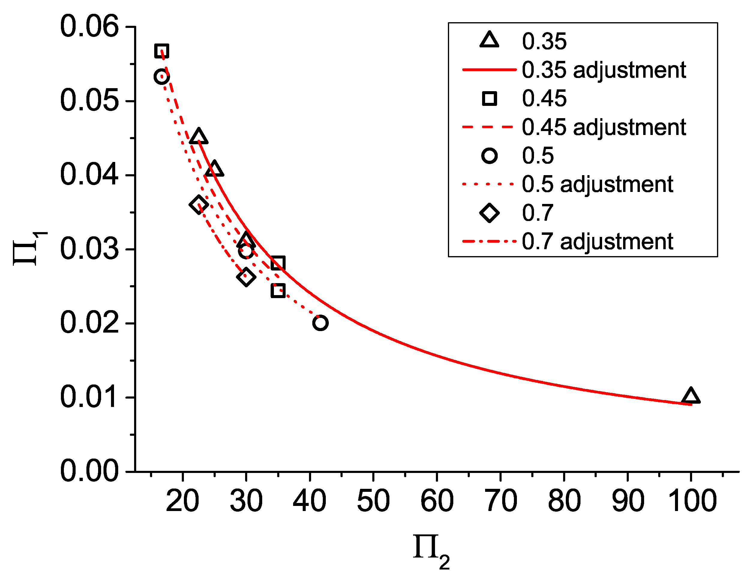
For the second estimated forming time $t_o^{II}$, since the values of m are habitually distributed within a range between 0.3 and 0.7, four groups are formed corresponding to values of the parameter close to 0.35, 0.45, 0.5 and 0.7, respectively. This way of operating is due to the fact that there are few trials that can be associated to the same value of m. To this end,

Table 2. Sets of parameter m with materials and their test conditions.

m	PbSn60	ZnAl22	AZ31	AA5083	Alnovi-U	Ti-6Al-4V
0.35	50 °C (0.364)	270 °C (0.35)	450 °C (0.391)			800 °C (0.382)
0.45			520 °C (0.457)		450 °C (0.439)	900 °C (0.43)
0.5			450 °C (0.544)	450 °C (0.5)	500 °C (0.5)
0.7			520 °C (0.723)			850 °C (0.703)

shows the four groups including the information of temperature and the exact value of m, according to the analysed tests from the Table 1.

Figure 3 shows the total amount of tests grouped in the four set of m values, plotting the regression curves that better fit between the points by power law functions. These power law functions are:

$$m\approx 0.35⟹{\Pi }_1=1.242{\Pi }_2^{-1.068}$$

(24)

$$m\approx 0.45⟹{\Pi }_1=1.051{\Pi }_2^{-1.063}$$

(25)

$$m\approx 0.5⟹{\Pi }_1=0.980{\Pi }_2^{-1.034}$$

(26)

$$m\approx 0.7⟹{\Pi }_1=1.105{\Pi }_2^{-1.099}$$

(27)

Based on these four expressions, the dimensionless function $\Phi$ can be generalised as

$$\frac{t_o{q}_o}{{\mu }_{ao}}=\Phi (AR,m)=\Xi \left(m\right)·A{R}^{\Psi \left(m\right)}$$

(28)

where the two functions $\Xi \left(m\right)$ and $\Psi \left(m\right)$, based on the coefficients of the Equations (24)–(27), can be written as cubic polynomial functions

$$\Xi \left(m\right)=1.269+3.487m-15.242m^2+14.146m^3$$

(29)

$$\Psi \left(m\right)=-1.423+1.639m-1.735m^2+0.110m^3$$

(30)

Thus, the Equation (28) can be applied to estimate the forming time as

$$t_o=\frac{{\mu }_{ao}}{q_o}\Xi \left(m\right)·A{R}^{\Psi \left(m\right)}$$

(31)

$$t_o^{II}=\sqrt[m]{\frac{K}{q_o}\Xi \left(m\right)·A{R}^{\Psi \left(m\right)}}$$

(32)

This expression is consistent with the proposed forming time calculation $t_f$ by Enikeev and Kruglov [17]

$$t_f=2I_m\sqrt[m]{\frac{K}{q_o}\frac{2}{AR}}$$

(33)

where $I_m$ refers to an integral, that can be calculated numerically, in which the upper bound is the value of m. This latter expression was obtained on the basis of the membrane theory and applying geometrical relationships, reporting a mean error of 15%.

The comparison of both estimated forming times is shown in

Table 3. Results of estimated forming time using (23) and (32) compared to the experimental forming time.

Material	Temp. (°C)	Pressure (MPa)	${\mathit{t}}_{\mathit{o}}^{\mathit{I}}\left({\mathbf{\Phi }}^{*}\right)$	${\mathit{t}}_{\mathit{o}}^{\mathbf{II}}\left(\mathbf{\Phi }\right)$	${\mathit{t}}_{\mathbf{exp}}$(s)
ZnAl22	270	0.4	255	362	365
		0.6	113	161	160
		0.8	64	91	87
AA5083	450	0.29	1059	998	1138
		0.56	177	167	142
		0.90	37	35	26
PbSn60	50	0.06	123	127	122
		0.07	80	83	99
		0.08	56	58	69
		0.09	40	42	50
		0.10	31	33	45
Alnovi-U	450	0.6	881	1079	1045
		0.75	530	650	603
		0.9	350	428	436
	500	0.3	2157	2226	2499
		0.4	1214	1252	1189
		0.5	777	801	668
		0.6	285	252	260
		0.7	224	198	199
		0.8	182	161	153
AZ31	450	0.2	3554	3153	3407
		0.25	2358	2092	2435
		0.35	1270	1127	1185
		0.5	394	503	423
	520	0.11	2786	2431	2206
		0.17	1526	1331	1307
		0.16	884	944	809
		0.29	241	257	200
Ti-6Al-4V	800	1.25	4590	6291	5878
		1.5	2848	2903	3671
		1.75	1902	2607	2924
	850	0.5	5361	4794	4597
		1.0	2000	1788	1815
		1.5	1123	1004	924
	900	0.5	1232	1408	1500
		0.7	563	644	678
		1.0	246	281	291

. It can be seen that the inclusion of the dependence with m in the process law allows us to obtain a significant improvement in the results, from a mean error of 16% to a 10% when m is considered.

This improvement is also shown in the Figure 4 where a histogram of the deviations of both estimated forming times from the experimental value is represented. For $t_o^I$, most of the values of deviation are between 15% and 20%, while for $t_o^{II}$, most of the deviations are less than 5%. This improvement is obtained regardless of the fact that the four fitting power functions are formed by a few number of tests and, most of then condensed in a range of $AR$ between 20 and 40. Despite that, the DA procedure has been able to provide an expression of the forming time for any material developing superplastic behaviour on a free-inflation test.

Within the set of test of the Table 1, those for Alnovi-U material at 500 °C between 0.6 and 0.8 MPa possesses a value of m that hinders its use in any of the four groups. However, the mean error obtained for these tests is lower than 5%.

It is important to retain the exponents from both estimator time expressions (23) and (32), $-0.984$ and $\Psi \left(m\right)$ in our work, in order to maintain the mean error closer to 10%, even though we could be tempted to approximate those two values to $-1$ in both cases.

Larger deviations between experimental forming time and our estimations may have two main sources of error. Firstly, it has to be reminded the way in which $\Xi \left(m\right)$ and $\Psi \left(m\right)$ are calculated, setting groups of tests with similar values of m, and applying a range of $AR$ between 20 and 40. Consequently, a better estimation requires to get larger groups of experiments over a wider range of $AR$ in which the materials possess the same value of m. Secondly, the behaviour of the materials for different pressures, i.e., different strain rates, have been approximated using a single power-law constitutive equation with the expression (1). Therefore, it is normal to observe that the constitutive equation diverges from the actual behaviour when the strain rates are close to the extremes of the test range.

4. Conclusions

The application of the DA and making use of the Buckingham $\Pi$ theorem was introduced as an accurate tool for the study of superplastic processes. A mathematical framework was developed, specifying to the type of behaviour normally presented in superplasticity. This particularisation requires to change the way in which the material is characterised by unifying its description into a single strain-rate dependent variable called apparent viscosity. The DA was applied to free-inflation tests in order to obtain the law process from which to write forming time estimator expressions. The whole system was reduced from six dimensional variables to the study of only three dimensionless variables. Therefore, the forming time can be expressed as a function of a geometric parameter, $AR$, and a material parameter, m. From this relationship, two different forming time estimator are compared, depending on whether the influence of the material parameter is neglected or not. For the former estimator, a mean error of 16% is obtained, while this value is reduced to 10% when the influence of m is taken into account. Other works from different authors provided similar expressions through the mathematical development of the membrane theory equations, reporting a mean error of 15%.

Therefore, results show that DA opens the door not only to test SPF processes in down-scale dimensions, but also to apply to different materials as long as the similarity principles for geometry, process and material are fulfilled. For instance, parts formed superplastically from a titanium alloy might be analysed studying a down-scale model on a different material like a magnesium alloy, which thermal and mechanical requirements, as well as cost, are considerably lower.

References

- Barnes, A.J. Superplastic Forming 40 Years and Still Growing. J. Mater. Eng. Perform. 2007, 16, 440–454. [Google Scholar] [CrossRef]
- Friedman, P.A.; Luckey, S.G.; Copple, W.B.; Allor, R.; Miller, C.E.; Young, C. Overview of superplastic forming research at Ford Motor Company. J. Mater. Eng. Perform. 2004, 13, 670–677. [Google Scholar] [CrossRef]
- Hefti, L.D. Advances in fabricating superplastically formed and diffusion bonded components for aerospace structures. J. Mater. Eng. Perform. 2004, 13, 678–682. [Google Scholar] [CrossRef]
- Hefti, L.D. Commercial Airplane Applications of Superplastically Formed AA5083 Aluminum Sheet. J. Mater. Eng. Perform. 2006, 16, 136–141. [Google Scholar] [CrossRef]
- Bonet, J.; Wood, R.D.; Said, R.; Curtis, R.V.; Garriga-Majo, D. Numerical simulation of the superplastic forming of dental and medical prostheses. Biomech. Model. Mechanobiol. 2002, 1, 177–196. [Google Scholar] [CrossRef]
- Sorgente, D.; Palumbo, G.; Piccininni, A.; Guglielmi, P.; Aksenov, S.A. Investigation on the thickness distribution of highly customized titanium biomedical implants manufactured by superplastic forming. CIRP J. Manuf. Sci. Technol. 2018, 20, 29–35. [Google Scholar] [CrossRef]
- Hefti, L.D.; Hefti, L.D. Innovations in the Superplastic Forming and Diffusion Bonded Process. J. Mater. Eng. Perform. 2008, 17, 178–182. [Google Scholar] [CrossRef]
- Ortiz, A.A.; Gago, J.; Sanchez, P.; Gil, V.; Rubio, L. Technical and industrial approaches for super plastic forming and diffusion bonding (SPF/DB) titanium alloy leading edge manufacturing. Mater. Werkst. 2014, 45, 785–792. [Google Scholar] [CrossRef]
- Xun, Y.W.; Tan, M.J. Applications of superplastic forming and diffusion bonding to hollow engine blades. J. Mater. Process. Technol. 2000, 99, 80–85. [Google Scholar] [CrossRef]
- Totten, G.; Funatani, K.; Xie, L. Handbook of Metallurgical Process Design; Materials Engineering; Marcel Dekker lnc.: New York, NY, USA, 2004. [Google Scholar]
- Aksenov, S.A.; Kolesnikov, A.V.; Mikhaylovskaya, A.V. Design of a gas forming technology using the material constants obtained by tensile and free bulging testing. J. Mater. Process. Technol. 2016, 237, 88–95. [Google Scholar] [CrossRef]
- Franchitti, S.; Giuliano, G.; Palumbo, G.; Sorgente, D.; Tricarico, L. On the optimisation of superplastic free forming test of an AZ31 magnesium alloy sheet. Int. J. Mater. Form. 2008, 1, 1067–1070. [Google Scholar] [CrossRef]
- Antoniswarny, A.; Taleff, E.; Hector, L.; Carter, J. Plastic deformation and ductility of magnesium AZ31B-H24 alloy sheet from 22 to 450 °C. Mater. Sci. Eng. A 2015, 631, 1–9. [Google Scholar] [CrossRef]
- Jovane, F. An approximate analysis of the superplastic forming of a thin circular diaphragm: Theory and experiments. Int. J. Mech. Sci. 1968, 10, 403–427. [Google Scholar] [CrossRef]
- Belk, J.A. A quantitative model of the blow-forming of spherical surfaces in superplastic sheet metal. Int. J. Mech. Sci. 1975, 17, 505–511. [Google Scholar] [CrossRef]
- Yu-Quan, S.; Jun, Z. A mechanical analysis of the superplastic free bulging of metal sheet. Mater. Sci. Eng. 1986, 84, 111–125. [Google Scholar] [CrossRef]
- Enikeev, F.U.; Kruglov, A.A. An analysis of the superplastic forming of a thin circular diaphragm. Int. J. Mech. Sci. 1995, 37, 473–483. [Google Scholar] [CrossRef]
- Giuliano, G.; Franchitti, S. On the evaluation of superplastic characteristics using the finite element method. Int. J. Mach. Tools Manuf. 2007, 47, 471–476. [Google Scholar] [CrossRef]
- Huh, H.; Choi, T.H. Modified membrane finite element formulation for sheet metal forming analysis of planar anisotropic materials. Int. J. Mech. Sci. 2000, 42, 1623–1643. [Google Scholar] [CrossRef]
- Bonet, J.; Wood, R.D.; Collins, R. Pressure-control algorithms for the numerical simulation of superplastic forming. Int. J. Mech. Sci. 1994, 36, 297–309. [Google Scholar] [CrossRef]
- Bonet, J.; Gil, A.; Wood, R.D.; Said, R.; Curtis, R.V. Simulating superplastic forming. Comput. Methods Appl. Mech. Eng. 2006, 195, 6580–6603. [Google Scholar] [CrossRef]
- Alabort, E.; Putman, D.; Reed, R.C. Superplasticity in Ti–6Al–4V: Characterisation, modelling and applications. Acta Mater. 2015, 95, 428–442. [Google Scholar] [CrossRef] [Green Version]
- García-Barrachina, L.; Gámez, A.J. A forming time estimator of superplastic free bulge tests based on dimensional analysis. Int. J. Mater. Form. 2020. [Google Scholar] [CrossRef]
- Padmanabhan, K.A.; Vasin, R.A.; Enikeev, F.U. Superplastic Flow: Phenomenology and Mechanics; Springer: Berlin, Germany, 2001; pp. 311–324. [Google Scholar]
- Zohuri, B. Dimensional Analysis Beyond the Pi Theorem; Springer: Cham, Switzerland, 2017. [Google Scholar] [CrossRef]
- Lemons, D.S. A Student’s Guide to Dimensional Analysis; Cambridge University Press: Cambridge, UK, 2017. [Google Scholar] [CrossRef] [Green Version]
- Tan, Q.M. Dimensional Analysis: With Case Studies in Mechanics; Springer: Berlin/Heidelberg, Germany, 2011. [Google Scholar] [CrossRef]
- Szirtes, T.; Rózsa, P. Applied Dimensional Analysis and Modeling; Elsevier Science & Technology: Oxford, UK, 2007. [Google Scholar] [CrossRef]
- García-Barrachina, L.; Gámez, A. Superplastic Materials Characterisation Based on Free-Bulge Tests. Solid State Phenom. 2020, 306, 15–22. [Google Scholar] [CrossRef]
- Delaplace, G. (Ed.) Dimensional Analysis of Food Processes; Elsevier: Oxford, UK, 2015. [Google Scholar] [CrossRef]
- Jarrar, F.S.; Abu-Farha, F.; Hector, L.G.; Khraisheh, M.K. Simulation of high-temperature AA5083 bulge forming with a hardening/softening material model. J. Mater. Eng. Perform. 2009, 18, 863–870. [Google Scholar] [CrossRef]
- Ramos, R.E.; Prada, J.C.G.; Giuliano, G. Análisis de las Características Mecánicas de la Superplasticidad: Aplicación a la Aleación de PbSn60. Master’s Thesis, Universidad Carlos III, Madrid, Spain, 2011. In Spanish. [Google Scholar]
- Sorgente, D.; Tricarico, L. Characterization of a superplastic aluminium alloy ALNOVI-U through free inflation tests and inverse analysis. Int. J. Mater. Form. 2014, 7, 179–187. [Google Scholar] [CrossRef]
- Sorgente, D.; Palumbo, G.; Piccininni, A.; Guglielmi, P.; Tricarico, L. Modelling the superplastic behaviour of the Ti6Al4V-ELI by means of a numerical/experimental approach. Int. J. Adv. Manuf. Technol. 2017, 90. [Google Scholar] [CrossRef]
Figure 1.
Geometrical scheme of a free-inflation test.
Figure 2.
vs. . For each material and temperature, a mean value of is plotted. Fitting power function is added.
Figure 3.
vs. . Fitting power law functions are extracted for the four groups.
Figure 4.
Histogram of the deviation of the estimated forming times from the experimental values.