
Evaluation of Melting Efficiency in Cold Wire Gas Metal Arc Welding Using 1020 Steel as Substrate

Centre for Advanced Materials Joining (CAMJ), University of Waterloo, 200 University Avenue West, Waterloo, ON N2L 3G1, Canada
*
Author to whom correspondence should be addressed.
Metals 2024, 14(4), 484; https://doi.org/10.3390/met14040484
Submission received: 8 March 2024
/
Revised: 15 April 2024
/
Accepted: 19 April 2024
/
Published: 21 April 2024
(This article belongs to the Special Issue Editorial Board Members’ Collection Series: Additive Manufacturing Technology)
Abstract
:A key welding parameter to quantify in the welding process is the ratio of the heat required to melt the weld metal versus the total energy delivered to the weld, and this is referred to as the melting efficiency. It is generally expected that the productivity of the welding process is linked to this melting efficiency, with more productive processes typically having higher melting efficiency. A comparison is made between the melting efficiency in standard gas metal arc welding (GMAW) and cold wire gas metal arc welding (CW-GMAW) for the three primary transfer modes: short-circuit, globular, and spray regime. CW-GMAW specimens presented higher melting efficiency than GMAW for all transfer modes. Moreover, an increase in plate thickness in the spray transfer regime caused the melting efficiency to increase, contrary to what is expected.
1. Introduction
Welding plays a critical role in the overall productivity of manufacturing, as well as the reliability of structures. During welding, residual stress and distortion cause many issues in assembly, and these are caused by excess heat transferred to the workpiece, not required for melting material. Thus, it is desirable that most of the power delivered during welding be directed towards melting and depositing metal.
The melting efficiency specifically measures how much of the effective power delivered to the substrate is used for melting filler material and base metal, thus creating a diluted weld pool, which is a mixture of filler and parent material during welding. Several studies reported the melting efficiency of standard gas metal arc welding (GMAW) as a function of process parameters. Perhaps one of the first studies by Wells [1] reported that melting efficiency is a direct function of the ratio , where is the metal thermal diffusivity, v is the travel speed, and w is the weld pool width. In this work, the melting efficiency increases with the travel speed.
DuPont and Marder [2] systematized their findings on melting efficiency and proposed a maximum limit for this variable for different welding processes. Hirata et al. [3] studied the melting efficiency for GMAW using different plate thicknesses and concluded that the arc current intensity and plate thickness affect its value, where higher current gradients around the weld pool will increase melting efficiency, if the thermal gradient is high, and thinner plates decrease heat losses, thereby increasing the melting efficiency.
Reis et al. [4] employed gas tungsten arc welding (GTAW) for three different metals and concluded that austenitic stainless steel presents higher melting efficiency than plain carbon steel and aluminum alloys. Recently, Hackenhaar et al. [5] studied the melting efficiency for GMAW using two geometry configurations and concluded that the melting efficiency in GMAW strongly depends on the heat transfer regime, where 3D heat transfer generally offers lower melting efficiency compared to 2D heat transfer regimes. Furthermore, Sing et al. [6] reported the crucial influence of the thermal properties (particularly the latent heat of fusion) on melting efficiency, reporting calculated values raging from 24.8 to 56%, which successfully validated, with errors less than 8.3%, his numerical simulation for submerged arc welding (SAW).
Recently, Assunção and Bracarense [7] investigated a strategy to increase melting efficiency in under-water flux-cored arc welding (UW-FCAW). They found that using a dry contact tip caused the melting efficiency increase to approximately, on average, 0.33 compared to conventional UW-FCAW, which presented on average a melting efficiency of 0.25. Bal et al. [8] used finite element analysis (FEA) to assess melting efficiency on laser beam welding of Hastelloy C-276 in the bead-on-plate configuration. They found that the melting efficiency increased with an increase in nominal heat input (J/mm). They reported, using numerical analysis, a maximum melting efficiency of 70% for a heat input of 10 J/mm versus a melting efficiency of approximately 20% for a heat input of 70 J/mm.
Cold wire gas metal arc welding (CW-GMAW) is a welding process derived from standard GMAW that aims to improve deposition rate (kg/h) while keeping the nominal heat input constant [9]. The process has shown some interesting properties, such as precise geometrical control during additive manufacturing and a reduction in dilution while achieving a deposition rate of 9.57 kg/h [10]. Moreover, the use of CW-GMAW reduces heat-induced distortion [11]. Furthermore, this process has been successful in the additive manufacturing of duplex stainless steel parts, while reducing the Nickel equivalent [12]. Lastly, CW-GMAW with wire pulsation was used to limit the heat imposed on a substrate while reducing the coarse-grained heat-affected zone (CGHAZ) [13].
The studies in the literature concentrate on standard GMAW or standard GTAW; however, other derivative processes were developed in the last years which were not studied. Among these is cold wire gas metal arc welding (CW-GMAW). This process has been successfully applied for wire arc additive manufacturing (WAAM) [10]; however, there is a scarcity of data regarding melting efficiency in the contemporary literature. The present work aims to determine the melting efficiency of CW-GMAW for the three natural transfer modes (short-circuit, globular, and spray) while welding plain carbon steel and determine the effect of plate thickness on melting efficiency. Although the concept of melting efficiency is not new, there is no work in the literature that deals specifically with melting efficiency applied to CW-GMAW. As CW-GMAW is a suitable method compared to wire arc additive manufacturing (WAAM) given its improved deposition rate and its suppression of wire arc wandering [14], this study details the effect of different welding parameters in CW-GMAW on the amount of heat specifically used to melt the feed wire, i.e., on melting efficiency. The data regarding thermal efficiency for the conditions reported here were taken from prior work [15]. Additionally, the melting efficiency results determined by two methods are compared, and a methodology to determine the melting for a range of arc powers is discussed.
2. Experimental Methodology
2.1. Welding Procedures and Materials
Bead-on-plate steel welds were manufactured using a Lincoln R500 welding power source and Fanuc ArcMate 120i robotic arm. The welding power source operated in constant voltage (CV), which means that voltage is not set at the beginning in the welding power source but measured during welding. The cold wire feed angle was constant and equal to 49 degrees, and the process parameters were varied so that the welds were produced using the three natural transfer modes: short-circuit, globular, and spray. The plain carbon steel welding plates (AISI 1020) used were 6.35 mm and 9.53 mm thick. The plates were welded on top of a water-flow calorimeter (described in prior work [15]) in which the back of the plate was directly cooled with water in order to measure the energy transferred to the substrate during welding. The welding wire used in this work was ER70S-6, with 1.2 and 0.9 mm diameters used, respectively, as the electrode wire and cold wire. Table 1 summarizes the calorimeter parameters used in this work for the three natural transfer modes: wire feed speed (WFS), voltage (V), welding travel speed, contact-tip to workpiece distance (CTWD), and cold wire mass feed rate as the mass percentage of the electrode WFS. Table 1 summarizes the welding parameters used in this study. The shielding gas mixture used was Ar-25 % at a flow rate of 19 L/min.
Each welding condition was performed using three (3) replicates (8 inches [203 mm] × 5 inches [127 mm]). Each sample replicate was cut into three separate locations, equally distanced to measure the bead areas and calculate melting efficiency. This resulted in the areas used to calculate melting efficiency (using the first approach) being reported as an average of nine (9) values. However, for the values of relative plate thickness which are mainly dependent on the net value of heat input, they were calculated as an average of two (2) values, since each sectioned sample was manufactured with the same thermal efficiency. Furthermore, to represent the measurement errors in a more meaningful manner, given a lower number of replicates, 95% confidence intervals are used in this work as error bars, to represent the values of melting efficiency, Rykalin number, and Christensen number. However, the errors of relative plate thicknesses, given their semi-quantitative natures (particularly using the AWS approach to avoid the intermediate values of , described in Section 2.4) are reported using standard deviations.
During welding, the current and voltage were acquired for 2 s at a frequency of 10 kHz to measure the average voltage (U), average current (I), average power (P), and nominal heat input (E) in agreement with the algorithm proposed by Joseph [16], using:
where and refer to the instantaneous values of voltage and current, respectively, and v refers to the travel speed.
2.2. Thermal Efficiency Measurements
The thermal efficiency was measured using a water plate calorimeter, as described in prior work [15]. Each thermal efficiency experiment was replicated three times to achieve confidence in the results. The calorimeter block measured 200 × 127 × 40 mm with inlet and outlet diameters of 19.05 mm (Figure 1). Four thermocouples in the water inlet and in the outlet were used to measure the water temperature difference in order to calculate the thermal efficiency; further details on the calorimeter set-up and the thermal efficiency calculations can be found in prior work.
The calorimeter flow rate used in the experiments was just 5 L/min. Varying cold wire feed rates were employed at 60% (for intermediate) and 100% and 120% (high), respectively, for short-circuit and globular/spray metal transfer regimes. The parameters used in the calorimeter tests are summarized in Table 2.
The length of the weld beads was 120 mm. With the results of average power, thermal efficiency was calculated using Equation (5):
where is the specific heat of water at 290 K, is the welding time, is the average water mass rate, and is the water temperature difference between the outlet and inlet. The values of the constants used in this work can be found in prior work [15].
2.3. Melting Efficiency Calculation
Melting efficiency refers to the amount of energy used to specifically create the weld bead, and it indicates how much of the heat is effectively transferred to the workpiece. It is generally understood that the maximum value of melting efficiency, considering 2D and 3D heat transfer regimes, corresponds to 50% of the energy transferred by the electric arc to the substrate during welding [17]. Two approaches are found in the literature to calculate melting efficiency. The first approach is mainly experimental since it relies on the determination of thermal efficiency through calorimetry, dimensional measurements of the cross-section, and the calculated base and filler metal volumetric melting enthalpies. The second approach relies on the experimental determination of thermal efficiency and theoretical calculations.
2.3.1. First Approach
Melting efficiency was defined by DuPont and Marder [2] as the ratio:
where is the area of the weld bead due to the base metal, v is the travel speed, is the volumetric melting enthalpy of the base metal, is the area of the bead due to the filler metal, and is the volumetric enthalpy of the filler metal. The values of volumetric melting enthalpy (H) used in this work are an approximation based on the melting temperature of the base and filler metals, respectively. Hackenhaar et al. [5] reports the relation between H and melting temperature () as:
In Equation (7), is given in Kelvin. The values of melting temperature for AISI 1020 steel and ER70S-6 are 1775 and 1538 K, respectively [5]. Taking these values of melting temperatures and inserting them into Equation (7) gives the values of and , which are 10.5 J/m3 and 7.88 J/m3 [5], respectively. Figure 2 shows the schematic representation of a cross-sectioned weld bead to illustrate the different parts of the weld cross-section used to calculate melting efficiency experimentally.
2.3.2. Second Approach
The second approach relies on the determination of two dimensionless numbers called the Rykalin number (Ry) and the Christensen number (Ch); both numbers were originally proposed by Fuerschbach and Eisler [18]. These dimensionless numbers can be written as:
where is the net heat transferred to the workpiece, v is the travel speed, is the thermal diffusivity of the base metal, and A is the cross-sectional area of the weld bead, which is . In this work, of the base metal (plain carbon steel at 300 K) is taken to be equal to 17.7 mm2/s, cf. Table A1 in Incropera et al. [19]. From Equations (8) and (9), the melting efficiency can be written as:
This approach still needs the value of the thermal efficiency of the process to be determined through calorimetry so that can be calculated.
2.4. Relative Plate Thickness
The relative plate thickness () is a dimensionless number that can be derived from the cooling rates of bead-on-plate welds based on the Rosenthal equation [20], and it indicates the heat transfer regime in which the weld was performed. The following equation is used to calculate this parameter:
where h is the workpiece/plate thickness, is the density of the base metal, is the specific heat of the base metal, and is the upper temperature which is used to calculate relative plate thickness. In this work, for the melting temperature of the base metal (AISI 1020 steel), is the room temperature, and is the heat transferred to the workpiece. If , there is a 3D heat transfer regime, while if , there is 2D heat transfer regime. Otherwise, if , the heat transfer regime is said to be intermediate.
The relative plate thickness determines the heat transfer regimes during welding. These heat transfer regimes, which can be 2D (bidimensional) or 3D (tridimensional), do not solely depend on the plate thickness of the welding substrate but also on the relative substrate thickness to welding heat source dimensions. The interplay of these variables (thickness of the substrate and heat source shape) is what will ultimately determine the heat transfer regime during welding.
However, there are many practical situations in which assumes intermediate values, and so the Welding Handbook of the American Welding Society (AWS) [20] recommends the arbitrary value of 0.75 to avoid the intermediate condition. Therefore, if , there is a 3D heat transfer regime; otherwise, if , there is a 2D heat transfer regime.
The conditions explored in this work correspond, in the short-circuit transfer regime, to the following range interval: ; for the globular transfer regime, the interval corresponds to ; while for the spray transfer regime, the values of correspond to the following interval: .
2.5. Metallographic Procedure
After welding, three cross-sections of each replicate were sectioned and subjected to standard metallographic procedure (grinding with sandpaper until grit 1200 and subsequently polishing with a 1.0- and 0.5-micron alumina ) water solution). The weld cross-sections were etched with a 5% Nital solution. The cross-sectional areas, and , were measured using the ImageJ software, version 1.53k.
3. Results
3.1. Electrical Data
Table 3, summarizing the average electrical data, is presented here, as well the values of the average nominal heat input. These data clearly distinguish the three natural transfer modes in terms of their nominal heat input, where low, intermediate, and high heat input values are attributed to the short-circuit, globular, and spray transfer regimes, respectively. Further details concerning oscillograms and cyclograms for the experimental conditions reported in this work can be seen in prior work [15], where all data regarding the electrical parameters for the welding conditions are presented.
3.2. Cross-Sections
Figure 3 shows the cross-sections of the welds produced in the short-circuit, globular, and spray regimes, which were welded on plates on the calorimeter set-up described in Figure 1. Although the parameters used here are similar to those employed in prior work [21], the influence of the water flow rate used in the calorimeter was not characterized in terms of the effect on bead profile. This influences the heat boundary conditions, leading to the shallowing of the weld pool. This decrease in weld pool size affects its ability to accommodate extra cold wire feed, therefore increasing the occurrence of welding discontinuities, particularly in low-energy transfer modes, such as the short-circuit regime. For instance, the welds produced in the short-circuit transfer mode contained defects such as a lack of fusion (Figure 3a—CW-60%/Test-2) and inclusion (Figure 3a—CW-100%/Test-1).
However, the cross-sections of the globular regime and spray transfer do not present such defects. These defects come from the high cooling provided by the calorimeter which affects the accommodation of cold wire in the welding pool, as discussed above. In the globular and spray regimes, the energy level in the weld pool is higher than in the short-circuit regime, and so those regimes are not significantly affected by the calorimeter cooling effect, as shown in Figure 3b,c, where it can be seen that such defects did not occur.
The GMAW macrograph shown in Figure 3c is different from the other GMAW conditions (shown in Figure 3a,b) because the transfer mode is different. In Figure 3c, it is spray transfer, and in Figure 3a,b, it is the short-circuit and globular transfer modes, respectively. Comparing the GMAW condition in Figure 3c and also the CW-GMAW conditions in Figure 3c, one notes the size of the of the heat-affected zone (HAZ) that extends through the thickness in GMAW but not in the CW-GMAW conditions. This is consistent with a change in cooling rate regime, 2D (GMAW thin plate) versus 3D (GMAW thick plate), as shown in Table 4 in the manuscript. Moreover, we compare the condition GMAW thin plate (2D) to the other 2D condition, for instance, thin plate/CW-60% or thin plate/CW-120%, both shown in Figure 3c. One notes that the size of the HAZ is not the same. This is probably due to the changes induced in the heat source isotherms caused by the cold wire feed. This difference will be the object of future work and is out of the scope of the current study.
Another feature that the cross-sections reveal is the possible change in the heat transfer regime caused by the calorimeter parameters used in thin (6 mm) and thick (9.5 mm) plate conditions. Table 4 shows the heat transfer regime for all the conditions reported in this work and the actual values, between parentheses, of the relative plate thickness . These heat transfer regimes were calculated considering the threshold value of 0.75 (suggested by AWS, cf. Section 2.4), which means that if , a 3D heat transfer regime occurs; otherwise, if, however, , a 2D heat transfer regime takes place.
Welding in the short-circuit regime occurs in the 3D heat regime (cf. Table 4). This is consistent with assuming that the heat source is a point, in relation to the thickness of the welding substrate. Moreover, the standard deviation (data dispersion) for the same welding process condition (intra-class) assumes the values of 0.31, 0.37, and 0.37, respectively, for the standard GMAW, CW-60%, and CW-100%. This shows that an increase in plate thickness (thin to thick plate) affects data dispersion when comparing standard GMAW to CW-GMAW but does not exert influence when comparing CW-60% and CW-100%. Furthermore, when comparing the data among welding process conditions (inter-class), for instance, GMAW thin plate to CW-60% thin plate, the standard deviation is equal to 0.03, which is the same for all inter-class comparisons, keeping the plate thickness the same, except when comparing a standard GMAW thin plate to a CW-120% thin plate, where the dispersion is zero, and when comparing a standard GMAW thick plate to a CW-120% thick plate, where the standard deviation is 0.06. This indicates that the introduction of cold wire does not significantly alter the dispersion of the relative plate thickness data. Overall, the data indicate that plate thickness exerts a higher influence than cold wire feed rate on the dispersion of relative plate thickness for the short-circuit transfer regime, within the boundary of welding parameters investigated for this condition in this work.
The reported values of standard deviations for the relative plate thicknesses are based, as said in Section 2.1, on two replicates. And they are informed only to give an approximation of the cooling rate regime of the sample, since this regime can be determined by wide intervals, according to the AWS approach, which prescribes that if () then a 3D regime is characterized; otherwise, if (), then a 2D regime occurs. Therefore, these data only offer a semi-quantitative view. Particularly, about the short-circuit regime, the standard deviations are used only to show a higher dispersion within this metal transfer regime, comparing the standard GMAW and CW-GMAW conditions. Furthermore, we compare the standard deviations for different classes, for instance, keeping the plate thickness constant. One notes that the standard deviation between GMAW with a thin plate (, see Table 4) and CW-GMAW-60% with a thin plate (, see Table 4) is 0.03, as already noted. This information is discussed here to potentially stress that the cold wire feed alone cannot cause a change in the cooling rate mode. However, more research is needed on this matter and will be the object of future work.
In the globular transfer regime, however, the 3D heat regime only occurs when the thick plate condition is employed (Table 4); this means that, for thin plates (2D heat regime), the welding heat source behaves as a linear heat source. Again, we compare within the same welding process condition, just varying plate thickness (intra-class comparison). One can note that the standard deviation is, respectively, 0.30, 0.21, and 0.21 for the standard GMAW, CW-60%, and CW-120% conditions. The inter-class comparison of data (a comparison of different welding process conditions, keeping the plate thickness the same) accounts for the standard deviation of approximately 0.01 for all conditions, except when comparing a standard GMAW thick plate to CW-60% and CW-120% thick plates, which is 0.11. Again, in the globular transfer regime, the introduction of the cold wire feed does not affect the dispersion of relative plate thickness data so that this dispersion might alter the heat transfer regime; it was observed that the plate thickness exerts higher influence. In the spray transfer regime, the 3D heat transfer also occurs only when thick plates are used, while using thin plates leads to a 2D heat transfer regime (refer to Table 4). The dispersion of the relative plate thickness data is 0.21 (considering GMAW thin and GMAW thick plate conditions), 0.31 (considering CW-60% thin and CW-60% thick plate conditions), and 0.23 (considering CW-120% thin and CW-120% thick plate conditions). The dispersion of the data in an extra-class comparison (between different welding processes but keeping the plate thickness condition the same) for all experimental conditions falls within the rage of 0.00–0.02. The exceptions occur when comparing standard GMAW and CW-60% (both using thick plates)—in this case, the standard deviation is 0.09—and when comparing CW-60% and CW-120% (both using thick plates); for this situation, the standard deviation is 0.07. One can note that, again, the dispersion in the data caused by the cold wire feed is lower than the dispersion caused by the plate thickness change. Overall, in the spray transfer regime, the cold wire feed does not seem to affect the shape of the welding power source, which is mainly determined by the relation between the power source and substrate (plate thickness).
In summary, the data analyzed here show that for all the natural transfer mode regimes (short-circuit, globular, and spray) within the boundary of the welding parameters studied here (a welding power range of approximately 4 to 9.4 kW), the cold wire feed rate does not seem to significantly affect the shape of the welding heat power source (whether the power source will act as a point, linear, or volumetric power source, given the boundary conditions during the welding operation). This power source shape, even in CW-GMAW, is governed by the relationship between the heat source and substrate thickness, which is consistent with Rosenthal theory [22].
3.3. Melting Efficiency
3.3.1. Experimental Approach
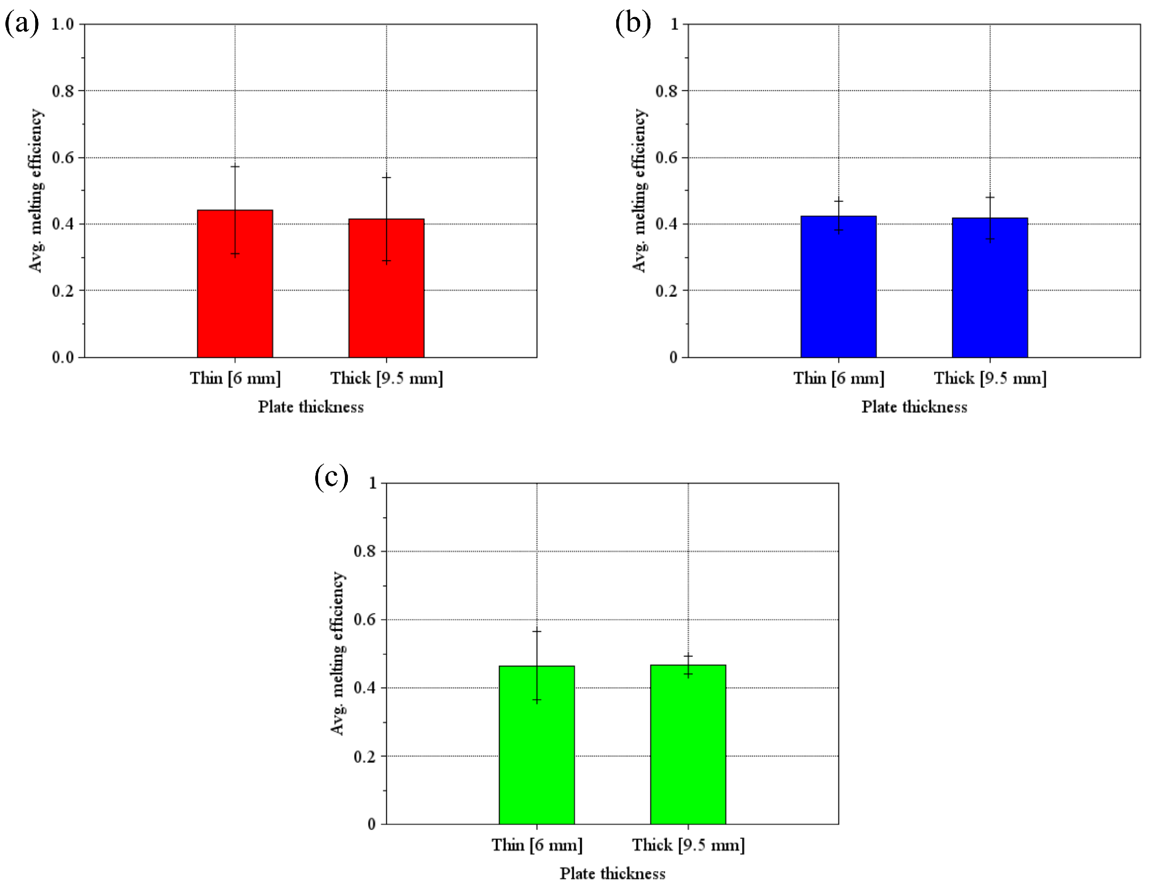
Figure 4 shows the melting efficiency determined using Equation (6) for the short-circuit metal transfer regime. The average value is never greater than 50%; however, the error bars pass this limit. In fact, the main reason for this large variation in melting efficiency for short-circuit transfer relates to the more irregular profiles, thus causing more scatter in the measured cross-sectional areas. The non-uniformity in bead shape during short-circuit transfer is well known, and that is still the case for these cold wire welds, as shown in prior work [15].
Generally, with the increase in plate thickness, the melting efficiency average decreases [23]. However, comparing the average melting efficiency in standard GMAW (Figure 4a) to CW-60% (Figure 4b), and CW-100% (Figure 4c), it can be seen that, for the thick plate (9.5 mm) condition, the melting efficiencies of CW-60% and CW-100% are higher than for standard GMAW. This is due to the increase in deposition in CW-GMAW compared to standard GMAW.
Figure 5 shows the melting efficiency determined using Equation (6) for the globular metal transfer regime. Differently from the short-circuit regime, the average melting efficiency is below 0.5, though the errors bars still pass that limit in standard GMAW. The trend is similar; the CW-GMAW achieves higher melting efficiency compared to standard GMAW.
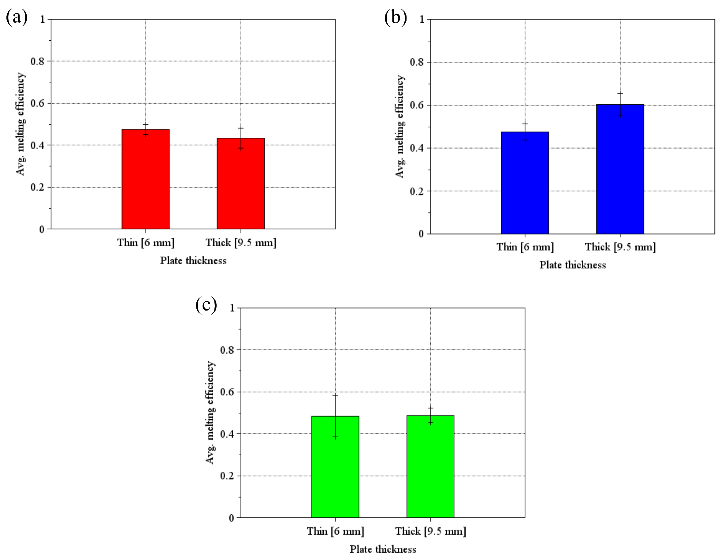
Figure 6 shows the melting efficiency determined using Equation (6) for the spray metal transfer regime. The limits of variation and the average of the melting efficiency for standard GMAW are now below the limit of 50%. In contrast, the CW-60% and CW-120% conditions present higher melting efficiency compared to standard GMAW, at least in terms of limits of variation. The previous trend remains: an increase in plate thickness, for the same condition, promotes an increase in melting efficiency.
In contrast to CW-60%, CW-120% does not exceed the 0.5 limit on average, though some of the individual tests do. This suggests that despite its higher deposition, the heat losses in CW-120% contribute to a lower melting efficiency. The sizes of error bars in some experimental conditions, for instance, in Figure 4, are due to the small number of replicates employed, only three. As a result, the credibility interval’s width increases, so the true value of melting efficiency is contained within them. Moreover, another reason why in Figure 4 the error bars are wider is that in the short-circuit regime, due to the alternance between high power (high current and voltage) and low power (short-circuit moment/arc extinguish), the energy transfer to the workpiece is not constant, which causes variability. This variability is not noted in globular and spray transfer, where the energy transfer does not vary. Another possible cause for the variability observed in Figure 4 is that the cooling provided by the calorimeter creates beads with discontinuities, as is shown in the macrographs reported in [15].
3.3.2. and Numbers for Different Cold Wire Feed Rates
Mendez et al. [24] pointed out that is directly linked to the temperature gradient inside the weld pool. They pointed out that can be used to characterize two welding regimes: (a) Regime I (higher numbers), where advection dominates over conduction, and (b) Regime II (lower numbers), where conduction dominates over advection. The aspect ratio of a welding pool, defined as its length over width, depends on its travel speed, which represents how fast or slow heat is transferred from the heating source to the substrate. The number can be interpreted as a measure of this trend, since it is proportional to the travel speed. Higher numbers () represent a fast heat source where the advective heat transfer dominates; otherwise, the conductive transfer dominates, for lower number (), over advection. These two regimes determine the aspect ratio of the weld pool: (a) higher travel speeds determine elliptical weld pools and higher numbers, which increase the aspect ratio, whereas (b) lower travel speeds determine circular weld pools, which decrease the aspect ratio.
Figure 7 shows the and the numbers for the short-circuit metal transfer regime calculated using Equations (5) and (6). The error bars point out that despite the variation in cold wire feed rate, both the and the numbers are statistically equal. This seems to indicate out there not statistically significant differences in terms of thermal gradient inside the weld pool while operating in the short-circuit transfer regime. However, this assertion must be taken with care since a wider range of parameters should be explored to assess the full range of the short-circuit metal transfer regime.
The number relates the inverse of the thermal diffusivity to the travel speed ratio and cross-sectional area of the weld bead, which scales with the deposition rate. This number relates how much of the cross-section area is derived from the heat that was not diffused through the base metal. In summary, a higher number means a higher fraction of heat is used for melting.
Figure 8 shows the and the numbers during globular metal transfer. The only difference in terms of statistical difference can be noted in Figure 8b, where the numbers for standard GMAW seem to be different. However, for both CW-60% and CW-120%, the values of are statistically indistinguishable from one another. This indicates that, again, there is no substantial difference in thermal gradients inside the welding pool for standard GMAW and CW-60% and CW-120% for globular transfer.
Figure 9 shows the Ry and the Ch numbers for the spray metal transfer regime. In Figure 9a, there is a difference from the previous trends; the Ry number for CW-60% on the thick plate (9.5 mm) condition presents a lower value compared to the same condition on the thin plate (6 mm). The reason behind this behavior is unclear and needs further work for elucidation.
3.3.3. Comparing Melting Efficiencies
Figure 10 shows the comparison of the melting efficiencies between the different transfer modes as calculated through Equation (6) (first approach) and Equation (10) (second approach). The first approach is presented in the abscissa, and the second approach is presented in the ordinate. The hybrid approach systematically overestimates the values of melting efficiency.
The reason for this relies on the hypothesis taken to determine the and numbers. These appear from the non-dimensionalization of the Rosenthal equation [22] for the temperature profiles on a semi-infinite plate, with no surface heat losses, assuming a constant moving small heat source [1,25]. While these numbers have been developed for heat sources without transfer of mass, they can be applied as well in situations where heat and mass transfer occur. For instance, these dimensionless numbers were applied to determine melting efficiency through an asymptotic solution and validated in welding with V-groove [25].
The authors reported that the overall error is below 10%. The data show that for all transfer mode regimes, the values of melting efficiency are displaced towards the ordinate (experimental values/first approach), which means that the data estimated by the second approach sub-estimate the values of melting efficiency, since they disregard heat losses through convection and radiation. Therefore, the values of melting efficiency determined through Equation (10) are overestimated due to the hypotheses considered when deriving the Rosenthal equation, which are steady state heat flow, point heat source, constant thermal properties (e.g., thermal diffusivity and thermal conductivity), no heat losses through the workpiece surface, and no convection or radiation [23]. Equation (6) does not consider all such hypotheses (e.g., point heat source and constant thermal properties). However, it implicitly considers heat losses since it requires the actual cross-section of the weld bead, with a size determined by the heat balance during the welding operation.
3.3.4. The Number Versus the Number
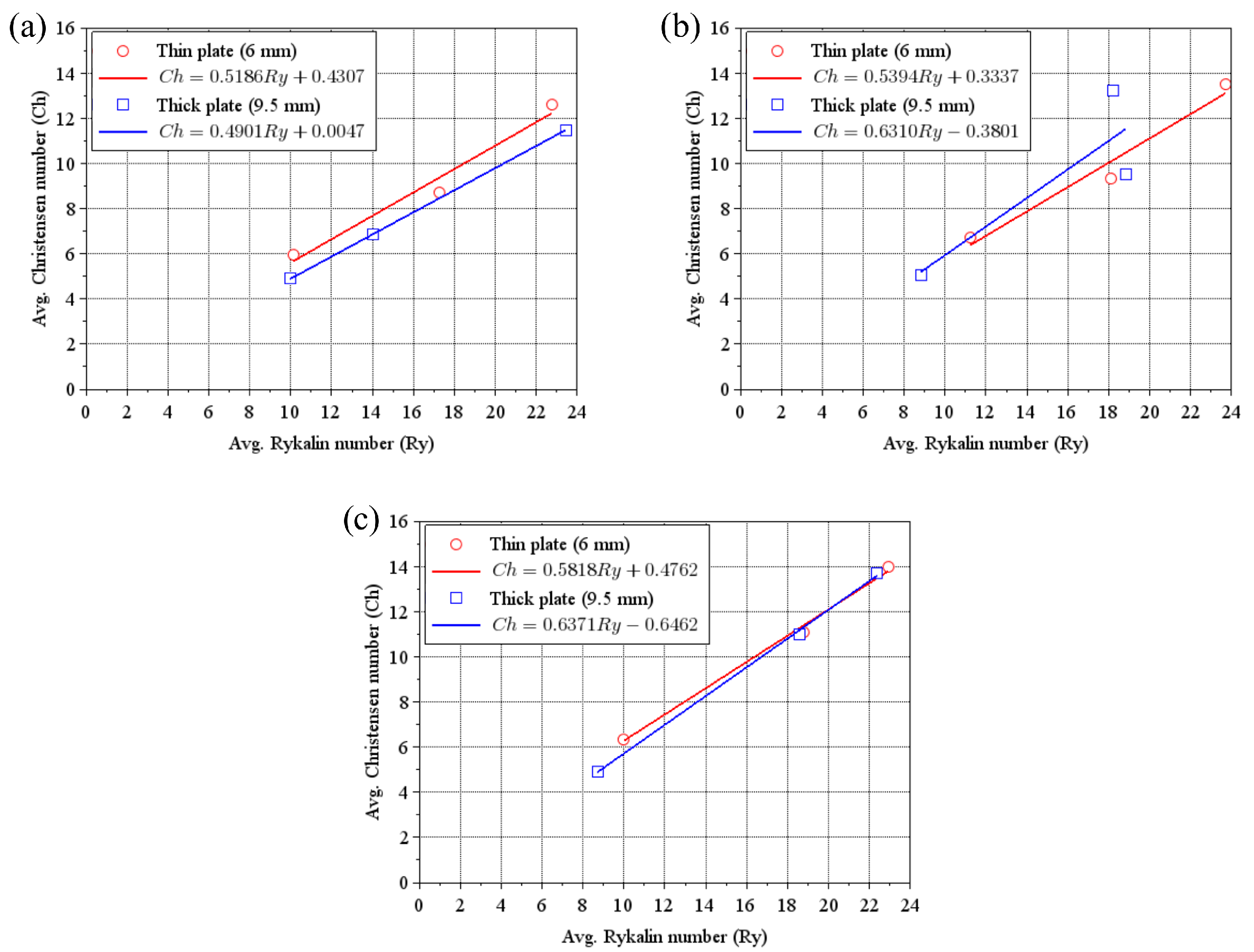
Figure 11 presents the plot of the versus the number for the conditions under study in this work, two basic geometries: thin and thick plates. It can be seen that the slope of the curve represents the melting efficiency for the range of parameters under study here for these two geometries. As mentioned in Section 3.3.3, the melting efficiencies determined by the ratio of by are overestimated. However, in principle, they constitute an upper limit to which the melting efficiency would tend to under ideal conditions. Therefore, this method can be used to ascertain the upper limit of the melting efficiency for a welding process over a wide range of parameters.
Figure 11a presents the versus the numbers for standard GMAW for thin and thick plates. The results show that the slopes are approximately the same, with the thin plate showing a slightly higher melting efficiency than the thick plate [26]. The values for all the conditions in Figure 11 can be seen in Table 5. The values in Figure 11a are higher than 0.95, which signifies that more than 95% of the variability in the data is explained by the proposed linear regression.
However, the value of a regression cannot be judged only by the values; the adjusted value (Adj. ), Table 5, does not take into account the increase in the number of factors in the regression and takes into account the size of the model [27]. In this case, the Adj. is also higher than 0.95, which indicates the robustness of the model. The exception is the intermediate cold wire feed rate (60%) thick plate (9.5 mm) condition, in which the Adj. is 0.748. This means that the model can account for only approximately 75% of the variability observed in the data. Moreover, the Adj. is only approximately 50%, which compromises the utilization of this particular equation for forecasting.
From Equation (10), when the Christensen number is plotted against the Rykalin number, the result will be a straight line with an angular coefficient numerically equal to the melting efficiency. This can be used to determine the melting efficiency over a range of Rykalin numbers, as in Figure 11. Even if the resulting straight line passes an intercept, its angular coefficient will be the same as that of a straight line through the origin of the axes.
For the conditions observed in Figure 11a, for a range of Rykalin numbers varying from 30 to 80, the melting efficiency is constant and equal to approximately 0.49 for both the thin and thick plate conditions. However, for Figure 11b, the melting efficiency for CW-60% varies from approximately 0.54 (thin plate) to approximately 0.63 (thick plate condition), for the same range of Rykalin numbers. In the case of high cold wire feed (100% and 120%), the melting efficiency is approximately 0.58 (thin plate condition), and it is approximately 0.64 in the thick plate condition.
For the range of Rykalin studied in this work, the melting efficiency has remained constant, differing only among the conditions with cold wire feed. Thus, as the Rykalin number is a function of the heat input, and this is determined by the instantaneous product of current and voltage. Therefore, if the welding conditions determine different pairs of Rykalin and Christensen numbers from those reported in this study, the angular coefficient of the straight line will change, representing different melting efficiencies.
Figure 11b shows the versus the number for CW-60% (intermediate cold wire feed rate). Differently from the standard GMAW, the thick plate solution has a melting efficiency higher than the thin plate solution. However, the of the thick plate is lower than 0.8, but considering the Adj. for the linear correlation is barely satisfactory. It seems that more points are required to determine a linear regression.
Figure 11c shows the versus the number for CW-100% and CW-120% (high cold wire feed rate). The data suggest that depending on the number two behaviors are possible: (a) for numbers lower than 60, the melting efficiency for thin plates is higher than for thick plates; (b) for numbers higher than 60, the melting efficiencies for thin and thick tend to be equivalent, and this is likely caused by the cold wire feed rate. The Adj. for high cold wire feed rate conditions is higher than 0.95, indicating that the model can reasonably explain the variation in the data.
4. Discussion
4.1. Confidence Intervals and Overlapping of Error Bars
The width of confidence intervals depends on three factors: (a) the variance of the sample, (b) the sample size, since precision varies non-linearly with sample size, and (c) the chosen level of confidence used to calculate the intervals [28]. The widest confidence intervals were observed in Figure 4, as the confidence level chosen and the sample size were the same for the other experimental conditions. Therefore, the increased interval width must come from the variability of the sample.
For instance, the standard GMAW operating in short-circuit regime presents for the thin plate condition a variance of 0.0049 and for the thick plate condition a variance of 0.0045. The CW-60% condition presents for the same experimental conditions, respectively, 0.0026 and 0.0091. It is hypothesized that the natural variance of the short-circuit regime, oscillating between zones of high and low heat input, associated with the cold wire feed increases variance in melting efficiency. In the other transfer mode regimes, as there is no intrinsic variability between low- and high-power states, the error bar width decreases. In these transfer modes (globular and spray), the width of the error is likely a function of small sample size, which was chosen as the minimum to establish a trend, three welds to measure thermal efficiency.
4.2. Using Melting Efficiency to Define Welding Processes
The welding process can be generally defined in terms of its thermal efficiency. For instance, during GTAW, welding steel with pure argon has a thermal efficiency ranging from 0.25 to 0.75 with mean of 0.40; meanwhile, for the case of GMAW, the same combination of base material and shielding gas has a thermal efficiency ranging from 0.66 to 0.70 with a mean of 0.70 [29]. Clearly, this is not an accepted approach to define welding processes, due to the range in which thermal efficiency varies, which can overlap for different processes, such as, for example, the GTAW and GMAW ranges discussed in this paragraph.
Melting efficiency, on the other hand, can be used to define a welding process more conveniently, since it tends to only one value and accounts for the energy directly used in melting during the welding operation. It is generally thought that the melting efficiency asymptotically approaches a maximum value of 0.5 for different welding parameters [2]. However, it seems that this value is never actually reached in standard welding processes, and the actual value of melting efficiency is constrained by the geometry of the welding joint, the cooling rate at the center of the weld bead, the material to be welded, the net power transferred to the substrate, and, when welding with filler metal, by the mass deposition rate.
These factors seem to cause the value of melting efficiency to fall below the limit of 0.5. However, the CW-GMAW can present a higher melting efficiency than the standard GMAW (cf. Figure 6b). In the other experimental conditions, the melting efficiency values between standard GMAW and CW-GMAW are comparable. The reason behind the difference shown in Figure 6b is still under study.
However, the limit of 0.5 in melting efficiency seems debatable; this value is a function of the reported range of thermal efficiency, 0.80 to 0.88 (), for standard GMAW, by DuPont and Marder [2]. Thus, for different values of thermal efficiency, the melting efficiency limit will be different from the limit reported. Some of the results presented here, even for standard GMAW (Figure 4a), have error bars reaching values higher than 0.5, for instance. This is likely due to measured values of thermal efficiency lower than the average of 0.84 (the average of the thermal efficiency range reported), which will increase the value of melting efficiency.
The number can be related to the internal thermal gradient inside the welding pool caused by the heat source using asymptotic and blending techniques [30]. These authors reported that, generally, the weld pool thermal gradient is inversely proportional to . Therefore, an increase in the number could mean a decrease in the thermal gradient, and vice versa. Only in CW-60% in the spray transfer regime in the thick plate (9.5 mm) condition (Figure 6b) is there a statistical difference in number compared to standard GMAW. In this condition, there is a decrease in the number, and, consequently, according to the relation above, there should be an increase in number. It appears that this variation in the thermal gradient within the welding pool leads to the increase in melting efficiency reported in Figure 6b.
The welding pool thermal gradient can be linked to the cooling rate through the following relation: . As the travel speed v is constant, it will follow that the thermal gradient is directly proportional to the cooling rate. The cooling rate regime can occur in two distinct modes, 2D or 3D. It can be demonstrated that the 3D regime cooling rate is higher than the 2D regime cooling rate. Then, the welds in Table 5 that experience a 3D cooling regime have a higher cooling rate.
Generally, cooling rates and melting efficiency vary inversely, since melting efficiency and cooling rates vary inversely with the heat input per unit of length. Therefore, it would be expected that the cold wire welds, those manufactured with higher heat input per unit of length, would have lower melting efficiencies. However, this is not what occurs; those cold wire welds have melting efficiencies equal to or greater than standard GMAW welds. It is hypothesized that the reason behind this phenomenon is still under study.
The plot of the number versus the number for the range of parameters in this study can be used to estimate the melting efficiency for the studied parameters reported in this work. Fuerschbach [26] plotted the number versus the number for different welding processes such as Plasma Arc Welding (PAW) and gas tungsten arc welding (GTAW) for materials such as 304 stainless steel, AA1100, and Nickel 200. We approximate the obtained straight line by an equation of the form:
where A and B are constants. However, Fuerschbach [26] was able to estimate the process melting efficiency using Equation (12). Adopting a different method described in [31], they were able to model melting efficiency as a function of a dimensionless number P. However, from the plots presented in Figure 11, it is possible to determine an estimate of the melting efficiency of a process given the parameters employed during welding (e.g., nominal heat input, electrode material, and welding substrate.).
Modeling the data plotted in Figure 11, we use a linear regression model, which is acceptable given the values of shown in Table 5. One can determine an equation that schematically asserts that the number is a function of the number. The simplest equation with this dependence is Equation (10). Therefore, taking the derivatives in relation to of the equations shown in Figure 11 for each process condition (thin and thick plate conditions) and taking the average between them, the average angular coefficient of these equations is numerically the estimate of melting efficiency. Since the coefficient of proportionality between the and numbers is the melting efficiency, it can be seen in Equation (10).
For instance, for standard GMAW, the thin plate condition yields 0.5186 and the thick plate 0.4901, and their average yields approximately 0.50, which is the maximum value to which the melting efficiency asymptotically approaches. The same operation yields for intermediate (CW-60%) feed rates approximately 0.57 and for higher (CW-100% or CW-120%) cold wire feed rates 0.61.
4.3. Melting Efficiency Saturation Limit
This preceding discussion provides context for a discussion over why such limits of melting efficiency exist. This section will follow the discussion reported by Radaj [32], who suggested that the geometry of the welding joint mainly determines the limit values of melting efficiency in GMAW. A welding joint geometry promoting 3D heat transfer has a maximum value of melting efficiency of 0.37, and a welding joint geometry promoting 2D heat transfer regimes has a maximum melting efficiency of 0.5 [5].
For a rapidly moving point heat source, the local maximum temperature is experienced at a distance r of the point source, while in the 3D heat transfer regime. Here, Radaj [32] writes the melting efficiency of the base metal is 0.368, which is consistent with the value presented by Hackenhaar [5] when using Well’s equation [1]. A similar approach considers a rapidly moving line heat source, while operating in a 2D heat transfer regime. It follows that 0.484. Moreover, Radaj [32] highlights that the values of melting efficiency obtained for 3D and 2D heat transfer regimes are, respectively, 0.368 and 0.484. These values are very close to the ones reported by former studies [2,5], despite being obtained theoretically.
The approach outlined in Section 3.3.4 is useful for determining the trend in melting efficiency for a wide rage of arc power values, since the is related to . The results indicate that for the range of studied here, with high cold wire feed rate, the upper limit of melting efficiency is 0.64 (3D/thick plate) and 0.58 (2D/thin plate). These values show that CW-GMAW might behave differently from standard GMAW with the related melting efficiency of the weld pool.
A comparison with values of melting efficiency reported by other authors is difficult since they only reported for one transfer mode regime and often reported only one value for standard GMAW. The classic study on melting efficiency by DuPont and Marder [2] reported that the theoretical melting efficiency of standard GMAW is 0.48 with a maximum theoretical value of 0.50. The same study, however, presented varying melting efficiencies, in standard GMAW, with different travel speeds. The values ranged approximately from 0.40 to 0.50. Hirata et al. [3] presented short-circuit GMAW values of melting efficiency ranging from 0.47 to 0.58. In that study, the plate thickness was 3 mm. Hackenhaar et al. [5] reported melting efficiency values for standard GMAW ranging from 0.24 to 0.43 for two different joint configurations (bead-on-plate and T-joint). Recently, Assunção and Bracarense [7] reported values for UW-FCAW ranging from 0.20 to 0.35.
And, lately, Bal et al. [8] reported values values ranging from 0.388 to 0.569 for laser beam welding, which makes any comparison with standard GMAW impossible. In this work, for instance, the standard GMAW values of melting efficiency varied on average from approximately 0.42 to 0.58, which is close to what Hirata et al. [3] reported. Another issue in comparing the values presented in this work to the literature is that, here, the values of melting efficiency are reported within error bars, while in the literature, they are reported only using averages. Moreover, concerning the CW-GMAW melting efficiency data presented here, they cannot be compared with the literature, since to the authors’ best knowledge, this is the first time such values are reported.
4.4. The Limits and Errors of the Approaches to Determine Melting Efficiency and Manuscript Limitations
At this point, it is convenient to indicate the limits and errors present in the reported data of melting efficiency. The error bars sometimes present a wide interval; this comes from the number of replicates performed. With more replicates, the width of variation would be reduced. In this work, the cost and the laboriousness associated with the experiments prevented more than three replicates while measuring the thermal efficiency of CW-GMAW for the three primary transfer mode regimes.
Moreover, the errors associated with calorimetry also are imbricated with the melting efficiency values. Such errors are mainly operator-based and calculation-based. The same operator performed all the tests; therefore, this error is the same for all reported values. However, the calculation error though the calculation algorithm is the same; it varies as the temperature difference profile of the thermocouples varies for different conditions as the integrated area varies. As the integration is numerical, the change in curve shape determines different errors. In addition, the calorimeter tends to affect the bead profiles as the arc energy decreases, for instance, in the short-circuit regime, as discussed prior in this work. Therefore, the readings of melting efficiency in this transfer mode present a wide range of variation. In conclusion, the variance in the data does not invalidate them but indicates that these reported values are within a context where error is accounted for and, when possible, minimized through a consistent experimental methodology.
The uncertainties that affect the result of melting efficiency come from the measurements of weld bead area due to the filler metal and base metal. Moreover, the number of only three weld replicates is a limiting factor to the results presented, which causes the 95% confidence levels, indicated in the error bars, shown in Figure 4, Figure 5, Figure 6, Figure 7, Figure 8 and Figure 9, to widen. Another limitation is that heat transfer cooling regimes (2D or 3D) were only estimated using the relative plate thickness approach; a more thorough approach would depend on thermal measurements using thermocouples near the fusion boundary line or using numerical analysis to ratify the results presented. Moreover, the values of thermal diffusivity and thermal conductivity are considered constant in this work, and these are also limiting factors in the calculation of the melting efficiency.
5. Conclusions
Bead-on-plate welds were deposited on AISI 1020 plain carbon steel on a water-flow calorimeter to study the effect of plate thickness on the melting efficiency of the calorimeter.
- The melting efficiency of CW-GMAW can be lower or higher, on average, than the maximum theoretical value of 50%, depending on the calorimeter parameters and transfer modes. For instance, in short-circuit transfer, CW-100% (thick plate condition) presents a 45% melting efficiency. However, CW-60% (thick plate condition), in spray transfer, presents a 60 melting efficiency;
- The melting efficiency determined through the ratio of the number over the number is super-estimated compared to the values obtained experimentally. However, these super-estimated values can be used to determine the value of melting efficiency that a process tends to, given a determined range of arc powers;
- The addition of a cold wire feed seems to substantially affect the number only for spray, where the energy levels are higher compared to the other transfer modes (thick plate) and intermediate cold wire feed rates (60%), where its value is lower than that of standard GMAW. This is due to differences in weld pool gradients in comparison to other experimental conditions.
Author Contributions
Conceptualization, R.A.R. and P.D.C.A.; methodology, R.A.R.; software, R.A.R.; validation, R.A.R., P.D.C.A. and A.P.G.; formal analysis, R.A.R. and P.D.C.A.; investigation, R.A.R.; resources, P.D.C.A.; data curation, R.A.R.; writing—original draft preparation, R.A.R.; writing—review and editing, R.A.R. and A.P.G.; visualization, R.A.R.; supervision, A.P.G.; project administration, A.P.G.; funding acquisition, A.P.G. All authors have read and agreed to the published version of the manuscript.
Funding
This research was funded by the Natural Sciences and Engineering Research Council of Canada (NSERC), grant number NSERC-CRDPJ-543942-2019.
Data Availability Statement
The data presented in this study are available on request from the corresponding author. The data are not publicly available due to due privacy.
Acknowledgments
The authors would like to acknowledge the funding of TC Energy, Inc. and the Natural Sciences and Engineering Research Council (NSERC). Moreover, they would like to thank the Centre for Advanced Materials Joining (CAMJ) of the University of Waterloo (UW), where all the experiments where performed, for the use of its facilities.
Conflicts of Interest
The authors declare no conflicts of interest. Moreover, the funders had no role in the design of the study; in the collection, analyses, or interpretation of data; in the writing of the manuscript; or in the decision to publish the results.
References
- Wells, A.A. Heat flow in welding. Weld. J. Res. Suppl. 1952, 31, 236s–267s. [Google Scholar]
- Dupont, J.N.; Marder, A.R. Thermal efficiency of arc welding processes. Weld. J. Res. Suppl. 1995, 74, 406s–416s. [Google Scholar]
- Hirata, E.K.; Beltzac, L.F.; Okimoto, P.C.; Scotti, A. Influence of current on the gross fusion efficiency in MIG/MAG welding. Weld. Int. 2016, 30, 504–511. [Google Scholar] [CrossRef]
- Reis, R.P.; Souza, D.; Scotti, A. Models to describe Plasma Jet, Arc Trajectory and arc blow formation in arc welding. Weld. World 2011, 55, 24–32. [Google Scholar] [CrossRef]
- Hackenhaar, W.; Gonzalez, A.R.; Machado, I.G.; Mazzaferro, J.A. Welding parameters effect in GMAW fusion efficiency evaluation. Int. J. Adv. Manuf. Technol. 2018, 94, 497–507. [Google Scholar] [CrossRef]
- Singh, B.; Singhal, P.; Saxena, K.K.; Saxena, R.K. Influences of Latent Heat on Temperature Field, Weld Bead Dimensions and Melting Efficiency During Welding Simulation. Met. Mater. Int. 2021, 27, 2848–2866. [Google Scholar] [CrossRef]
- Assunção, M.T.; Bracarense, A.Q. A novel strategy to improve melting efficiency and arc stability in underwater FCAW via contact tip air chamber. J. Manuf. Process. 2023, 104, 1–16. [Google Scholar] [CrossRef]
- Bal, K.S.; Dutta Majumdar, J.; Roy Choudhury, A. Melting efficiency calculation of “finite-element-modeled” weld-bead and “experimental” weld-bead for laser-irradiated Hastelloy C-276 sheet. Weld. World 2023, 67, 1509–1526. [Google Scholar] [CrossRef]
- Wang, C.; Wang, J.; Bento, J.; Ding, J.; Pardal, G.; Chen, G.; Qin, J.; Suder, W.; Williams, S. A novel cold wire gas metal arc (CW-GMA) process for high productivity additive manufacturing. Addit. Manuf. 2023, 73, 1–15. [Google Scholar] [CrossRef]
- Bento, J.B.; Wang, C.; Ding, J.; Williams, S. Process Control Methods in Cold Wire Gas Metal Arc Additive Manufacturing. Metals 2023, 13, 1334. [Google Scholar] [CrossRef]
- Costa, E.S.; Assunção, P.D.C.; Dos Santos, E.B.F.; Feio, L.G.; Bittencourt, M.S.Q.; Braga, E.M. Residual stresses in cold-wire gas metal arc welding. Sci. Technol. Weld. Join. 2017, 22, 706–713. [Google Scholar] [CrossRef]
- Stützer, J.; Totzauer, T.; Wittig, B.; Zinke, M.; Jüttner, S. GMAW Cold Wire Technology for Adjusting the Ferrite–Austenite Ratio of Wire and Arc Additive Manufactured Duplex Stainless Steel Components. Metals 2019, 9, 564. [Google Scholar] [CrossRef]
- Jorge, V.L.; Scotti, F.M.; Reis, R.P.; Scotti, A. The effect of pulsed cold-wire feeding on the performance of spray GMAW. Int. J. Adv. Manuf. Technol. 2020, 107, 3485–3498. [Google Scholar] [CrossRef]
- Ribeiro, R.A.; Assunção, P.D.C.; Gerlich, A.P. Suppression of arc wandering during cold wire-assisted pulsed gas metal arc welding. Weld. World 2021, 65, 1749–1758. [Google Scholar] [CrossRef]
- Ribeiro, R.A.; Assunção, P.D.C.; Braga, E.M.; Gerlich, A.P. Welding thermal efficiency in cold wire gas metal arc welding. Weld. World 2021, 65, 1079–1095. [Google Scholar] [CrossRef]
- Joseph, A.; Harwig, D.; Farson, D.F.; Richardson, R. Measurement and calculation of arc power and heat transfer efficiency in pulsed gas metal arc welding. Sci. Technol. Weld. Join. 2003, 8, 400–406. [Google Scholar] [CrossRef]
- Fuerschbach, P.W.; Knorovsky, G.A. A Study Of Melting Efficiency In Plasma-Arc And Gas Tungsten Arc-Welding. Weld. J. 1991, 70, 287–297. [Google Scholar]
- Fuerschbach, P.W.; Eisler, G.R. Determination of material properties for welding models by means of arc weld experiments. In Proceedings of the Sixth International Trends in Welding Research, Phoenix, AZ, USA, 15–19 April 2002; David, S.A., Ed.; Pine Mountain: Barbourville, KY, USA, 2002; pp. 15–19. [Google Scholar]
- Incropera, F.P.; Dewitt, D.P.; Bergman, T.L.; Lavine, A.S. Fundamentals of Heat and Mass Transfer, 6th ed.; John Wiley and Sons Inc.: New York, NY, USA, 2007; p. 1070. [Google Scholar]
- Jenney, C.L.; O’Brien, A. (Eds.) Welding Handbook Volume 1—Welding Science, 9th ed.; American Welding Society (AWS): Miami, FL, USA, 2001; p. 985. [Google Scholar]
- Ribeiro, R.A.; Dos Santos, E.B.; Assunção, P.D.; Braga, E.M.; Gerlich, A.P. Cold wire gas metal arc welding: Droplet transfer and geometry. Weld. J. 2019, 98, 135S–149S. [Google Scholar] [CrossRef]
- Rosenthal, D. Mathematical Theory of Heat Distribution During Welding and Cutting. Weld. J. 1941, 20, 220–234. [Google Scholar]
- Kou, S. Welding Metallurgy, 2nd ed.; John Wiley & Sons: Hoboken, NJ, USA, 2003. [Google Scholar]
- Mendez, P.F.; Lu, Y.; Wang, Y. Scaling Analysis of a Moving Point Heat Source in Steady-State on a Semi-Infinite Solid. J. Heat Transf. 2018, 140, 081301. [Google Scholar] [CrossRef]
- Wang, Y. Design Rules for Characteristics of Heat Flow in Welding on Thick Plates Using Asymptotics and Belnding. Ph.D. Thesis, University of Alberta, Edmonton, AB, Canada, 2019. [Google Scholar]
- Fuerschbach, P.W. A Dimensionless Parameter Model for Arc Welding Processes. In Proceedings of the International Conference on Trends in Welding Research, Gatlinburg, TN, USA, 5–9 June 1995; Smartt, H.B., Johnson, J.A., David, S.A., Eds.; U.S. Department of Energy: Washington, DC, USA, 1995. [Google Scholar]
- Montgomery, D.C. Design and Analysis of Experiments, 8th ed.; John Wiley and Sons Inc.: New York, NY, USA, 2013. [Google Scholar]
- Sim, J.; Reid, N. Statistical Inference by Confidence Intervals: Issues of Interpretation and Utilization. Phys. Ther. 1999, 79, 186–195. [Google Scholar] [CrossRef] [PubMed]
- Grong, O. Metallurgical Modelling of Welding, 2nd ed.; The Institute of Materials: Cambridge, UK, 1997. [Google Scholar]
- Wang, Y.; Lu, Y.; Mendez, P.F. Scaling expressions of characteristic values for a moving point heat source in steady state on a semi-infinite solid. Int. J. Heat Mass Transf. 2019, 135, 1118–1129. [Google Scholar] [CrossRef]
- Fuerschbach, P.W. Melting efficiency in fusion welding. In Proceedings of the Fall meeting of the Minerals, Metals and Materials Society of AIME and Materials Week of the American Society of Metals, Cincinnati, OH, USA, 20–24 October 1991; Cieslask, M.J., Perepezko, J.H., Kang, S., Glicksman, M.E., Eds.; U.S. Department of Energy: Washington, DC, USA, 1992; pp. 21–29. [Google Scholar]
- Radaj, D. Heat Effects of Welding; Springer: Berlin/Heidelberg, Germany, 1992. [Google Scholar] [CrossRef]
Figure 1.
Calorimeter used to perform the experiments: (a) schematic drawing; (b) photograph of the experimentation set-up. Numbers indicate (1) welding power source, (2) water inlet, (3) welding torch and cold wire feeder, (4) welding substrate (steel plate), and (5) negative cable (calorimeter and substrate were negative during welding).
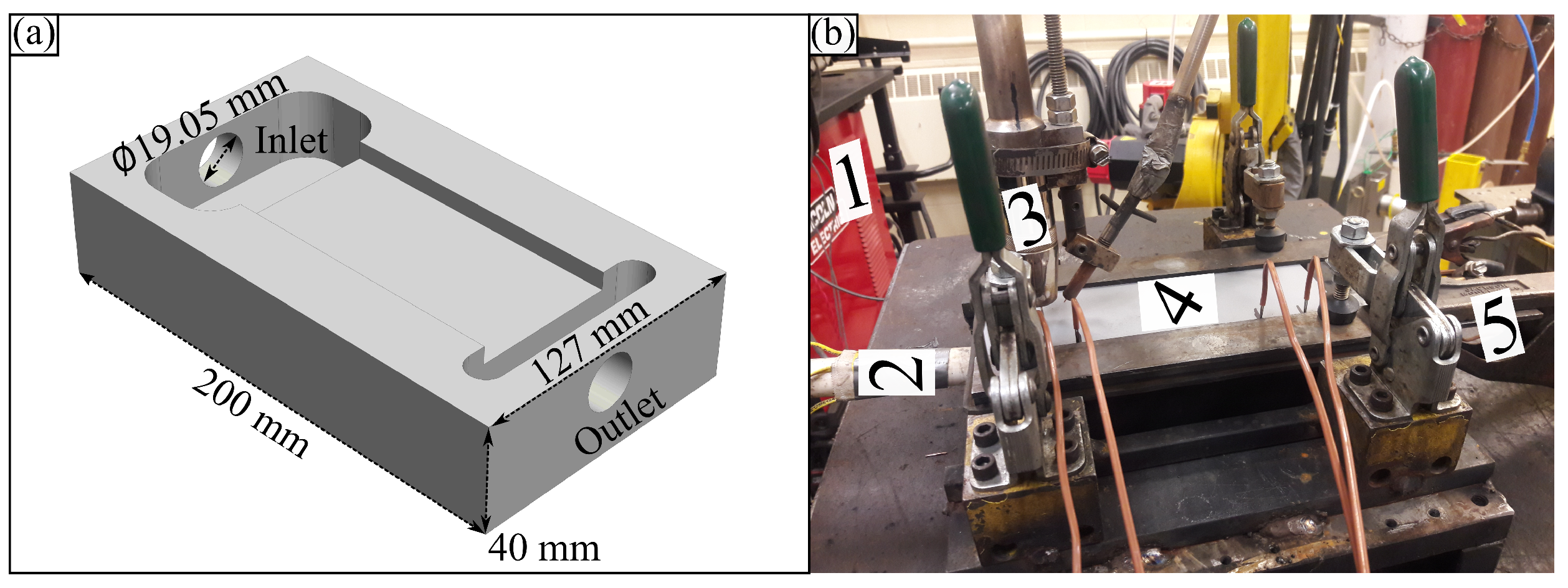
Figure 2.
A schematic of a cross-section of a weld bead. This figure is only a schematic representation of a general welding profile, and it was not designed to mirror actual profiles as shown in Figure 3.
Figure 2.
A schematic of a cross-section of a weld bead. This figure is only a schematic representation of a general welding profile, and it was not designed to mirror actual profiles as shown in Figure 3.
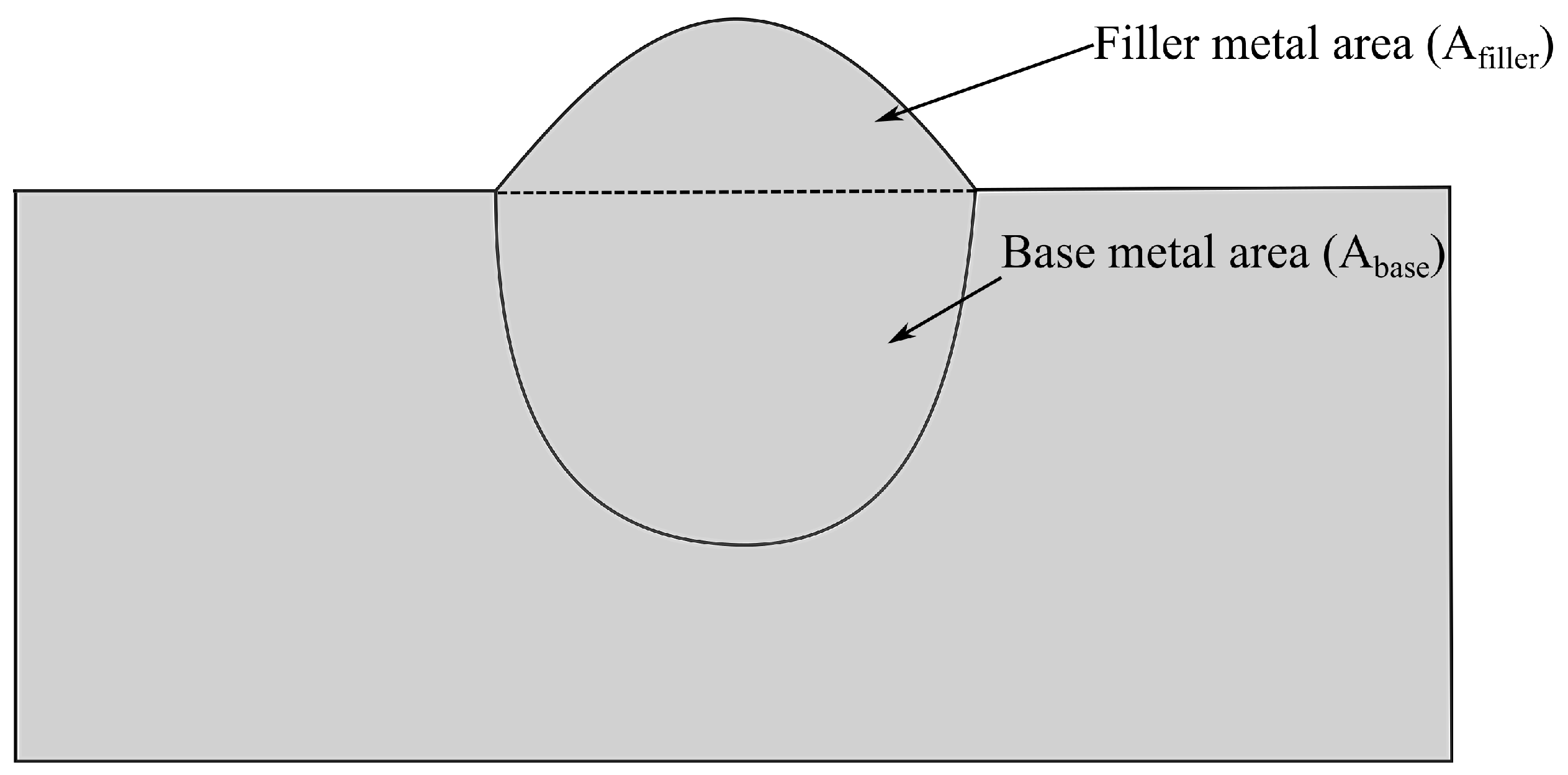
Figure 3.
Cross-sections of the welds for different metal transfer regimes: (a) short-circuit, (b) globular, and (c) spray. Thin plate (6 mm) and thick plate (9.5 mm), and for both 5 L/min was the calorimeter flow rate employed.
Figure 3.
Cross-sections of the welds for different metal transfer regimes: (a) short-circuit, (b) globular, and (c) spray. Thin plate (6 mm) and thick plate (9.5 mm), and for both 5 L/min was the calorimeter flow rate employed.
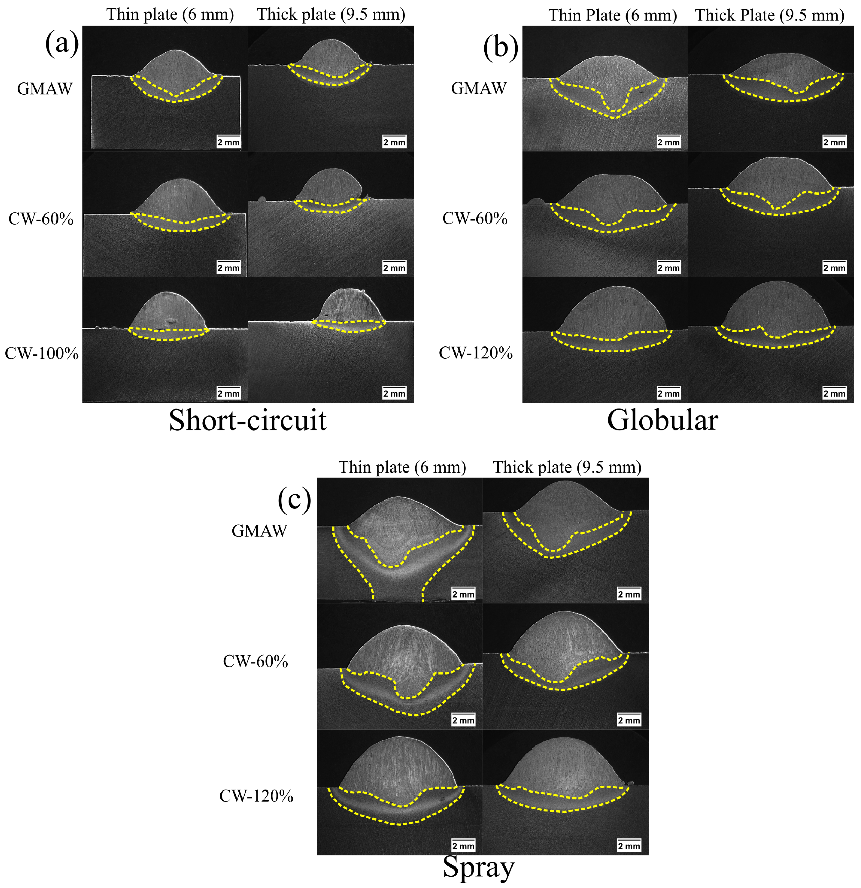
Figure 4.
Melting efficiency in short-circuit transfer mode: (a) standard GMAW; (b) CW-GMAW-60%; and (c) CW-GMAW-10%. In this figure, the conditions were thin plate (6 mm) and thick plate (9.5 mm), and for both, 5 L/min was the calorimeter flow rate employed. The error bars represent 95% confidence intervals.

Figure 5.
Melting efficiency in globular transfer mode: (a) standard GMAW; (b) CW-GMAW-60%; and (c) CW-GMAW-120%. In this figure, the conditions were thin plate (6 mm) and thick plate (9.5 mm), and for both, 5 L/min was the calorimeter flow rate employed. The error bars represent 95% confidence intervals.

Figure 6.
Melting efficiency in spray transfer mode: (a) standard GMAW; (b) CW-GMAW-60%; and (c) CW-GMAW-120%. In this figure, the conditions were thin plate (6 mm) and thick plate (9.5 mm), and for both, 5 L/min was the calorimeter flow rate employed. The error bars represent 95% confidence intervals.

Figure 7.
(a) Rykalin and (b) Christensen numbers for different cold wire feed rates for the short-circuit metal transfer regime. The error bars are 95% confidence intervals.
Figure 7.
(a) Rykalin and (b) Christensen numbers for different cold wire feed rates for the short-circuit metal transfer regime. The error bars are 95% confidence intervals.
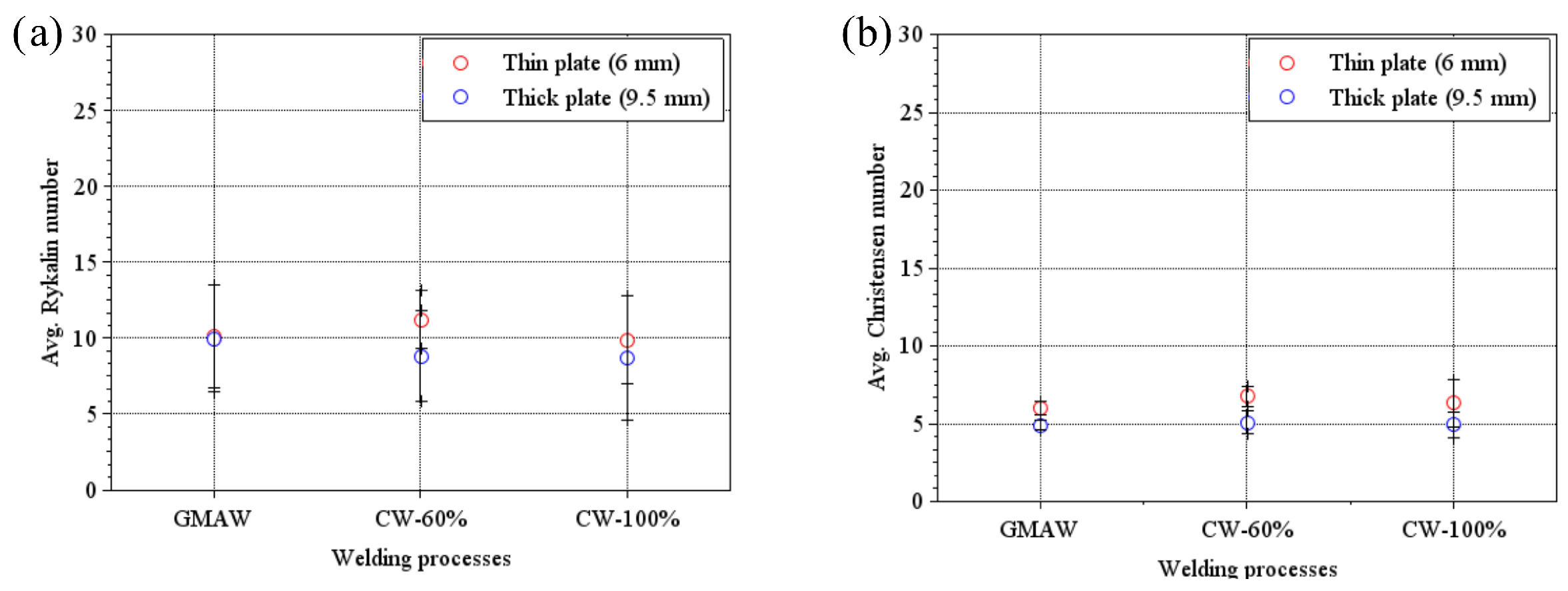
Figure 8.
(a) Rykalin and (b) Christensen numbers for different cold wire feed rates for the globular metal transfer regime. The error bars are 95% confidence intervals.
Figure 8.
(a) Rykalin and (b) Christensen numbers for different cold wire feed rates for the globular metal transfer regime. The error bars are 95% confidence intervals.
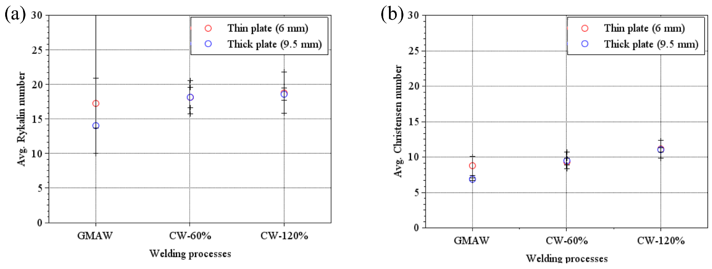
Figure 9.
(a) Rykalin and (b) Christensen numbers for different cold wire feed rates for the spray metal transfer regime. The error bars are 95% confidence intervals.
Figure 9.
(a) Rykalin and (b) Christensen numbers for different cold wire feed rates for the spray metal transfer regime. The error bars are 95% confidence intervals.
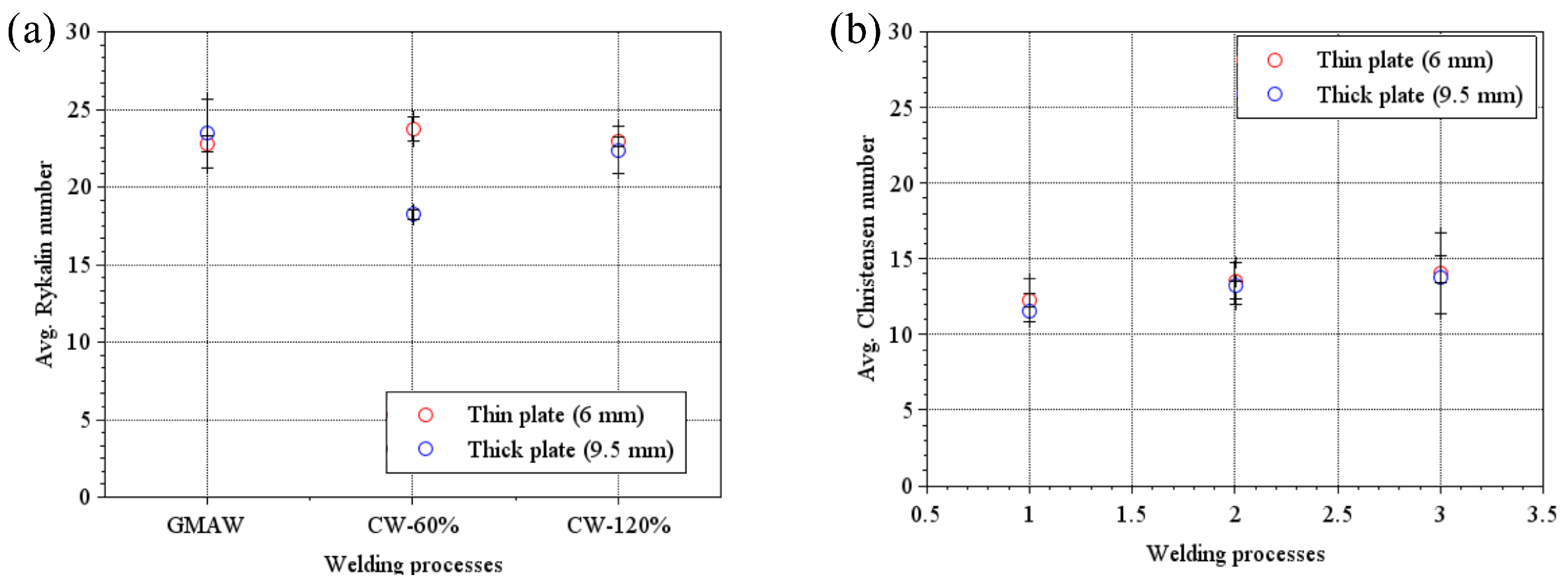
Figure 10.
A comparison between the melting efficiencies calculated by the two approaches discussed: (a) short-circuit, (b) globular, and (c) spray.
Figure 10.
A comparison between the melting efficiencies calculated by the two approaches discussed: (a) short-circuit, (b) globular, and (c) spray.
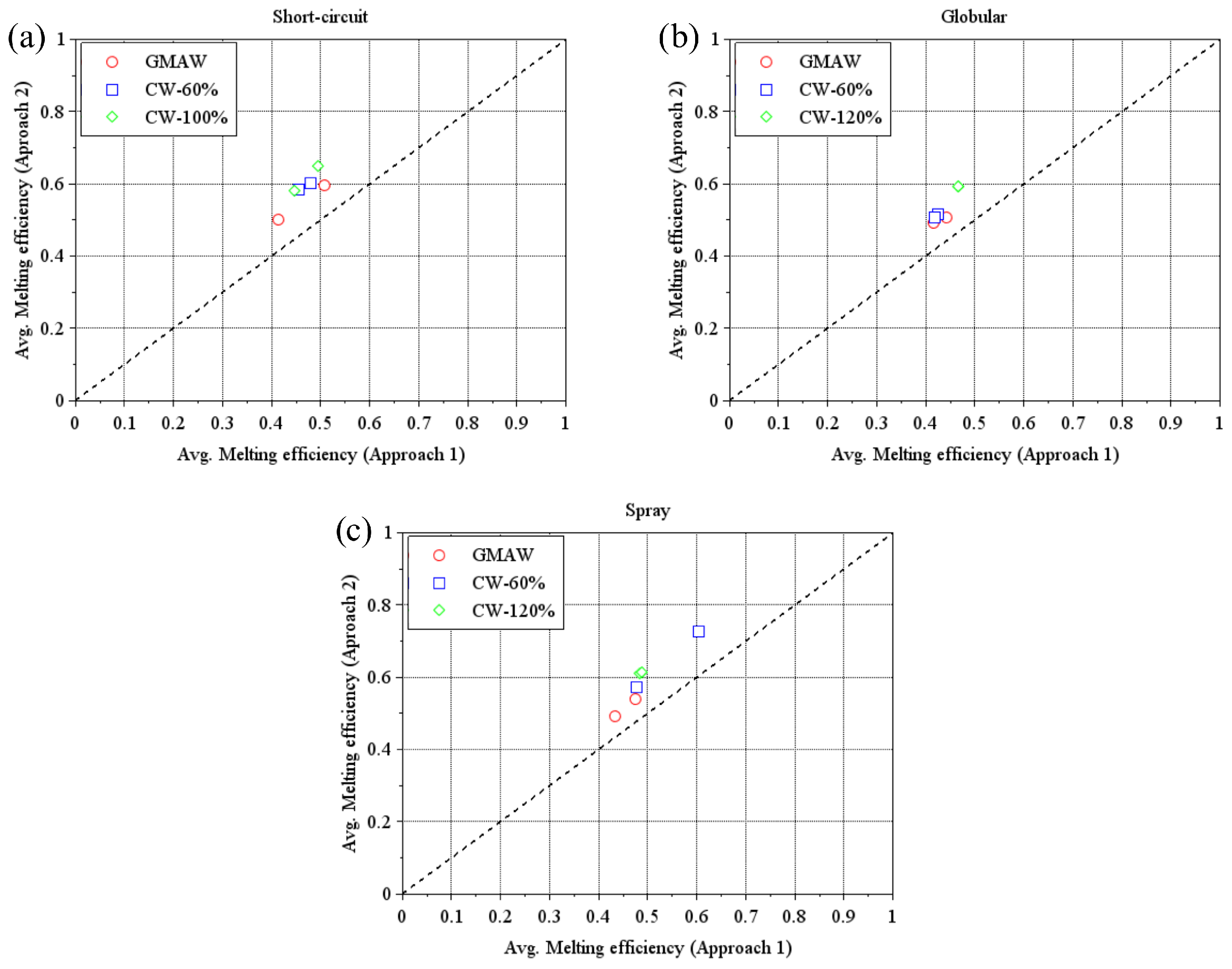
Figure 11.
Christensen versus Rykalin number for thin and thick plates: (a) no cold wire feed rates (GMAW), (b) intermediate cold wire feed rates (60%), and (c) high cold wire feed rates (100% and 120%). The values that assess the quality of the regression are shown in Table 5.
Figure 11.
Christensen versus Rykalin number for thin and thick plates: (a) no cold wire feed rates (GMAW), (b) intermediate cold wire feed rates (60%), and (c) high cold wire feed rates (100% and 120%). The values that assess the quality of the regression are shown in Table 5.

Table 1.
Welding parameters for the experiments reported in this work.
| Short-Circuit Transfer Mode | |||||
|---|---|---|---|---|---|
| Process | WFS (in/min) [m/min] | Voltage (V) | Travel Speed (in/min) [cm/min] | CTWD (mm) | Cold Wire Mass Feed Rate (%) [in/min] {m/min} |
| GMAW | 250 [6.35] | 20 | 25 [63.5] | 17 | - |
| CW-GMAW-60% | 250 | 20 | 25 | 17 | 60 [267] {6.7} |
| CW-GMAW-100% | 250 | 20 | 25 | 17 | 100 [444] {11.3} |
| Globular Transfer Mode | |||||
| GMAW | 280 [7.11] | 28 | 25 | 17 | - |
| CW-GMAW-60% | 280 | 28 | 25 | 17 | 60 [299] {7.6} |
| CW-GMAW-120% | 280 | 28 | 25 | 17 | 120 [597] {15.2} |
| Spray Transfer Mode | |||||
| GMAW | 350 [8.89] | 30 | 25 | 17 | - |
| CW-GMAW-60% | 350 | 30 | 25 | 17 | 60 [373] {9.5} |
| CW-GMAW-120% | 350 | 30 | 25 | 17 | 120 [747] {18.9} |
Table 2.
Calorimeter test set-up parameters.
| Bead Metal Condition | Flow Rate (L/min) | Plate Thickness (mm) [in] |
|---|---|---|
| Thin plate (6 mm) | 5 | 6.35 |
| Thick plate (9.5 mm) | 5 | 9.53 |
Table 3.
The average electrical values measured during the experimental conditions reported in this work.
Table 3.
The average electrical values measured during the experimental conditions reported in this work.
| Short-Circuit Transfer Mode | ||||
|---|---|---|---|---|
| Process | Avg. Current (V) | Avg. Voltage (A) | Avg. Power (W) | Nominal Heat Input (J/mm) |
| GMAW | 213 | 20 | 4465 | 422 |
| CW-60% | 218 | 20 | 4488 | 424 |
| CW-100% | 220 | 20 | 4560 | 431 |
| Globular Transfer Mode | ||||
| GMAW | 250 | 29 | 7186 | 679 |
| CW-60% | 256 | 28 | 7282 | 688 |
| CW-120% | 256 | 28 | 7179 | 678 |
| Spray Transfer Mode | ||||
| GMAW | 299 | 30 | 9032 | 853 |
| CW-60% | 297 | 30 | 8905 | 841 |
| CW-120% | 302 | 30 | 9082 | 858 |
Table 4.
Heat transfer modes for the three welding regimes, calculated from the relative plate thickness using the threshold value of 0.75 to avoid the intermediate heat transfer regime. Thin plate (6 mm) and thick plate (9.5 mm), and for both, 5 L/min was the calorimeter flow rate employed. The values between parenthesis correspond to the actual values of relative plate thickness .
| Short-Circuit Regime | Globular Regime | Spray Regime | |||
|---|---|---|---|---|---|
| Base Metal Condition/ Welding Process | Heat Transfer Regime | Base Metal Condition/ Welding Process | Heat Transfer Regime | Base Metal Condition/ Welding Process | Heat Transfer Regime |
| Thin plate/GMAW | 3D (0.85) | Thin plate/GMAW | 2D (0.65) | Thin plate/GMAW | 2D (0.62) |
| Thick plate/GMAW | 3D (1.28) | Thick plate/GMAW | 3D (1.08) | Thick plate/GMAW | 3D (0.91) |
| Thin plate/CW-60% | 3D (0.80) | Thin plate/CW-60% | 2D (0.63) | Thin plate/CW-60% | 2D (0.60) |
| Thick plate/CW-60% | 3D (1.33) | Thick plate/CW-60% | 3D (0.93) | Thick plate/CW-60% | 3D (1.04) |
| Thin plate/CW-100% | 3D (0.85) | Thin plate/CW-120% | 2D (0.62) | Thin plate/CW-120% | 2D (0.61) |
| Thick plate/CW-100% | 3D (1.37) | Thick plate/CW-120% | 3D (0.92) | Thick plate/CW-120% | 3D (0.94) |
Table 5.
Pearson’s coefficient, , and Adj. coefficient for all the conditions. The values of and Adj. presented in this table refer to the trend lines presented in Figure 11.
Table 5.
Pearson’s coefficient, , and Adj. coefficient for all the conditions. The values of and Adj. presented in this table refer to the trend lines presented in Figure 11.
| Process | Plate Thickness (mm) | CW Feed Rate (%) | Pearson’s Coefficient | Adj. Coefficient | |
|---|---|---|---|---|---|
| GMAW | 6 (Thin) | None (0%) | 0.985 | 0.969 | 0.939 |
| GMAW | 9.5 (Thick) | 0.999 | 0.999 | 0.999 | |
| CW-GMAW | 6 | Intermediate (60%) | 0.981 | 0.962 | 0.924 |
| CW-GMAW | 9.5 | 0.864 | 0.748 | 0.495 | |
| CW-GMAW | 6 | High (100% and 120%) | 0.998 | 0.995 | 0.991 |
| CW-GMAW | 9.5 | 0.999 | 0.999 | 0.998 |
Disclaimer/Publisher’s Note: The statements, opinions and data contained in all publications are solely those of the individual author(s) and contributor(s) and not of MDPI and/or the editor(s). MDPI and/or the editor(s) disclaim responsibility for any injury to people or property resulting from any ideas, methods, instructions or products referred to in the content. |
© 2024 by the authors. Licensee MDPI, Basel, Switzerland. This article is an open access article distributed under the terms and conditions of the Creative Commons Attribution (CC BY) license (https://creativecommons.org/licenses/by/4.0/).
Share and Cite
MDPI and ACS Style
Ribeiro, R.A.; Assunção, P.D.C.; Gerlich, A.P. Evaluation of Melting Efficiency in Cold Wire Gas Metal Arc Welding Using 1020 Steel as Substrate. Metals 2024, 14, 484. https://doi.org/10.3390/met14040484
AMA Style
Ribeiro RA, Assunção PDC, Gerlich AP. Evaluation of Melting Efficiency in Cold Wire Gas Metal Arc Welding Using 1020 Steel as Substrate. Metals. 2024; 14(4):484. https://doi.org/10.3390/met14040484
Chicago/Turabian StyleRibeiro, R. A., P. D. C. Assunção, and A. P. Gerlich. 2024. "Evaluation of Melting Efficiency in Cold Wire Gas Metal Arc Welding Using 1020 Steel as Substrate" Metals 14, no. 4: 484. https://doi.org/10.3390/met14040484
Note that from the first issue of 2016, this journal uses article numbers instead of page numbers. See further details here.