Anisotropic Hardening Behaviour and Springback of Advanced High-Strength Steels
by
 ,
,
Jaebong Jung
1 ,
,
Sungwook Jun
1,
Hyun-Seok Lee
2,
Byung-Min Kim
1,
Myoung-Gyu Lee
3 and
Ji Hoon Kim
1,* 1
School of Mechanical Engineering, Pusan National University, Busan 46241, Korea
2
NARA Mold & Die Co., Ltd., Changwon 51555, Korea
3
Department of Materials Science and Engineering, Korea University, Seoul 02841, Korea
*
Author to whom correspondence should be addressed.
Metals 2017, 7(11), 480; https://doi.org/10.3390/met7110480
Submission received: 26 September 2017
/
Revised: 6 October 2017
/
Accepted: 12 October 2017
/
Published: 6 November 2017
(This article belongs to the Special Issue Advances in Plastic Forming of Metals)
Abstract
:Advanced high-strength steels (AHSSs) exhibit large, and sometimes anisotropic, springback recovery after forming. Accurate description of the anisotropic elasto-plastic behaviour of sheet metals is critical for predicting their anisotropic springback behaviour. For some materials, the initial anisotropy is maintained while hardening progresses. However, for other materials, anisotropy changes with hardening. In this work, to account for the evolution of anisotropy of a dual-phase steel, an elastoplastic material constitutive model is developed. In particular, the combined isotropic–kinematic hardening model was modified. Tensile loading–unloading, uniaxial and biaxial tension, and tension–compression tests were conducted along the rolling, diagonal, and transverse directions to measure the anisotropic properties, and the parameters of the proposed constitutive model were determined. For validation, the proposed model was applied to a U-bending process, and the measured springback angles were compared to the predicted ones.
1. Introduction
Weight reduction, in order to improve fuel efficiency and meet CO2 regulations for addressing global warming while maintaining safety regulations, is an important issue in automotive manufacturing [1,2]. In this work, we investigate the application of advanced high-strength steels (AHSSs), with good strength and formability, in automotive parts. The demand for automotive parts made of AHSSs is based on their excellent impact resistance, which is an asset for the reinforcement of the car body structure, and which depends on their high strength [3,4,5,6,7]. However, along with their high strength and low thickness, the AHSSs exhibit anisotropic properties and large springback recovery after forming [8,9]. The higher their strength and the thinner the sheet metals, the greater the tendency for anisotropy and springback to occur [10,11]. For some metals, the anisotropy of a material follows a tendency determined at the initial yielding, which does not change as hardening progresses. However, in several cases of materials in which the anisotropic tendency changes according to the hardening progress, there is a restriction to express the phenomenon of anisotropic springback problem with a yield function and the conventional hardening rules. Therefore, the accurate description of the anisotropic elasto-plastic behaviour of sheet metals is critical for predicting their anisotropic springback behaviour.
To predict springback accurately, it is important to use sophisticated elastic material models [12,13,14,15]. A constant elastic modulus is widely used, but it is not suitable for representing anisotropic and nonlinear unloading behaviour. Lems [16] investigated a change in the elastic modulus following the plastic strain at low temperature and its recovery. Morestin and Boivin [17] proved that the variation in the elastic modulus following a plastic strain allows better numerical analysis of the elasto-plastic phenomenon in the case of the springback problem. Steels, for example, have a reduction of up to 20–30% of their initial elastic modulus (), while for aluminium alloys, in general, the reduction is 20%. The chord modulus model [18] represents a changing elastic modulus behaviour according to the hardening progress by reducing the elastic modulus with the increase in equivalent plastic strain. This model can improve the accuracy in springback prediction, because it is effective in expressing the reduction phenomenon and is computationally efficient. Its disadvantage is that a nonlinear stress–strain response cannot be captured. As a result, the stress–strain description is accurate only when fully loaded. In the quasi-plastic-elastic (QPE) model proposed by Sun and Wagoner [19], the elastic modulus is maintained as the initial value until reaching a certain level of stress based on the QPE rules, and then, the elastic modulus, according to the strain amount, is nonlinearly reduced until reaching the next plastic behaviour.
The springback predictions are also sensitive to yield functions for materials having highly anisotropic properties [20,21,22]. The Yld2000-2d yield function [23] is widely used in sheet metal forming simulations. The Bauschinger effect is usually described by introducing back stresses, as in the Armstrong-Frederick hardening rule [24]. To account for the nonlinear hardening and changing anisotropic tendency, variable parameters and tensors have been introduced into the back stress evolution rule [25,26]. Recently, the homogeneous yield function-based anisotropic hardening (HAH) model [27] was proposed, wherein the plastic behaviour of a metallic material subjected to multiple or continuous strain path changes is described using a collapse of the yield function. A fluctuating term of the HAH model, along with phenomenological or dislocation density-based hardening equations, can depict an anisotropic hardening according to the change in various strain paths [28,29,30].
The dual-phase (DP) steels studied in this work are generally subjected to intercritical annealing of cold rolled strips followed by quenching and as a result, they have a microstructure consisting of a ferritic matrix and a martensitic islands [31]. The quenching converts the ferrite-mixed austenite phase to martensite, leading to a ferrite–martensite two-phase system. The complex microstructure of DP steels may cause complicated behaviour upon changes in loading paths.
In this work, to account for the evolution of anisotropy in a DP steel, an elastoplastic material constitutive model is developed. In particular, the combined isotropic–kinematic hardening model was modified. Tensile loading–unloading, uniaxial and biaxial tension, and tension–compression tests were conducted along the rolling (RD), diagonal (DD), and transverse (TD) directions to measure the anisotropic properties, and the parameters of the proposed constitutive model were determined. For validation, the proposed model was applied to a U-bending process, and the measured and predicted springback angles were compared.
2. Constitutive Equations
2.1. Elasticity
A stress-strain relationship of a material under a non-yielding condition may be expressed by the generalised Hooke’s law [32]:
where is elastic strain, is Cauchy stress, and C is the stiffness matrix. Under the plane stress condition and with the isotropic elasticity, Equation (1) may be rewritten in the matrix form as [32]:
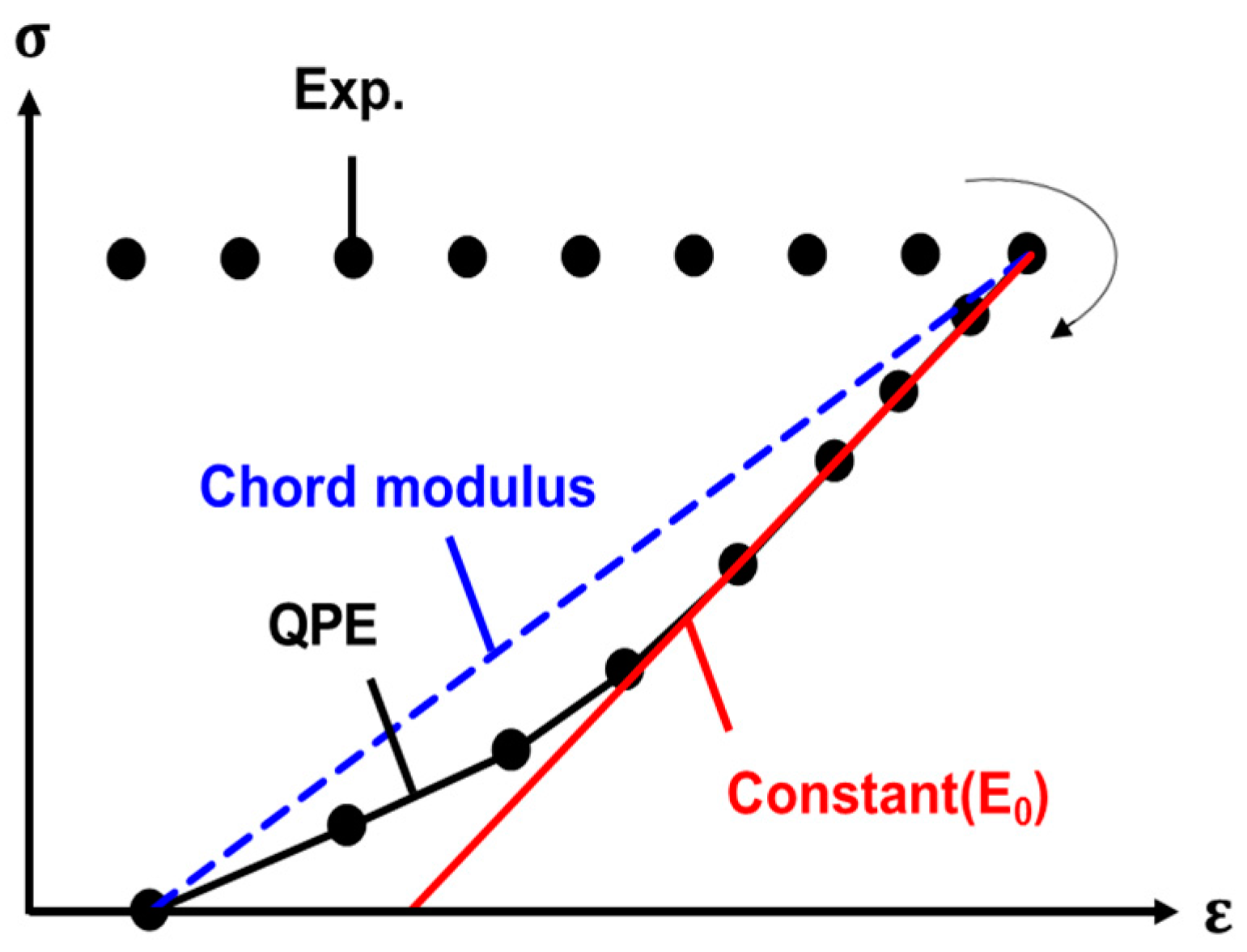
where is the Young’s modulus, is the shear modulus, and is the Poisson’s ratio. The Young’s modulus can be express by various elastic material models, as shown in Figure 1. The constant modulus model underestimates the elastic recovery, whereas the chord modulus model overestimates it. The QPE model [19] can depict the elastic unloading behaviour by introducing a QPE function and its nonlinear evolution. In the QPE model, the elastic modulus is given by:
where is the initial elastic modulus and and are material parameters determined by loading–unloading tests. and are, respectively, increment of total strain and plastic strain. In the QPE model, the QPE surface is defined where the constant elastic modulus is used:
where , are the QPE function, its center, and the size of the QPE function, respectively. The size of the QPE function is assumed constant in this work. In the QPE mode, the stress is located outside of and inside of f.
2.2. Yield Criterion
The Yld2000-2d yield function [23], f, composed of two functions, and , was used to account for the anisotropic yielding
where is the stress, is the effective stress, and m is the yield function exponent. The details of the yield function are given in Appendix A.
2.3. Hardening Law
The back stress, , is introduced to account for the Bauschinger effect in the Armstrong-Frederick hardening model [24]:
where the yield function size of the isotropic hardening law of Voce type [33], , is given by:
where , , and are material parameters. The yield function is an m-th order homogeneous function, whose size is decided by the equivalent plastic strain . Yielding occurs when the yield function equals its size. In the Armstrong–Frederick hardening model, the increment in the back stress is composed of two terms:
where and are material parameters. The second term of the furthest right side of Equation (8) is called a recall term, which is introduced by expressing the transient behaviour of the gradually disappearing memory of the material when subjected to a rapid change in the stress. The hardening rate increases if of the first term increases and non-linear hardening appears when increases under a reverse loading condition.
Chung et al. [25] proposed a back stress evolution rule, where and are functions of the equivalent plastic strain, for expressing general hardening behaviour. In this paper, and were expressed as:
where , , , , , and are material parameters.
To account for the anisotropic evolution of back stress [26], the back stress evolution rule was modified as:
where and are 3 × 3 diagonal tensors given by:
This model is denoted as ‘the hardening model with anisotropic evolution’. If the back stress evolves isotropically (), it is denoted as ‘the hardening model with the isotropic evolution’.
3. Experiments
A dual-phase steel with tensile strength of 980 MPa and thickness of 1.1 mm (DP980) was used for the mechanical and U-bending tests. The uniaxial tension, uniaxial tensile loading–unloading, and biaxial tension tests were conducted to determine the material parameters of the QPE model and the Yld2000-2d yield function. The hardening parameters of the isotropic and anisotropic evolution models were obtained from the tension–compression tests. The U-bending test was conducted to evaluate the effect of the anisotropic evolution on springback.
3.1. Uniaxial Tensile and Loading–Unloading Tests
The uniaxial tensile and loading–unloading tests were carried out using a universal testing machine. The ASTM E8 standard size specimens were manufactured by wire electrodischarge machining. The effect of the coupon manufacturing methods on tensile properties were discussed elsewhere [34]. The uniaxial tensile tests were conducted for the RD, DD, and TD, as shown in Figure 2a. The loading–unloading tests were conducted for pre-strains of 3, 5, and 7% in the RD, as shown in Figure 2b. The material properties were obtained following the standard test methods ASTM E8 (Standard Test Method for Tension Testing of Metallic Materials) and E517 (Standard Test Method for Plastic Strain Ratio r for Sheet Metal), as listed in Table 1.
The parameters of the QPE model were derived from the loading–unloading data, as listed in Table 2.
3.2. Biaxial Tensile Test
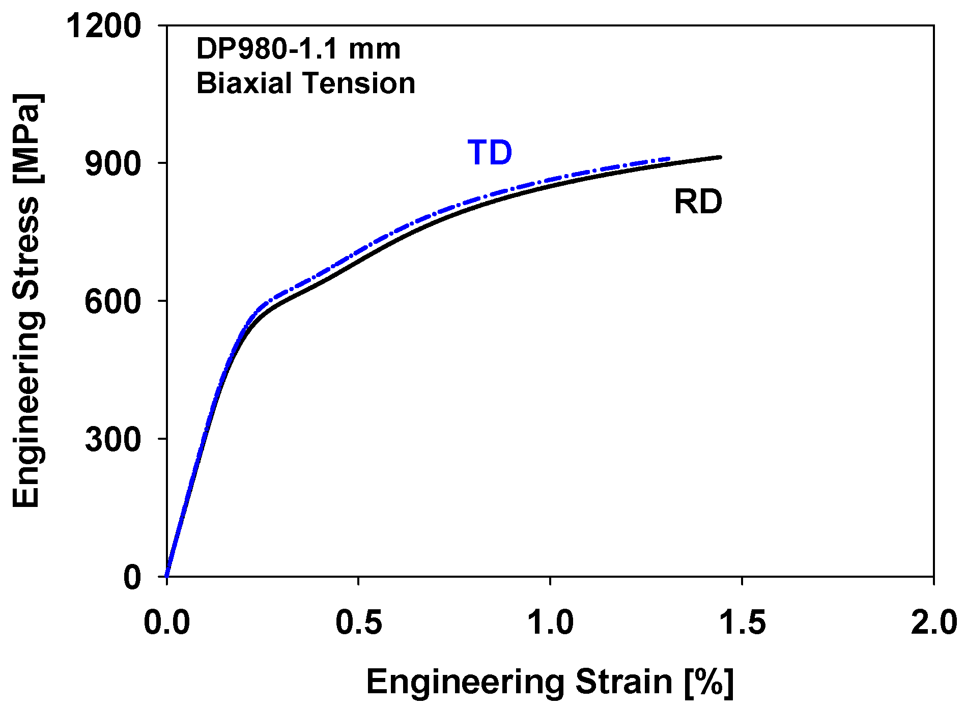
The balanced biaxial (BB) tensile test was carried out using a biaxial tensile tester [35] with a cruciform specimen, as shown in Figure 3. A constant loading rate of 9.8 kN/min was used. The plastic strain ratio in balanced biaxial tension was obtained. The results of the balanced biaxial tension are shown in Figure 4 and listed in Table 3.
3.3. Tension-Compression Test
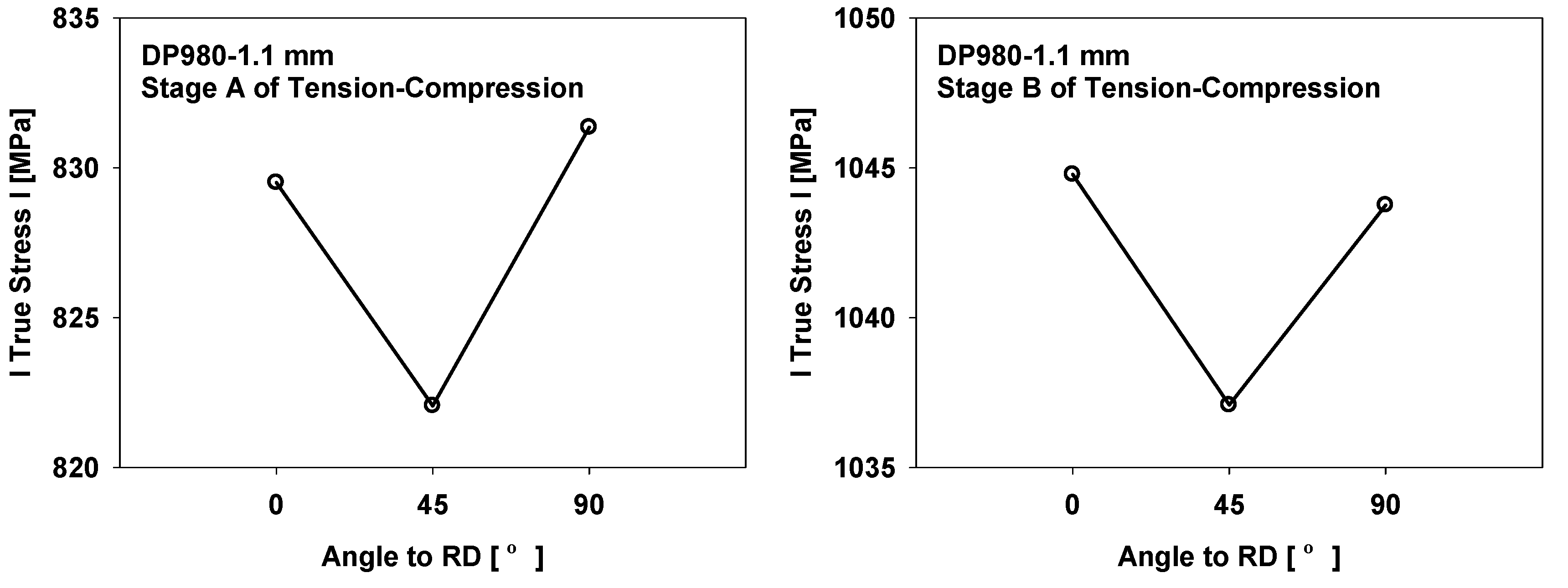
In order to investigate the anisotropic evolution of hardening, tension–compression tests were carried out in the three material directions using a tension–compression tester, as shown in Figure 6. In the tension-compression test, the sheet specimen is placed between the comb-shaped anti-buckling fixtures. Buckling of the sheet metals, which may occur during compression, is suppressed by the hydraulic force acting perpendicular to the sheet plane through the comb-shaped fixtures. Details of the tension-compression test can be found elsewhere [36]. In the tension-compression tests, the tension by a strain of 7% was followed by the compression to a strain of −7%. The true stress-accumulated plastic strain curves can be divided into three stages, as shown in Figure 7. In stage A, where hardening hardly progresses, the anisotropic tendency of yielding matches the initial yield strength trend in Figure 5a. The curves of RD and TD become similar in stage B, and the flow stress of RD becomes larger than that of TD in stage C where the initial anisotropic tendency is reversed. The change in anisotropic tendency is illustrated in Figure 8.
The hardening model parameters were obtained from the tension–compression data by optimisation using the fminsearch function of the MATLAB program, as listed in Table 5. The MATLAB function finds parameters that minimise the error function value using the Nelder–Mead method [37]. After calculating a residual by performing a finite element (FE) analysis using an estimated value, the fminsearch function calculates the updated parameter values and repeats the FE analysis. This process is repeated until no further reduction in residual is achieved. In the case of the hardening model with isotropic hardening, it was optimised only for the rolling direction data.
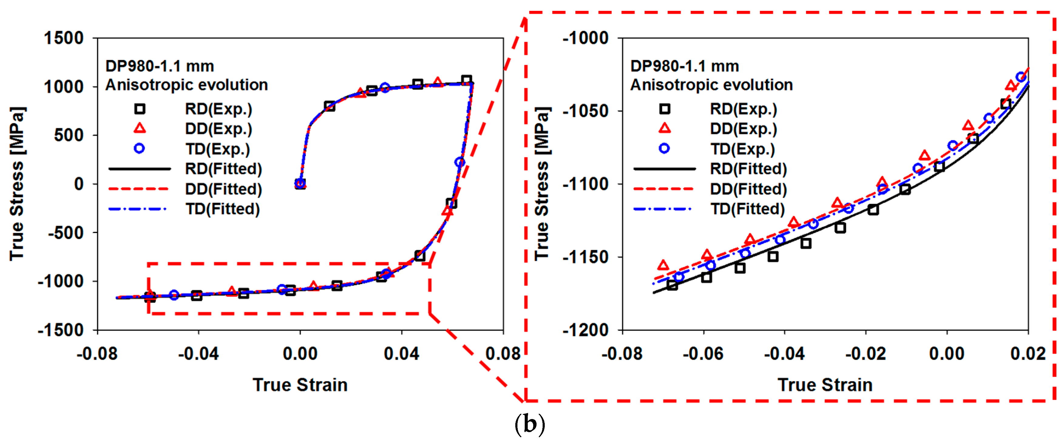
In Figure 9, the tension-compression curves in the three material directions were compared. In the case of the isotropic evolution, it follows the initial trend of anisotropy determined by the yield function. However, in the case of the anisotropic evolution, the anisotropic tendency is changed during reverse loading. The errors of fit of the tension–compression curves predicted by the isotropic and anisotropic evolution models are compared in Figure 10. The error of fit in the RD value is similar because the parameters of the isotropic model were obtained from the RD data. However, the errors in the DD and TD are smaller for the anisotropic models.
4. Application
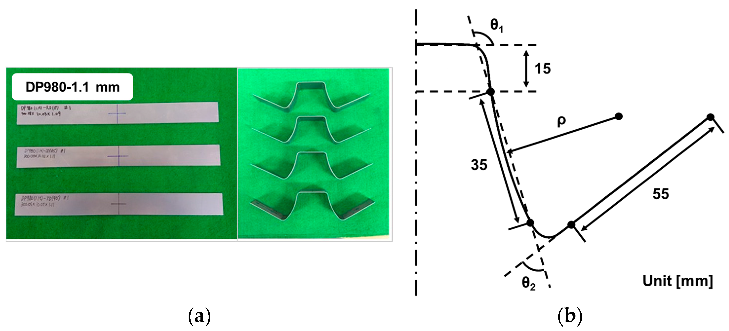
U-bending tests were conducted using specimens with size of 300 30 1.1 mm3 for the three material directions. The experiments were performed using a servo-press. The dimensions of the test are shown in Figure 11a. The holding force was linearly increased from 5.65 kN to 7.92 kN from the beginning to the end of the punch stroke. The specimens before and after forming and springback are shown in Figure 12a.
Simulations of the U-bending process were carried out using the commercial finite element software Abaqus/Standard, as shown in Figure 11b. Four-node shell elements with reduced integration (S4R) were used with an element size of 0.5 mm. The number of integration points through the thickness was seven. The coefficient of friction was assumed as 0.12. The deformation of the tools may affect the U-bending test results significantly [38]. However, for simplicity, the punch, die, and holder were assumed as rigid bodies in this work.
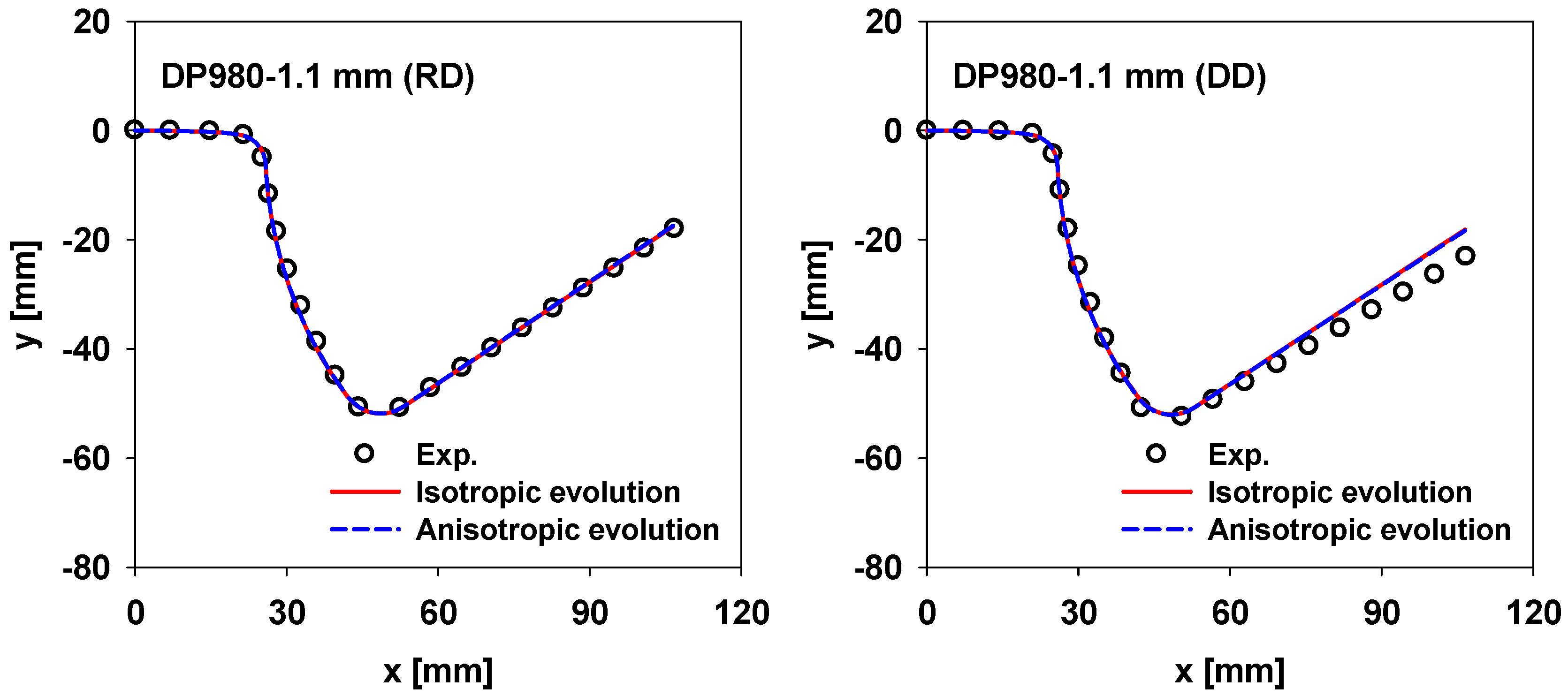
The measured and calculated shapes of the specimens after springback are compared for the three material directions in Figure 13. The predicted shapes showed good agreements with the measurements in RD, while there are some differences in DD and TD. The predictions with the isotropic and anisotropic evolution showed little differences for RD because the material parameters of the isotropic evolution model were fitted for RD. However, the predictions with the isotropic and anisotropic evolution showed differences in TD, although the amount of the difference is small.
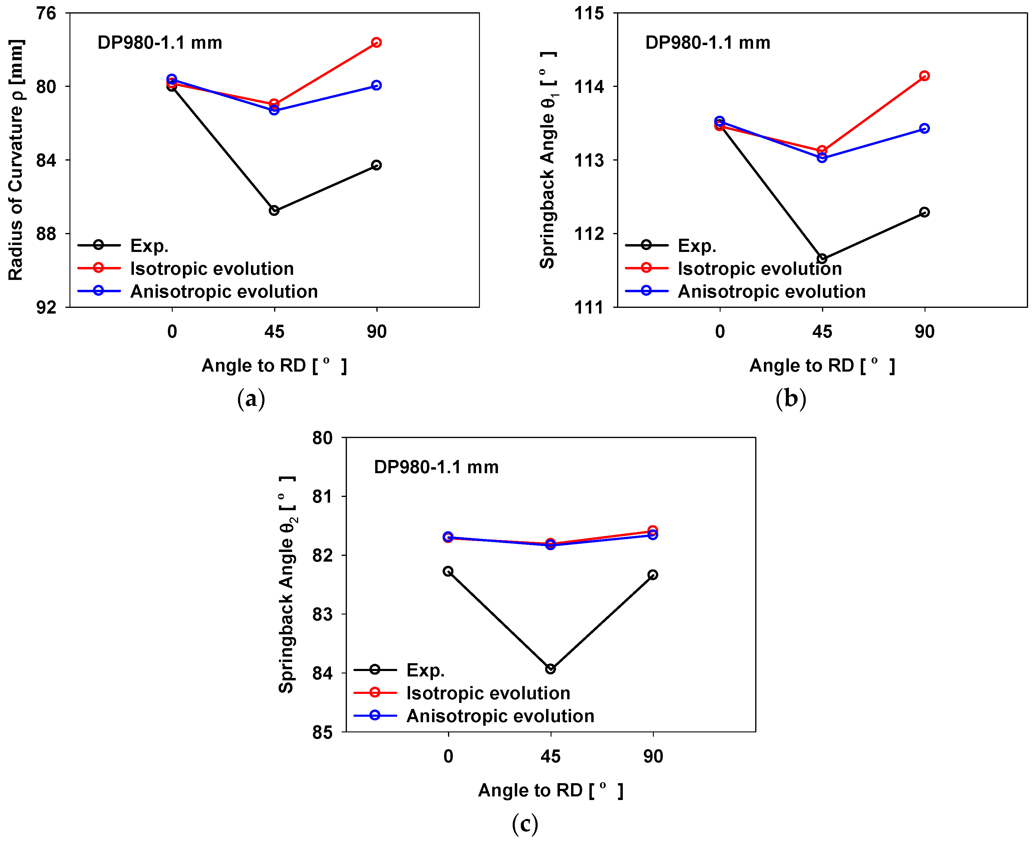
In order to evaluate the springback quantitatively, three measures of springback (, , and ), defined in Figure 12b, were taken from the specimen geometry, as shown in Figure 14. The predictions with the isotropic and anisotropic evolution showed little differences in the U-bending shape of the RD and DD specimens. For the TD specimens, the predictions with the anisotropic evolution showed better agreements with the measurements. This is because the anisotropic hardening evolution rule reduces the error when representing the stress-strain behaviour in directions other than RD. In the case of the isotropic evolution model, the initial yielding anisotropic tendency of the yield function is maintained in the springback result of U-bending. However, the initial anisotropic tendency was changed during deformation, as shown in Figure 8. In the case of the anisotropic evolution model, the evolving anisotropy tendency is represented, which is more similar to the measurements.
5. Conclusions
To account for the evolution of anisotropy of a dual-phase steel, an elastoplastic material constitutive model is developed by modifying the combined isotropic-kinematic hardening model. The tensile loading–unloading, uniaxial and biaxial tension, and tension–compression tests were conducted along the rolling, diagonal, and transverse directions to measure the anisotropic properties, and the parameters of the proposed constitutive model were determined. For validation, the proposed model was applied to a U-bending process, and the measured and predicted springback angles were compared. The following conclusions were drawn:
- The dual-phase steel studied in this work exhibited a change in the anisotropic properties during deformation.
- The hardening model with the anisotropic evolution successfully captured the evolution of the angular variation of anisotropic properties.
- Using the hardening model with anisotropic evolution, it was possible to accurately predict the springback in different directions.
Acknowledgments
This work was supported by the Small and Medium Business Administration of Korea (SMBA) grant funded by the Korean government (MOTIE) (No. S2315965) and the National Research Foundation of Korea (NRF) grant funded by the Korean government (MSIP) (No. 2012R1A5A1048294).
Author Contributions
Jaebong Jung and Ji Hoon Kim conceived and designed the experiments; Jaebong Jung and Sungwook Jun performed the experiments; Jaebong Jung, Sungwook Jun, Ji Hoon Kim, Byoung Min Kim, and Myoung-Gyu Lee analysed the data; Hyun-Seok Lee contributed with materials/analysis tools; Jaebong Jung and Ji Hoon Kim wrote the paper.
Conflicts of Interest
The authors declare no conflict of interest.
Appendix A
The Yld2000-2d yield function [6] has eight parameters () that require eight mechanical properties (, , , , , , , ). The m value is suggested as six for BCC and eight for FCC metal. In Equation (4), the yield function is given by a combination of two functions:
where the and are principal values of the tensor and , respectively, which are expressed by the product of the anisotropic components ( or ) and stress components ( or ).
References
- Keeler, S.; Kimchi, M. Advanced High-Strength Steels Application Guidelines Version 5.0; WorldAutoSteel: Middletown, OH, USA, 2014. [Google Scholar]
- Cheah, L.W. Cars on a Diet: The Material and Energy Impacts of Passenger Vehicle Weight Reduction in the U.S. Ph.D. Thesis, Massachusetts Institute of Technology, Cambridge, MA, USA, September 2010. [Google Scholar]
- Amigo, F.J.; Camacho, A.M. Reduction of induced central damage in cold extrusion of dual-phase steel DP980 using double-pass dies. Metals 2017, 7, 335. [Google Scholar] [CrossRef]
- Xue, X.; Pereira, A.B.; Amorim, J.; Liao, J. Effects of pulsed Nd: YAG laser welding parameters on penetration and microstructure characterization of a DP1000 steel butt joint. Metals 2017, 7, 292. [Google Scholar] [CrossRef]
- Evin, E.; Tomas, M. The influence of laser welding on the mechanical properties of dual phase and TRIP steels. Metals 2017, 7, 239. [Google Scholar] [CrossRef]
- Moeini, G.; Ramazani, A.; Myslicki, S.; Sundararaghavan, V.; Konke, C. Low cycle fatigue behaviour of DP steels: Micromechanical modelling vs. validation. Metals 2017, 7, 265. [Google Scholar] [CrossRef]
- Emre, H.E.; Kacar, R. Resistance spot weldability of galvanize coated and uncoated TRIP steels. Metals 2016, 6, 299. [Google Scholar] [CrossRef]
- Hassan, H.U.; Traphoner, H.; Guner, A.; Tekkaya, A.E. Accurate springback prediction in deep drawing using pre-strain based multiple cyclic stress-strain curves in finite element simulation. Int. J. Mech. Sci. 2016, 110, 229–241. [Google Scholar] [CrossRef]
- Lee, H.S.; Kim, J.H.; Kang, G.S.; Ko, D.C.; Kim, B.M. Development of seat side frame by sheet forming of DP980 with die compensation. Int. J. Precis. Eng. Manuf. 2017, 18, 115–120. [Google Scholar] [CrossRef]
- Abvabi, A.; Rolfe, B.; Hodgson, P.D.; Weiss, M. The influence of residual stress on a roll forming process. Int. J. Mech. Sci. 2015, 101–102, 124–136. [Google Scholar] [CrossRef]
- Liu, X.; Cao, J.; Chai, X.; Liu, J.; Zhao, R.; Kong, N. Investigation of forming parameters on springback for ultra high strength steel considering Young’s modulus variation in cold roll forming. J. Manuf. Process. 2017, 29, 289–297. [Google Scholar] [CrossRef]
- Lee, J.; Lee, J.Y.; Barlat, F.; Wagoner, R.H.; Chung, K.; Lee, M.G. Extension of quasi-plastic-elastic approach to incorporate complex plastic flow behaviour–application to springback of advanced high-strength steels. Int. J. Plast. 2013, 45, 140–159. [Google Scholar] [CrossRef]
- Chen, Z.; Bong, H.J.; Li, D.; Wagoner, R.H. The elastic-plastic transition of metals. Int. J. Plast. 2016, 83, 178–201. [Google Scholar] [CrossRef]
- Torkabadi, A.; Perdahcioglu, E.S.; Meinders, V.T.; Boogaard, V.D. On the nonlinear anelastic behaviour of AHSS. Int. J. Solids Struct. 2017, in press. [Google Scholar] [CrossRef]
- Lee, J.Y.; Lee, M.G.; Barlat, F.; Bae, G. Piecewise linear approximation of nonlinear unloading-reloading behaviours using a multi-surface approach. Int. J. Plast. 2017, 93, 112–136. [Google Scholar] [CrossRef]
- Lems, W. The change of Young’s modulus of copper and silver after deformation at low temperature and its recovery. Physica 1962, 28, 445–452. [Google Scholar] [CrossRef]
- Morestin, F.; Boivin, M. On the necessity of taking into account the variation in the Young modulus with plastic strain in elastic-plastic software. Nucl. Eng. Des. 1996, 162, 107–116. [Google Scholar] [CrossRef]
- Yoshida, F.; Uemori, T.; Fujiwara, K. Elastic-plastic behaviour of steel sheets under in-plane cyclic tension-compression at large strain. Int. J. Plast. 2002, 18, 633–659. [Google Scholar] [CrossRef]
- Sun, L.; Wagoner, R.H. Complex unloading behaviour: Nature of the deformation and its consistent constitutive representation. Int. J. Plast. 2011, 27, 1126–1144. [Google Scholar] [CrossRef]
- Cardoso, R.P.R.; Yoon, J.W. Stress integration method for a nonlinear kinematic/isotropic hardening model and its characterization based on polycrystal plasticity. Int. J. Plast. 2009, 25, 1684–1710. [Google Scholar] [CrossRef]
- Cao, J.; Lee, W.; Cheng, H.S.; Seniw, M.; Wang, H.P.; Chung, K. Experimental and numerical investigation of combined isotropic-kinematic hardening behaviour of sheet metals. Int. J. Plast. 2009, 25, 942–972. [Google Scholar] [CrossRef]
- Sumikawa, S.; Ishiwatari, A.; Hiramoto, J.; Urabe, T. Improvement of springback prediction accuracy using material model considering elastoplastic anisotropy and Bauschinger effect. J. Mater. Proc. Technol. 2016, 230, 1–7. [Google Scholar] [CrossRef]
- Barlat, F.; Brem, J.C.; Yoon, J.W.; Chung, K.; Dick, R.E.; Lege, D.J.; Pourboghrat, F.; Choi, S.H.; Chu, E. Plane stress yield function for aluminum alloy sheets-part 1: Theory. Int. J. Plast. 2003, 19, 1297–1319. [Google Scholar] [CrossRef]
- Frederick, C.O.; Armstrong, P.J. A mathematical representation of the multiaxial Bauschinger effect. Mater. High Temp. 1966, 24, 1–26. [Google Scholar] [CrossRef]
- Chung, K.; Lee, M.G.; Kim, D.; Kim, C.; Wenner, M.L.; Barlat, F. Spring-back evaluation of automotive sheets based on isotropic-kinematic hardening laws and non-quadratic anisotropic yield functions part 1: Theory and formulation. Int. J. Plast. 2005, 21, 861–882. [Google Scholar]
- Lee, M.G.; Kim, D.; Chung, K.; Youn, J.R.; Kang, T.J. Combined isotropic-kinematic hardening laws with anisotropic back-stress evolution for orthotropic fiber-reinforced composites. Polym. Polym. Compos. 2004, 12, 225–234. [Google Scholar]
- Barlat, F.; Gracio, J.J.; Lee, M.G.; Rauch, E.F.; Vincze, G. An alternative to kinematic hardening in classical plasticity. Int. J. Plast. 2011, 27, 1309–1327. [Google Scholar] [CrossRef]
- Lee, J.Y.; Lee, J.W.; Lee, M.G.; Barlat, F. An application of homogeneous anisotropic hardening to springback prediction in pre-strained U-draw/bending. Int. J. Solids Struct. 2012, 49, 3562–3572. [Google Scholar] [CrossRef]
- Lee, J.Y.; Barlat, F.; Lee, M.G. Constitutive and friction modeling for accurate springback analysis of advanced high strength steel sheets. Int. J. Plast. 2015, 71, 113–135. [Google Scholar] [CrossRef]
- Choi, J.; Lee, J.; Lee, M.G.; Barlat, F. Advanced constitutive modeling of AHSS sheets for application to springback prediction after U-draw double stamping process. J. Phys. 2016, 734. [Google Scholar] [CrossRef]
- Speich, G.R.; Demarest, V.A.; Miller, R.L. Formation of austenite during intercritical annealing of dual-phase steels. Metall. Mater. Trans. A 1981, 12, 1419–1428. [Google Scholar] [CrossRef]
- Shames, I.H. Introduction to Solid Mechanics, 2nd ed.; Prentice-Hall, Inc.: Upper Saddle River, NJ, USA, 1989. [Google Scholar]
- Voce, E. A practical strain hardening function. Metallurgica 1955, 51, 219–226. [Google Scholar]
- Krahmer, D.M.; Polvorosa, R.; López de Lacalle, L.; Alonso-Pinillos, U.; Riu, F. Alternatives for Specimen Manufacturing in Tensile Testing of Steel Plates. Exp. Tech. 2016, 40, 1555–1565. [Google Scholar] [CrossRef]
- Hanabusa, Y.; Takizawa, H.; Kuwabara, T. Numerical verification of a biaxial tensile test method using a cruciform specimen. J. Mater. Proc. Technol. 2013, 213, 961–970. [Google Scholar] [CrossRef]
- Lee, M.G.; Kim, J.H.; Kim, D.; Seo, O.S.; Nguyen, N.T.; Kim, H.Y. Anisotropic Hardening of Sheet Metals at Elevated Temperature: Tension-Compressions Test Development and Validation. Exp. Mech. 2013, 53, 1039–1055. [Google Scholar] [CrossRef]
- Nelder, J.A.; Mead, R. A simplex method for function minimization. Comput. J. 1965, 7, 308–313. [Google Scholar] [CrossRef]
- Del Pozo, D.; López de Lacalle, L.N.; López, J.M.; Hernández, A. Prediction of press/die deformation for an accurate manufacturing of drawing dies. Int. J. Adv. Manuf. Technol. 2008, 37, 649–656. [Google Scholar] [CrossRef]
Figure 1.
Schematic comparison of the elastic material models during unloading.

Figure 2.
Engineering stress–strain curves of (a) uniaxial tensile and (b) loading–unloading tests.
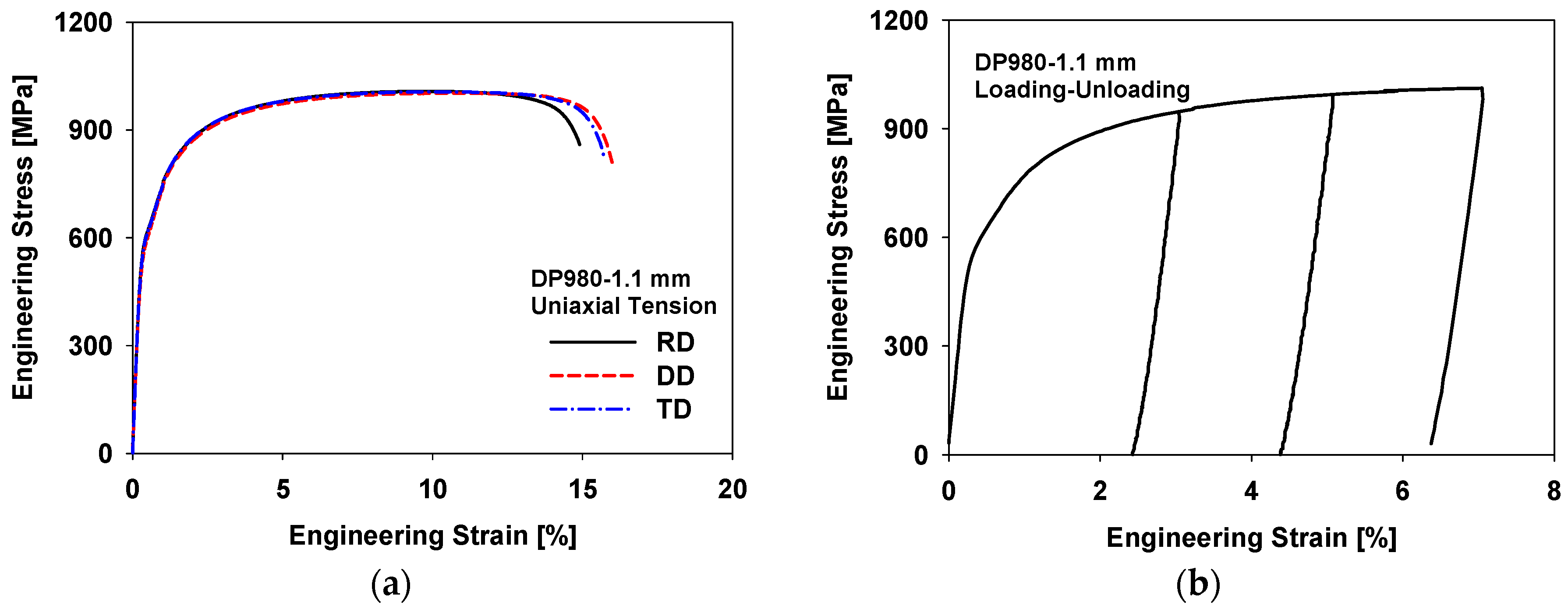
Figure 3.
Biaxial tensile test: (a) biaxial tensile tester; (b) cruciform specimen.
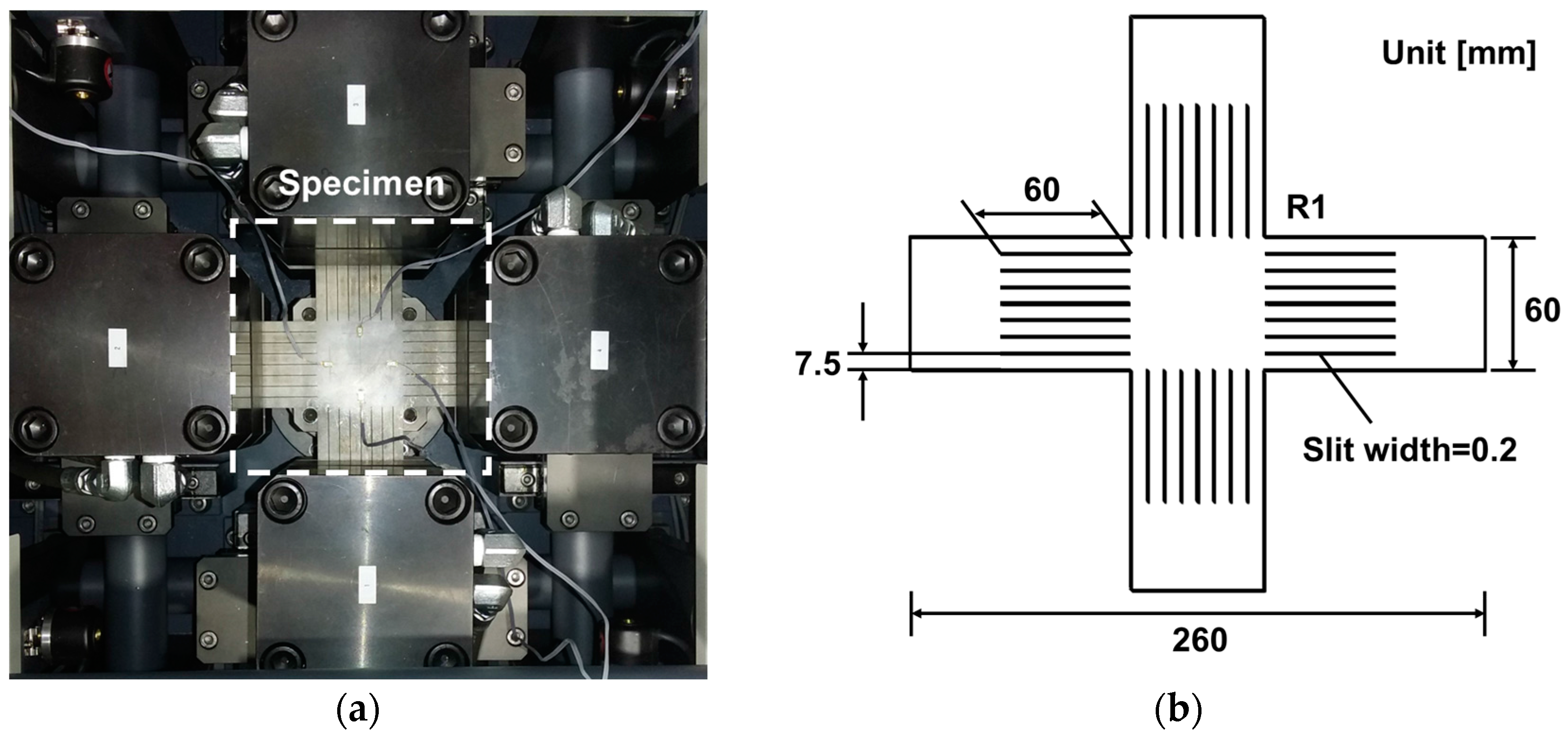
Figure 4.
Engineering stress–strain curves of the biaxial tension.

Figure 5.
(a) Variation of yield strength and (b) initial yield criteria.
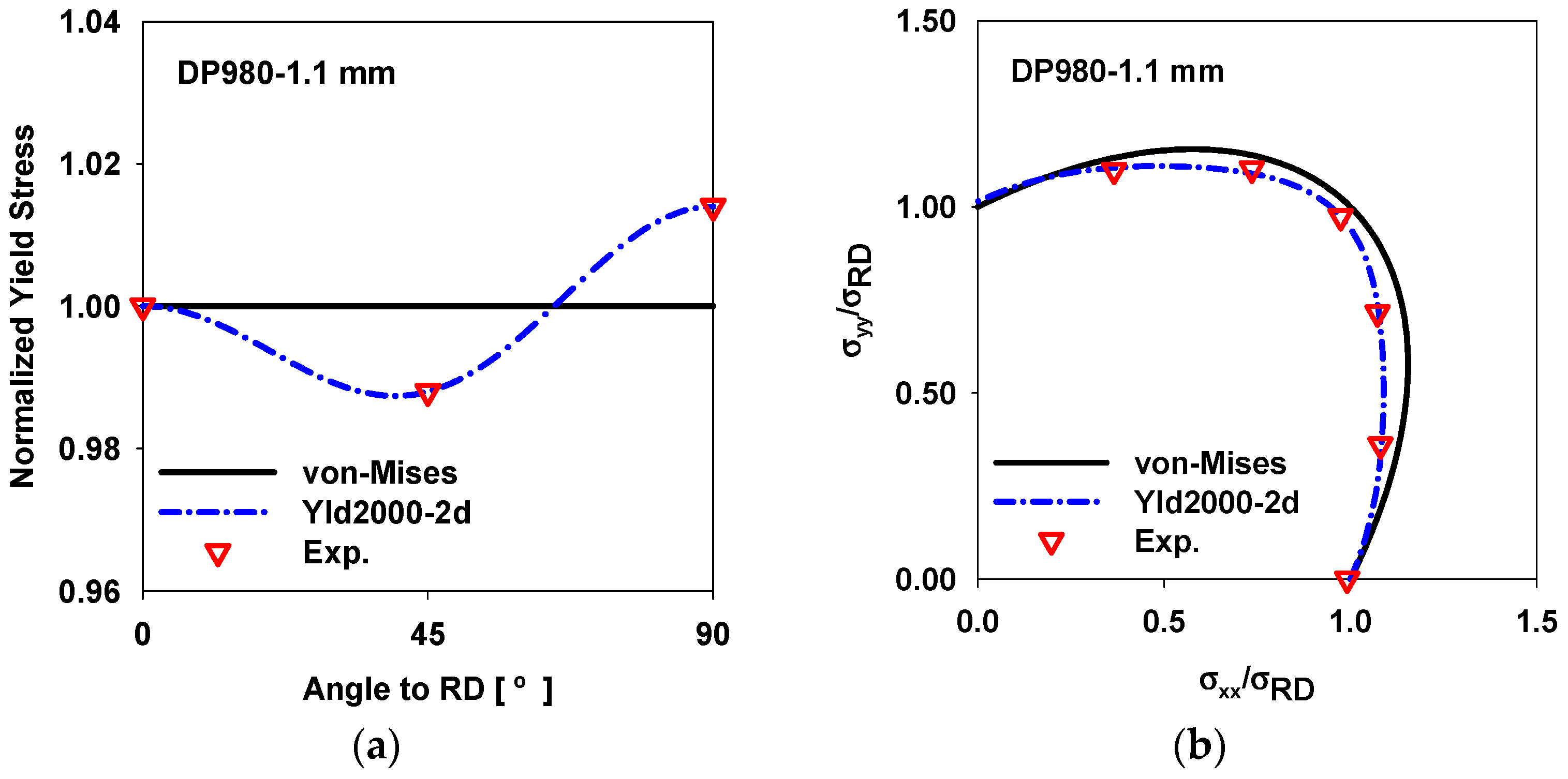
Figure 6.
The tension–compression test: (a) tension–compression tester; (b) specimen.
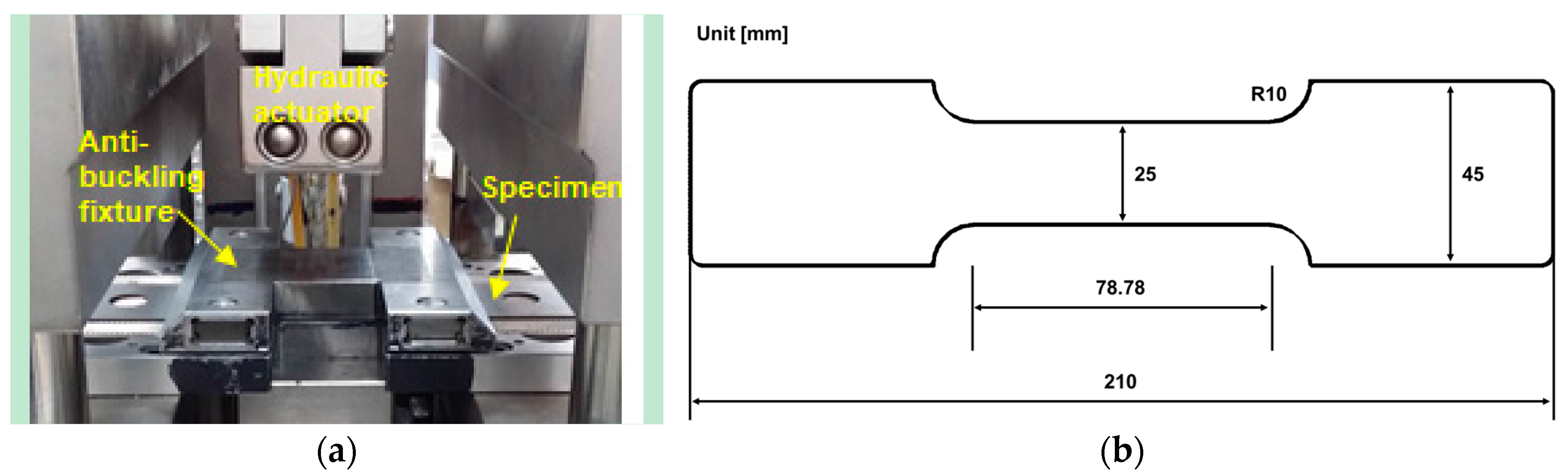
Figure 7.
Absolute true stress–accumulated plastic strain curves of the tension-compression tests.
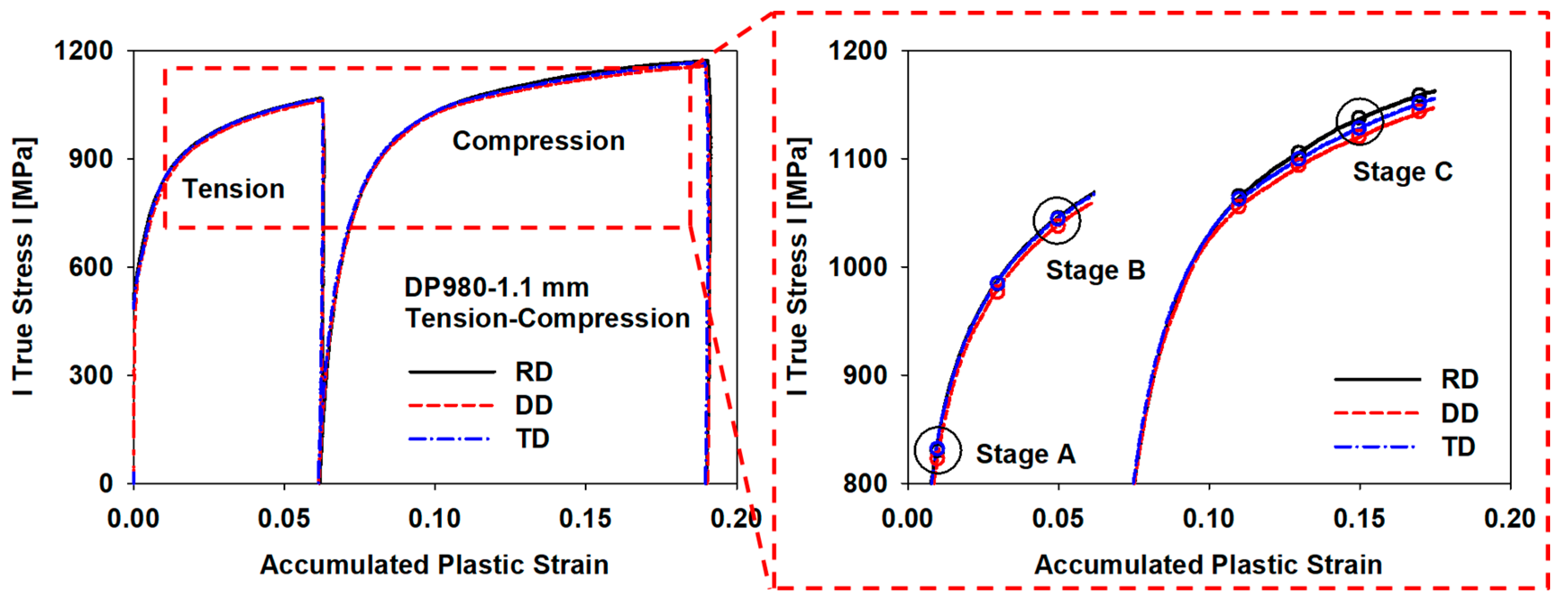
Figure 8.
Variation of anisotropy according to the hardening progress.

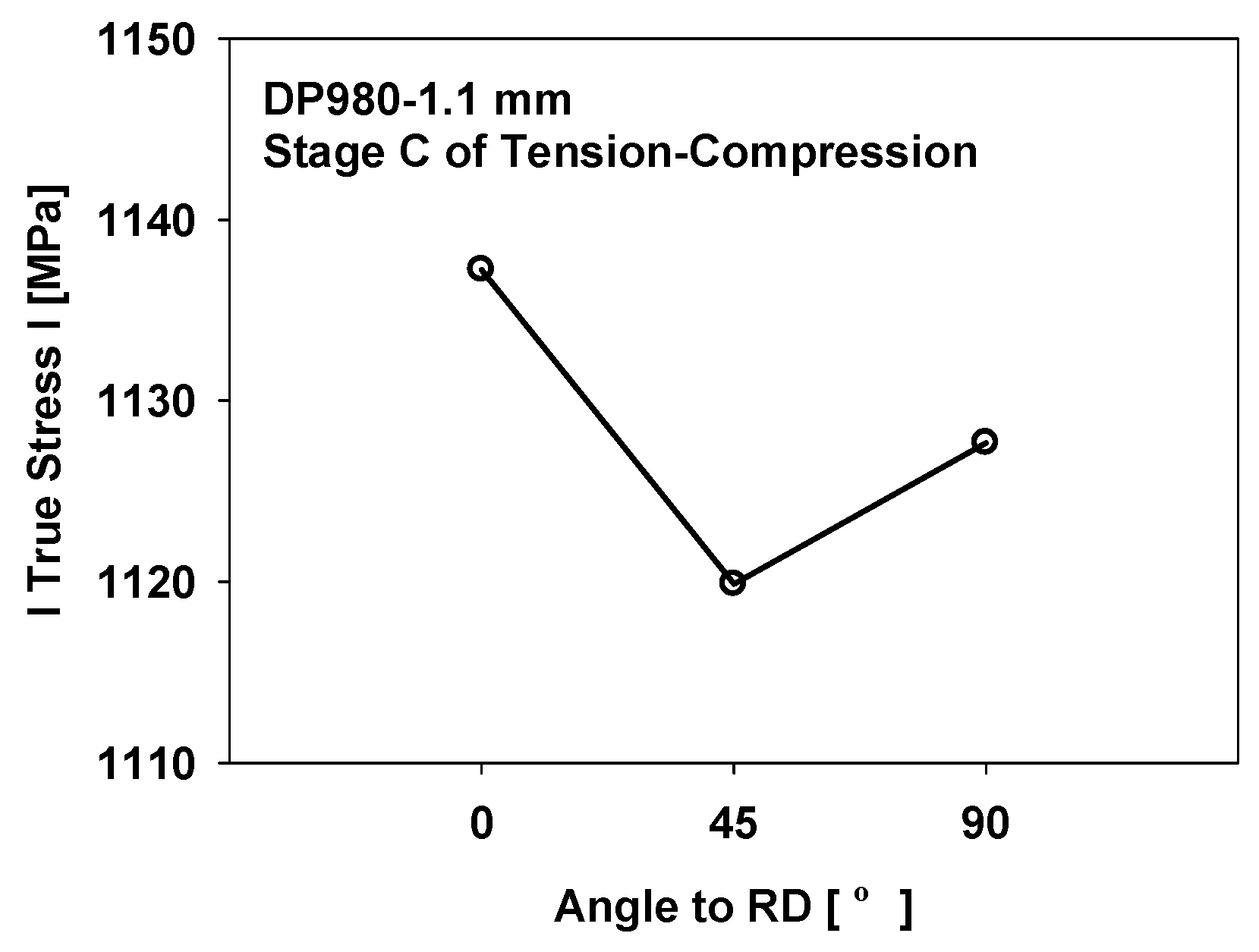
Figure 9.
True stress–strain curves under tension–compression calculated by the hardening models with (a) isotropic evolution and (b) anisotropic evolution.
Figure 9.
True stress–strain curves under tension–compression calculated by the hardening models with (a) isotropic evolution and (b) anisotropic evolution.
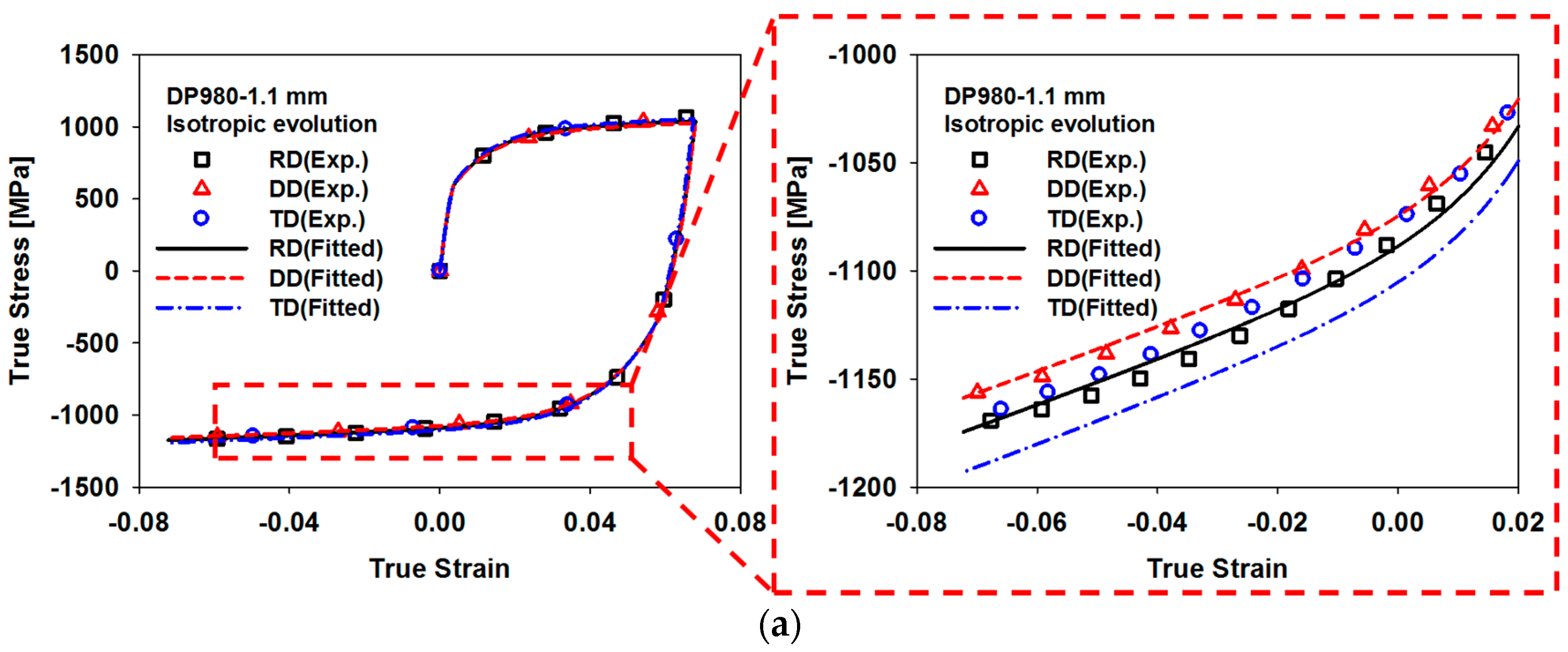

Figure 10.
Errors of fit of the isotropic and anisotropic evolution models.
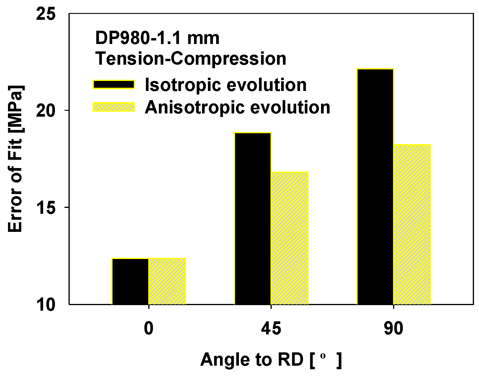
Figure 11.
U-bending test: (a) dimensions and (b) finite element model.
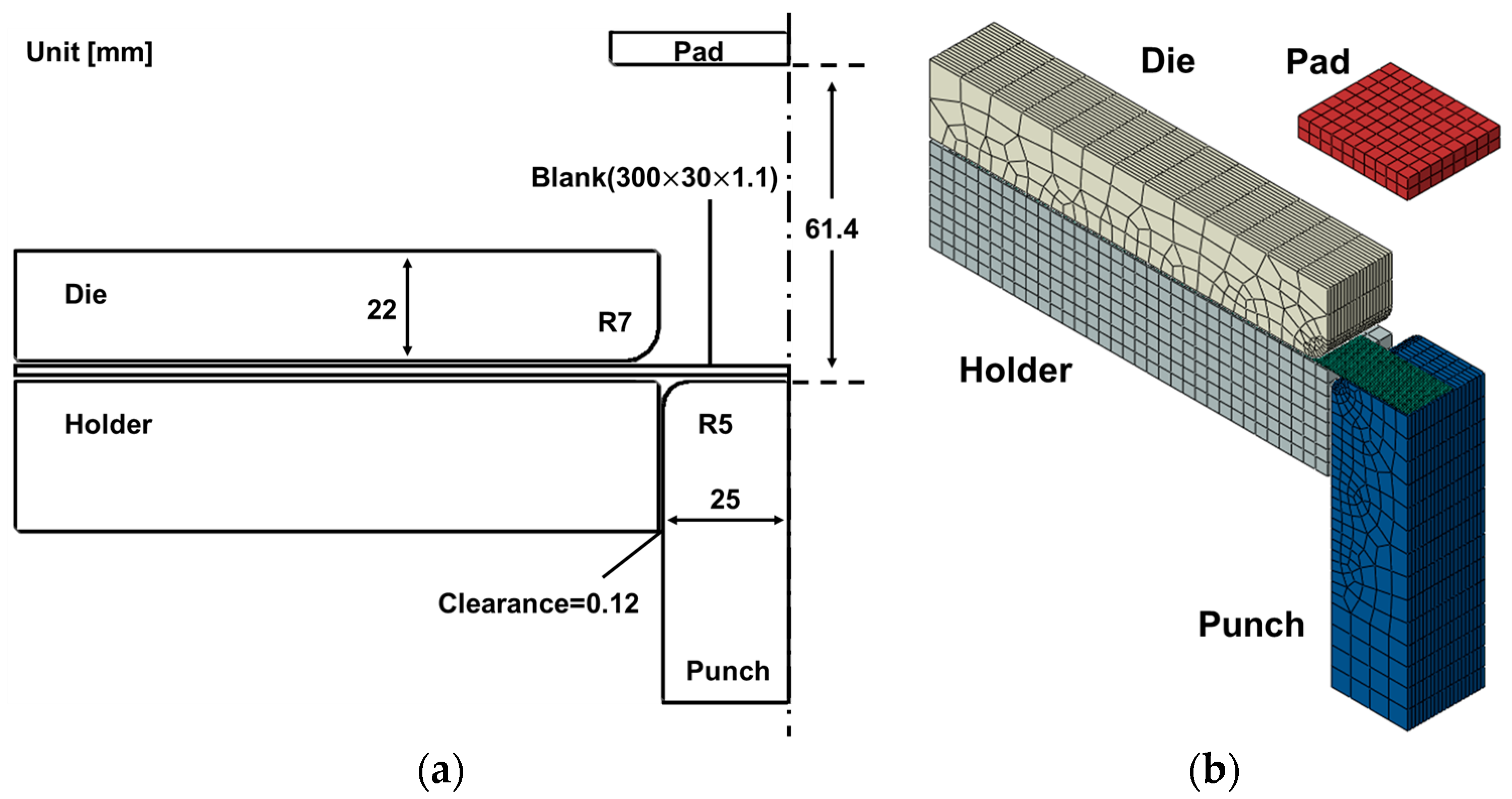
Figure 12.
(a) Specimens of the U-bending test and (b) measures of springback (, , and ).

Figure 13.
Intermediate shape after the springback for verification of difference between hardening models with isotropic and anisotropic evolution.
Figure 13.
Intermediate shape after the springback for verification of difference between hardening models with isotropic and anisotropic evolution.

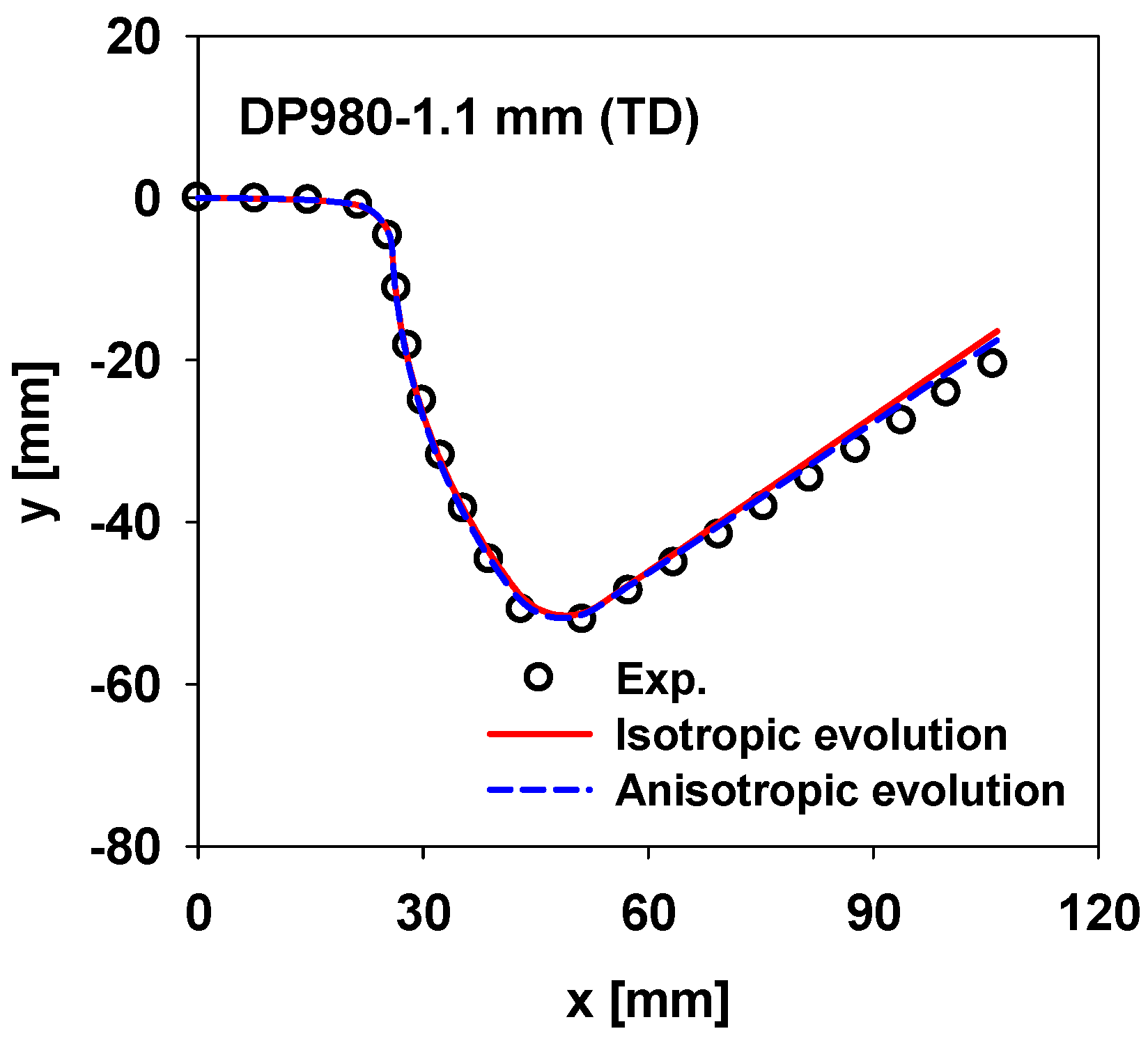
Figure 14.
Comparison of the measured and calculated springback measures: (a) curvature ; (b) springback angle ; (c) springback angle .
Figure 14.
Comparison of the measured and calculated springback measures: (a) curvature ; (b) springback angle ; (c) springback angle .

Table 1.
Uniaxial tensile properties of DP980.
| Direction | Young’s Modulus [GPa] | Yield Strength [MPa] | r-Value | Tensile Strength [MPa] | Elonagtion [%] |
|---|---|---|---|---|---|
| RD | 202.2 | 618.1 | 0.757 | 1014.1 | 15.6 |
| DD | 206.1 | 610.7 | 0.851 | 1015.6 | 16.4 |
| TD | 208.8 | 626.7 | 0.856 | 1021.9 | 14.0 |
Table 2.
Parameters of the QPE model.
| [GPa] | [GPa] | [MPa] | |
|---|---|---|---|
| 205.8 | 105.7 | 345 | 300 |
Table 3.
Balanced biaxial tensile properties of DP980.
| Elastic Modulus [GPa] | Yield Strength [MPa] | |
|---|---|---|
| 297.0 | 601.9 | 0.915 |
Table 4.
Parameters of the anisotropic Yld2000-2d yield function.
| 6 | 0.978 | 0.978 | 1.049 | 1.008 | 1.026 | 1.044 | 0.998 | 1.023 |
Table 5.
Parameters of hardening models with isotropic and anisotropic evolution.
| Hardening Model with Isotropic Evolution | ||||||||
| [MPa] | [MPa] | [MPa] | [MPa] | |||||
| 583.9 | 409.7 | 3.861 | 17,896 | 26,144 | 9.537 | 34.74 | 80.27 | 6.551 |
| Hardening Model with Anisotropic Evolution | ||||||||
| [MPa] | [MPa] | [MPa] | [MPa] | |||||
| 583.9 | 409.7 | 3.861 | 17,896 | 26,144 | 9.537 | 34.74 | 80.27 | 6.551 |
| 0.948 | 0.975 | 1.014 | 0.940 | |||||
© 2017 by the authors. Licensee MDPI, Basel, Switzerland. This article is an open access article distributed under the terms and conditions of the Creative Commons Attribution (CC BY) license (http://creativecommons.org/licenses/by/4.0/).
Share and Cite
MDPI and ACS Style
Jung, J.; Jun, S.; Lee, H.-S.; Kim, B.-M.; Lee, M.-G.; Kim, J.H. Anisotropic Hardening Behaviour and Springback of Advanced High-Strength Steels. Metals 2017, 7, 480. https://doi.org/10.3390/met7110480
AMA Style
Jung J, Jun S, Lee H-S, Kim B-M, Lee M-G, Kim JH. Anisotropic Hardening Behaviour and Springback of Advanced High-Strength Steels. Metals. 2017; 7(11):480. https://doi.org/10.3390/met7110480
Chicago/Turabian StyleJung, Jaebong, Sungwook Jun, Hyun-Seok Lee, Byung-Min Kim, Myoung-Gyu Lee, and Ji Hoon Kim. 2017. "Anisotropic Hardening Behaviour and Springback of Advanced High-Strength Steels" Metals 7, no. 11: 480. https://doi.org/10.3390/met7110480
Note that from the first issue of 2016, this journal uses article numbers instead of page numbers. See further details here.