Tensile–Shear Fracture Behavior Prediction of High-Strength Steel Laser Overlap Welds

Abstract

A wider interface bead width is required for laser overlap welding by increasing the strength of the base material (BM) because the strength difference between the weld metal (WM) and the BM decreases. An insufficient interface bead width leads to interface fracturing rather than to the fracture of the BM and heat-affected zone (HAZ) during a tensile–shear test. An analytic model was developed to predict the tensile–shear fracture location without destructive testing. The model estimated the hardness of the WM and HAZ by using information such as the chemical composition and tensile strength of the BM provided by the steel makers. The strength of the weldments was calculated from the estimated hardness. The developed model considered overlap weldments with similar and dissimilar material combinations of various steel grades from 590 to 1500 MPa. The critical interface bead width for avoiding interface fracturing was suggested with an accuracy higher than 90%. Under all the experimental conditions, a bead width that was only 5% larger than the calculated value could prevent the fracture of the interface.

1. Introduction

In the automotive industry, the use of high-strength steel is increasing, and the importance of a lightweight car body is becoming more prominent because of CO₂ emission regulations. The most recently developed high-strength steels utilize a martensite phase as the hardest steel phase [1,2,3], and even fully martensitic steel, such as hot-press forming steel and martensitic steel, are being adopted as materials of the central pillar, bumper beam, and several reinforcement parts [4,5].

Welding is the main joining process of an automotive steel structure [6], and resistance spot welding, gas metal arc welding, and laser welding are the most frequently used welding processes for automotive steel sheets. When welding a conventional mild steel, the weld metal (WM) and heat-affected zone (HAZ) are subjected to a high cooling rate during the solidification and their microstructures become harder than those of the base material (BM). For the case of high-strength steel containing martensite, the strength difference between the WM and BM was reduced, even though the WM can almost become fully hardened by laser welding [7]. Because the martensite fraction within the BM increases, the strength of BM becomes higher. HAZ softening can be observed, owing to the tempering of martensite even by laser welding, which is a low-heat-input process [8,9,10,11].

The hardness profile of the weldment can be adopted to predict the strength of the weldment and crack susceptibility. Several carbon equivalents have been proposed to estimate the hardness of the WM and HAZ. The international institute of welding adopted a carbon equivalent based on the Dearbon and O’Neil formula [12] for plain carbon and carbon-manganese steels in 1967. Ito and Bessyo [13] suggested a critical metal parameter, Pcm, to estimate HAZ cracking susceptibility for low alloy steel. A carbon equivalent suitable for a wide range of carbon contents was developed by Yurioka et al. [14,15]. Kasuya et al. [16,17] evaluated various carbon equivalents to predict the maximum hardness of HAZ. Carbon equivalents regarding laser welding have also been proposed in previous studies. Kaizu et al. [18] and Taka et al. [19] simplified the Pcm formula using experimental approaches and suggested carbon equivalent models dedicated to laser welding. Uijl et al. [20] evaluated carbon equivalents for various welding processes including laser welding. The authors modified Kaizu’s carbon equivalent equation [18] to extend the hardness prediction model such that it would include boron steels [21].

The weldment hardness profile represents the local strength along the weldment. In a previous study [11], the authors conducted a tensile test for laser butt-welded specimens with various grade strengths from 340 to 1500 MPa. The fracture locations were in good agreement with the minimum hardness location, except in the case of the 780 MPa grade, in which the HAZ was narrow enough and the HAZ softening was relatively small, owing to laser welding. Additionally, for a tensile–shear test, the hardness profile can be used to estimate the shear strength of the WM and the tensile strength of the HAZ and BM. Because the shear strength of a material is 1.73–2 times lower than its tensile strength, a higher hardness and/or wider interface bead width are required to avoid the interface fracture (IF) in a tensile–shear test. In the laser welding of mild steel, the hardness of the WM is more than twice as high as that of the BM [11,22] and BM fracturing is easily observed in the tensile–shear test [23]. However, for ultrahigh-strength steel, such as hot-press-forming steel with a strength of 1.5 GPa, the welding parameters of BM or HAZ fracturing can hardly be obtained because the WM will no longer be harder than the BM; laser welding will naturally be employed to reduce the heat input and consequently the IF bead width [24].

The rotation of the specimen during the tensile–shear test makes it more difficult to predict the fracture location [25,26]. Ono et al. [27] established an analytic model to predict the fracture location based on the given tensile strength of the BM, measured hardness of the WM, and IF bead width. Furisako et al. [26] classified the fracture location into a BM, WM, and curvature portion between the BM and WM, and suggested an analytic fracture model based on the hardness measurement and a regression model for the rotation angle [23,26]. Benasciutti et al. [25] established a simple model by considering the rotation angle and weldment properties. Their model was thereby expanded to include circular beads. Various numerical models have also been reported, with a consideration of complex loading conditions and with the objective of predicting the behavior of the specimen and the fracture mode during the tensile–shear test of a laser lap-welded specimen. Terasiki et al. [28] proposed the numerical model to predict the static fracture strength of a laser lap-welded specimen. Also, by using finite element analyses, the ductile fracture initiation and necking phenomena were simulated during the tensile-shear test of high strength low alloy steel sheets [29,30]. Ha et al. [31] developed a failure criterion under combined normal and shear loading conditions for laser welds by experimental approaches and numerical analyses. Ma et al. [32] numerically simulated the tensile-shear test of the high strength dual phase 980 steel weldments considering the hardened and the softened zones within the specimen.

For industrial use, a simple and analytic model rather than a numerical model is preferred, as long as the prediction accuracy is guaranteed to some extent [33]. In this study, an integrated model is proposed to predict the hardness of the weldment and the fracture location in the tensile–shear test of a laser lap weldment. Extensive material combinations of overlap welding were considered by using high-strength steel grades between 590 MPa and 1.5 GPa. The hardness of each weld was measured and was additionally estimated by a carbon equivalent that was calculated by the chemical compositions of the mill sheets supplied by the mill makers. The fracture locations that were observed in the tensile–shear test were predicted by an analytic model and compared with the experimental results.

2. Experimental Procedure

Laser overlap welding was applied to various grades of high-strength steel. The specimen was machined with a width of 120 mm and length of 150 mm. All the sheets had a thickness of 1.2 mm, except for the HPF 1500 steel, which had a thickness of 1.1 mm. For all dissimilar joints, the lower-strength steel sheets were placed on top. Uncoated sheets were chosen to eliminate the influence of the coating layer’s chemical composition. The chemical compositions of the applied materials, such as that of the mill sheet provided by the steel makers, are presented in

Table 1. Chemical composition of base materials listed on the mill sheet from the steel maker (wt. %).

Base Materials	C	Si	Mn	P	S	Cr	B
590 DP (1.2 mm)	0.078	0.363	1.808	0.011	0.001	-	-
780 DP (1.2 mm)	0.070	0.977	2.264	0.010	0.015	-	-
980 DP (1.2 mm)	0.170	1.340	2.000	0.016	0.001	-	-
1180 CP (1.2 mm)	0.110	0.110	2.790	0.019	0.004	1.040	-
1500 HPF (1.1 mm)	0.216	0.240	1.255	0.002	0.002	0.001	0.003

. The carbon content increased by increasing the strength, except for the 1180 CP steel. In this study, a total of 15 combinations of the five BMs was considered to obtain the various carbon equivalent conditions (

Table 2. Material combination for case study; (a) similar and (b) dissimilar.

(a)
Specimen.	Top Plate	Top Plate
S6/6	CR 590 DP	CR 590 DP
S8/8	CR 780 DP	CR 780 DP
S10/10	CR 980 DP	CR 980 DP
S12/12	CR 1180 CP	CR 1180 CP
S15/15	HPF 1500	HPF 1500
(b)
Specimen.	Top Plate	Bottom Plate
D6/8	CR 590 DP	CR 780 DP
D6/10	-	CR 980 DP
D6/12	-	CR 1180 CP
D6/15	-	HPF 1500
D8/10	CR 780 DP	CR 980 DP
D8/12	-	CR 1180 CP
D8/15	-	HPF 1500
D10/12	CR 980 DP	CR 1180 CP
D10/15	-	HPF 1500
D12/15	CR 1180 CP	HPF 1500

). The welding speed (16–72 mm/s) and focal position (0–20 mm) were variably combined to obtain a diverse bead width at the interface. Laser weldments were fabricated for six cases per material combination with various combinations of welding speeds and focal positions (

Table 3. Specification of the applied laser beam depending on the focal position, and heat input at a differential welding speed.

Parameters	Level 1	Level 2	Level 3	Level 4	Level 5	Level 6
Focal position (mm)	0	5	10	10	15	20
Laser spot size (mm)	0.3	0.34	0.46	0.46	0.55	0.65
Apparent power density (W/mm2)	13,440	10,463	5716	5716	3999	2863
Welding speed (mm/s)	70	60	48	37	26	20
Heat input per unit length (J/mm)	54.3	63.3	79.2	102.7	146.2	190.0

).

A continuous mode Yb:YAG disk laser HLD 4002 (Trumpf, Ditzingen, Germany) was applied to the welding. The laser beam was delivered through an optical fiber with a diameter of 200 µm and optic system PFO33 (Trumpf, Ditzingen, Germany). The delivered beam was collimated (length of collimation: 150 mm) and focused (focal length: 450 mm), which resulted in a focal diameter of 0.6 mm with a beam quality (beam parameter product) of 8.5 mm·rad. The beam was irradiated perpendicularly onto the workpiece under 3.5 kW of laser power. Shielding gas was not provided during the welding [34].

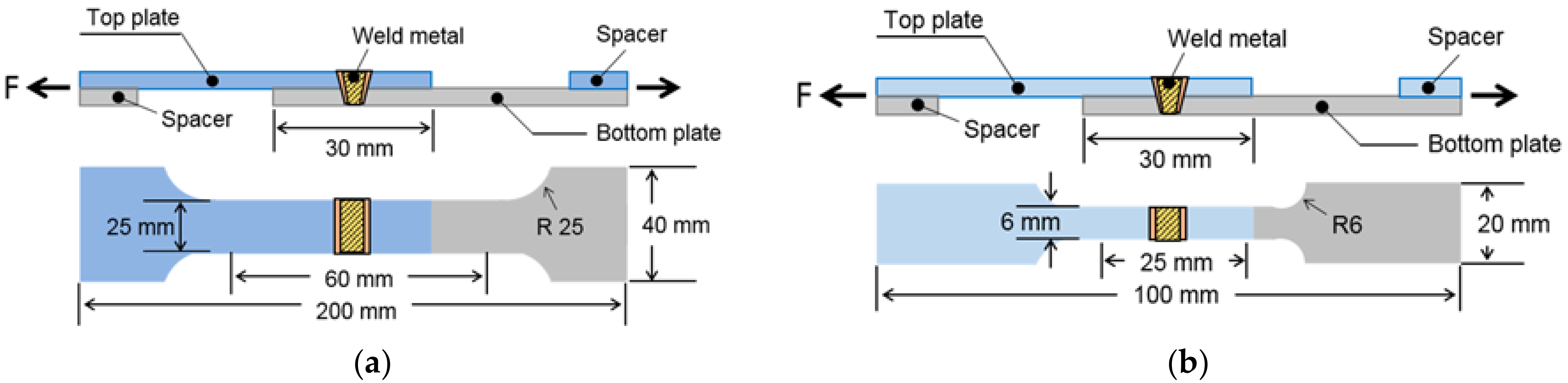
After the laser overlap welding, each specimen was polished and etched with 1% of nital solution to measure the width of the interfacial surface. The tensile–shear test specimens were obtained from the overlap-welded specimen. Additionally, the dimensions of each workpiece were prepared with a gage length of 60 mm and a parallel width of 25 mm, as shown in Figure 1a. Each tensile–shear test specimen was tested three times and the average value was calculated.

To measure the rotation angle during the tensile–shear test, a digital image correlation (DIC) technique and high-speed camera UX50 (Photron, San Diego, CA, USA) were used. The specimen was machined based on the ASTM E8 standard for a subsize specimen with a gage length of 25 mm and a parallel width of 6 mm (Figure 1b). During the tensile–shear test, DIC was applied to the analysis of the three-dimensional deformation of the upper surface. The high-speed camera was installed to obtain a side-view video with a frame rate of 50 frames per second. The Vickers hardness values were measured in all cases, and a line profile was obtained with a step size of 200 µm and load of 0.98 N, according to the ASTM E384-99 standard.

3. Results and Discussion

3.1. Laser Weld Characteristics under Various Welding Conditions

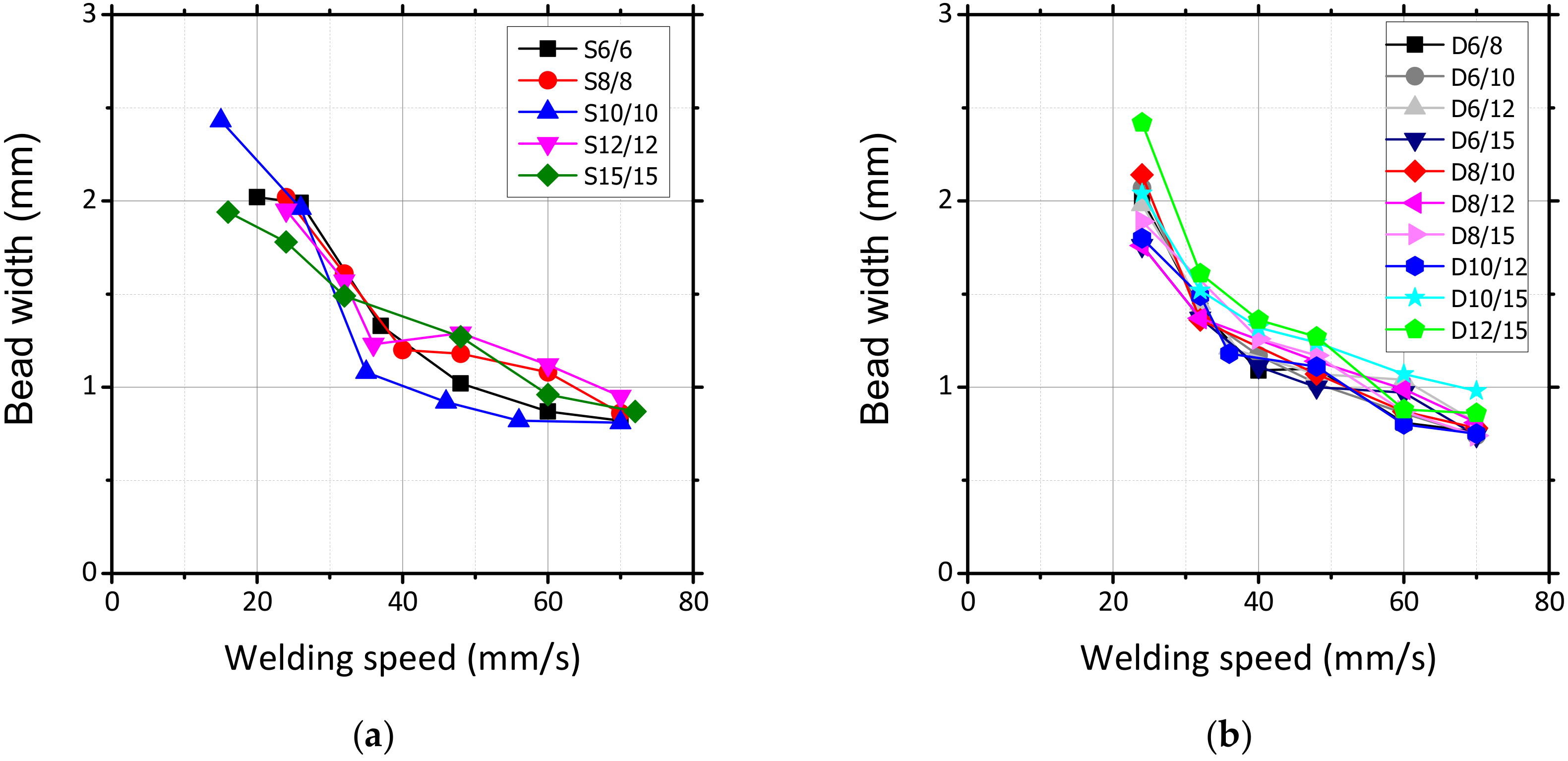
The bead width is subject to welding parameters such as the laser power, welding speed, and focal position. In the experiments, the laser power was fixed at 3.5 kW. The focal position was set from 0 to 20 mm at intervals of 5 mm, and the welding speed was set between 20 and 70 mm/s to achieve a fully penetrated bead for the given focal position. A larger IF width was produced at slower welding speeds, in comparison to that produced at faster welding speeds (Figure 2). Although a wide WM and HAZ were generated under lower-welding-speed conditions because of the relatively high heat input, the average hardness within the WM and minimum hardness within the HAZ, which determines the HAZ failure, were almost constant regardless of the heat input (Figure 3). These results are in good agreement with the study of Han et al. [7].

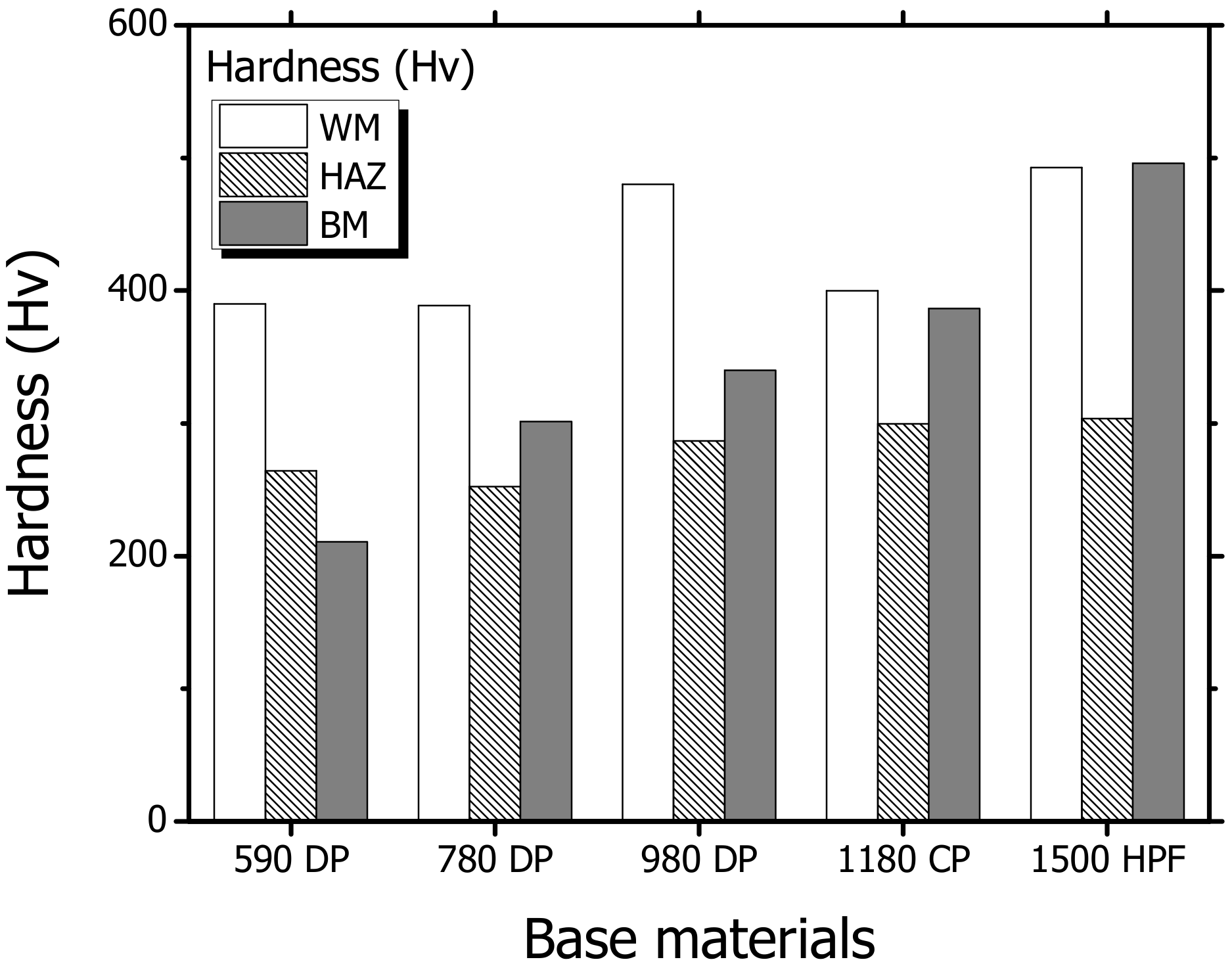
The hardness profiles were determined by the thermal history and chemical composition of the BM. The HAZ had a much lower hardness than the WM in all cases, and even lower hardness than the BM, except for the 590 DP steel (Figure 4). The HAZ softened from 61 to 84% in comparison to the BM, and originated from the tempering of martensite in high-strength steel [11]. For the 1500 HPF steel with a strength of 1.5 GPa, which was designated to a hot-press forming process, the hardness values of the WM and BM were similar. However, the hardness of the HAZ degraded to 61% of the BM hardness.

3.2. Fracture Mode Definitions for Overlap Welds

Figure 5 shows the classification of the overlap joint’s failure mode, which can be classified as a BM fracture, IF fracture, or HAZ fracture, depending on the ruptured location. Because the load was consistent along the longitudinal direction of a specimen, a comparison between the shear load on the IF ($F_{\mathrm{WM}}$) and tensile load on the BM or HAZ ($F_{\mathrm{BM}} \mathrm{or} F_{\mathrm{HAZ}}$) was conducted to determine whether an IF fracture occurs, where ${\mathsf{\tau }}_{\mathrm{WM}}$ is the shear stress at the interface; θ is the angle of the weld rotation; L_IF is the interface bead width; t and w are the thickness and width of the specimen, respectively; and ${\mathsf{\sigma }}_{\mathrm{BM}}$ and ${\mathsf{\sigma }}_{\mathrm{HAZ}}$ are the tensile stresses of the BM and HAZ, respectively. Accordingly, the failure mode could be predicted from the determined values of θ, $L_{\mathrm{IF}}$, ${\mathsf{\tau }}_{\mathrm{WM}}$, and ${\mathsf{\sigma }}_{\mathrm{HAZ}}$, where w and t were fixed.

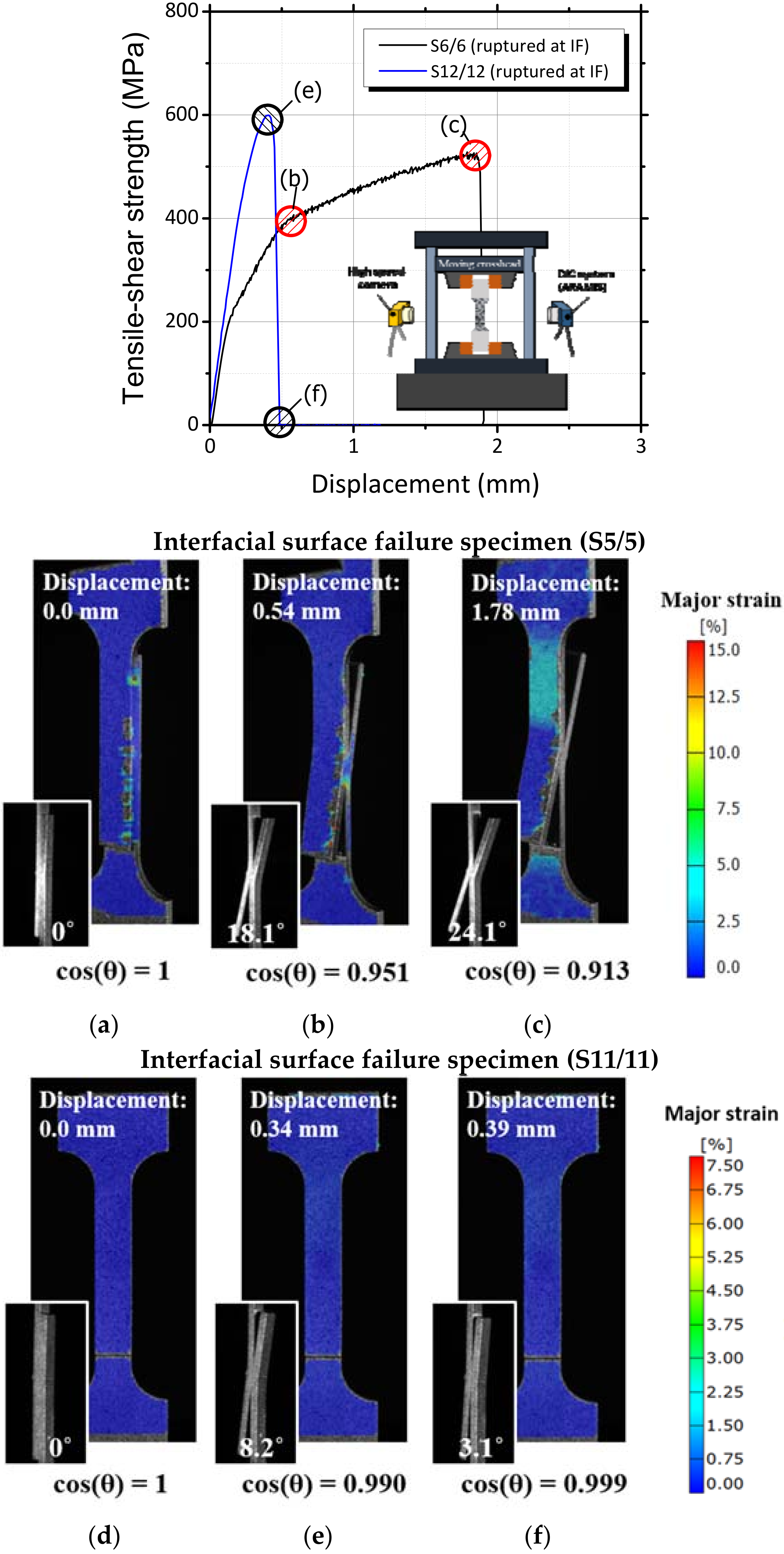
The rotation angle θ during the tensile–shear test is related to the ductility of the weldment and was observed using a DIC system and high-speed camera for the tensile–shear test of the 590 DP and 1180 CP specimens. The test results of the IF fracture are presented in Figure 6. In the experiments, the 590 DP steel showed the highest ductility. In the test of the 590 DP specimen, the specimen reached the yield point when the rotation angle was 18.1° (Figure 6) and deformed plastically with a rotation angle of 24.1° until it finally ruptured (Figure 6c). Regardless of the relatively high elongation, the measured value of cos(θ) exceeded 0.951 at the yield point. In the DIC images of the 1180 CP steel that ruptured at the interface, the rotation angle at the maximum tensile–shear load was confirmed as 8.2°, and cos(θ) was almost 1 (Figure 6e). This means that the high-strength steel specimen barely rotated during the tensile–shear test. After the fracture, the rotation angle recovered to 3.1° and insignificant deformation was also observed in the DIC images (Figure 6f). In the DIC and high-speed camera images, the tensile-mode strain was observed to be negligible and the specimen mainly exhibited shear mode fracturing.

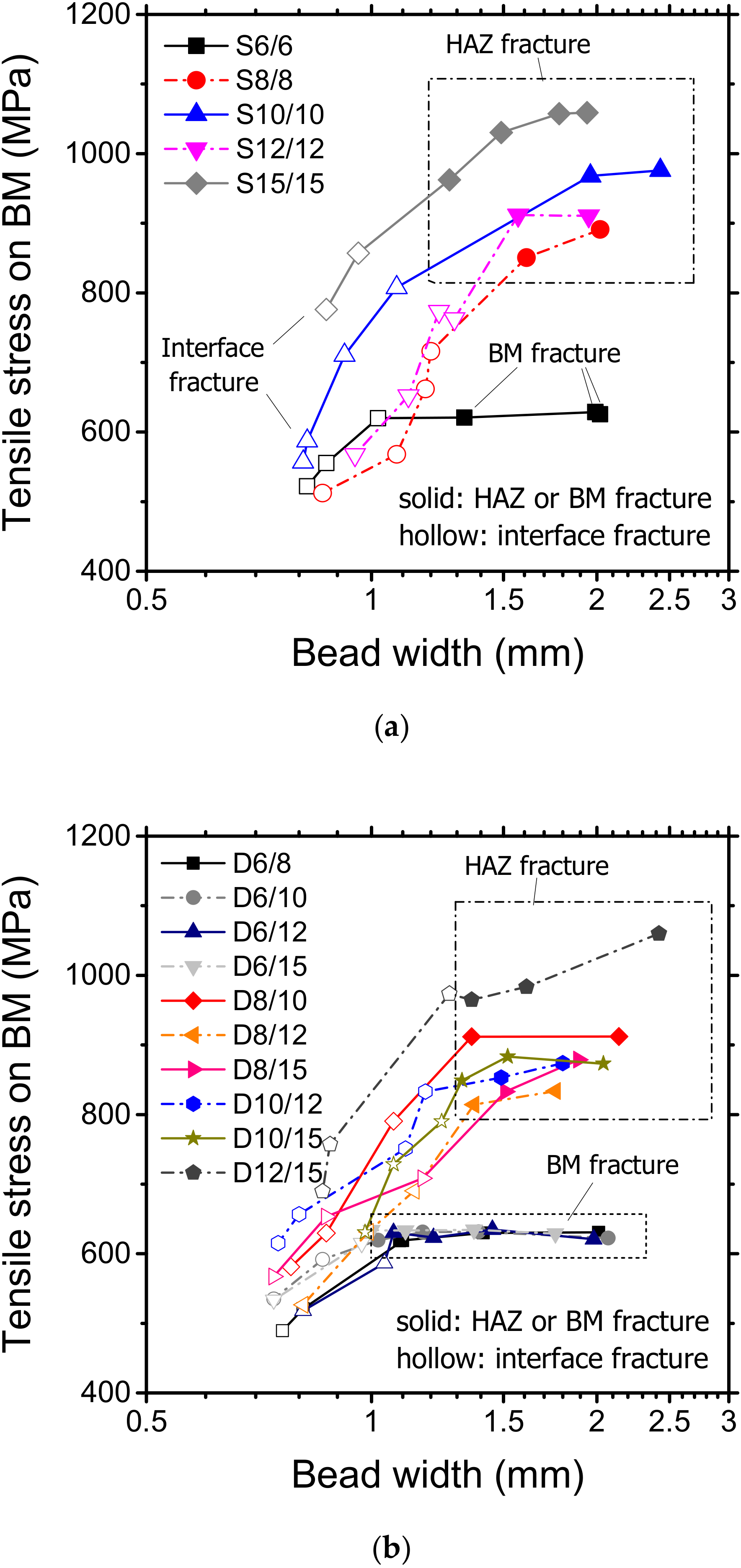
The fracture mode changed from IF to BM (or HAZ) by increasing the IF bead width (Figure 7). The IF bead width and tensile stress for the transition varied according to the strength of the materials. For the 590 DP steel, the fracture location moved from the IF to the BM by increasing the IF bead width. While in other cases, it moved from the IF to the HAZ, which had the lowest hardness, as can be observed in Figure 4. For dissimilar material combinations, a wider IF bead could prevent the IF fracture. For a sufficient IF width, whether the fracture location was the BM or HAZ was predominantly affected by a lower-strength counterpart steel (Figure 7b). In the case of the combination with 590 DP steel, the fracture location moved from the IF to the BM by increasing the IF bead width while the others were fractured at the HAZ.

3.3. Estimation of Hardness with Carbon Equivalent

The hardness of the weldment was determined by the chemical composition and thermal history. Laser welding enables a low heat input during welding and the hardness of the WM can be increased similarly to that of a water-quenched specimen [7]. As shown in Figure 3, the average hardness within the WM and the minimum hardness of the HAZ were maintained, even for different welding speeds and resultant heat inputs. Therefore, in this study, the hardness of the WM was only estimated by the chemical compositions of the BM rather than by the thermal history. The carbon equivalent proposed in the authors’ previous study [21] was adopted in order to estimate the strength of the welds Equation (1). This was established based on Kaizu’s equation, which was derived from laser welding, and modified to consider the boron in the hot-press forming steel. The prediction of the Vickers hardness ($H{v}_{\mathrm{WM}}$) was carried out with a consideration of the carbon equivalent, as expressed by Equation (2), [7]. For a dissimilar material combination, the carbon equivalent assumed that the two steel sheets were diluted with a ratio of 1:1.

$$C{E}_{\mathrm{LB}}=\mathrm{C} + \mathrm{Si}/50 + \mathrm{Mn}/25 + \mathrm{P}/2 + \mathrm{Cr}/25 +14\mathrm{B}$$

(1)

where C, Si, Mn, P, Cr, and B represent the weight percentage of carbon, silicon, manganese, phosphorus, chrome, and boron, respectively.

$$H{v}_{\mathrm{WM}}=701 C{E}_{LB} +281$$

(2)

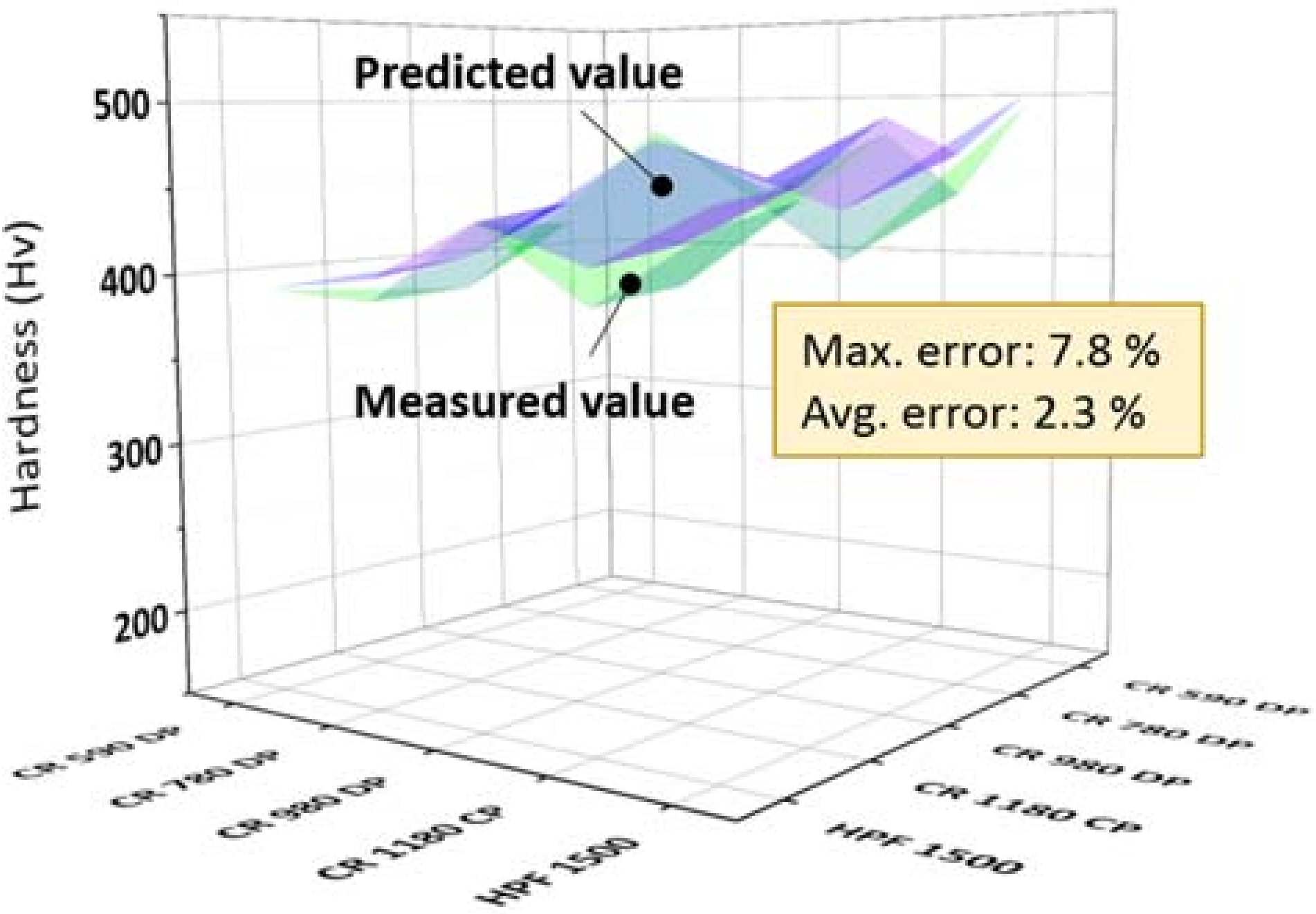
The predicted hardness values obtained from the carbon equivalent were compared with the experimental values (Figure 8 and

Table 4. Estimated hardness values of weld metals for (a) similar and (b) dissimilar material joints using carbon equivalents.

(a)
Specimen	S6/6		S8/8		S10/10		S12/12		S15/15
Measured hardness (Hv)	390.0		388.8		480.0		399.9		492.7
Predicted hardness (Hv)	391.4		407.1		475.0		431.0		499.7
CELB	0.157		0.180		0.277		0.214		0.312
Error (%)	0.4		4.7		1.0		7.8		1.4
(b)
Specimen	D6/8	D6/10	D6/12	D6/15	D8/10	D8/12	D8/15	D10/12	D10/15	D12/15
Measured hardness (Hv)	386.6	432.2	390.4	434.0	429.4	396.4	445.6	446.0	478.4	442.2
Predicted hardness (Hv)	399.3	433.2	411.2	445.5	441.1	419.0	453.4	453.0	487.4	465.3
Error (%)	3.3	0.2	5.3	2.6	2.7	5.7	1.8	1.6	1.9	5.2

). The average prediction error was 2.3% and the maximum prediction error was 7.8%. The discrepancy was relatively high for similar and dissimilar material combinations with 1180 CP steel.

After the laser welding, a differential amount of HAZ softening was observed according to the strength of the BM (Figure 4). The HAZ softening could be predicted in a more sophisticated way, in comparison to the WM hardness prediction. The HAZ consisted of three phases; namely, martensite, bainite, and ferrite/pearlite. The hardness of the HAZ (Hv_HAZ) could be estimated by using the rule of mixtures [35] for three phases, by using the volume fraction of each phase and its hardness, as expressed by the following equation:

$$H{v}_{\mathrm{HAZ}}=H_{\mathrm{m}}{V}_{\mathrm{m}}+H_{\mathrm{b}}{V}_{\mathrm{b}}+H_{\mathrm{fp}}{V}_{\mathrm{fp}}$$

(3)

where H_m, H_b, and H_fp represent the hardness values of martensite, bainite, and ferrite/pearlite in the HAZ, respectively; and V_m, V_b, and V_fp represent their volume fractions in the HAZ, respectively.

The hardness and volume fraction of each phase were determined by the thermal history and chemical composition of the BM. In this study, Ion’s mathematical model [35] was employed in the calculations. The phase fraction and its hardness were calculated for each BM and are presented in

Table 5. Estimated hardness values of the heat-affected zone for used materials: (a) calculated phase fractions and hardness values based on Ion’s equations; (b) comparison of experimentally obtained hardness values with mathematically obtained results.

(a)
Phase fraction	Hm	Hb		Hf		Vm		Vb		Vfp
590 DP	357.95	290.27		151.67		0.44		0.06		0.50
780 DP	371.86	292.97		125.34		0.47		0.03		0.50
980 DP	473.84	337.26		117.19		0.55		0.02		0.43
1180 CP	383.16	321.56		201.17		0.53		0.01		0.46
1500 HPF	479.80	349.89		173.57		0.54		0.04		0.42
(b)
Base metal	590 DP		780 DP		980 DP		1180 CP		1500 HPF
Measured hardness (Hv)	264.2		252.2		286.8		299.7		303.6
Predicted hardness (Hv)	250.2		247.2		317.7		298.2		345.8
Error (%)	5.3		2.0		10.8		0.5		13.9

a. The carbon equivalent increased as the strength of the BM increased. Then, the fraction of the martensite phase that was calculated from the carbon equivalent also increased. The average error was 6.5%, and the standard deviation was 5.7%. The maximum error between the measured and predicted value was 13.9% in the case of the 1500 HPF. The hardness prediction for the HAZ was less accurate in comparison with the WM, owing to the limitations of the mathematical model, because the theoretical model did not consider the initial state of the materials, such as the primary grain size, and manufacturing processes such as the rolling and heat treatment. The prediction models of the HAZ are steadily evolving and will be improved in future work.

3.4. Critical Interface Bead Width (L_IF)

The critical IF bead width (L_C) to avoid the IF fracture was provided by the analytic model. The relationships between the load, stress, and geometry are shown in Figure 5. Additionally, L_C could be calculated by the force balance, as follows:

$$L_{\mathrm{c}}=\left[\min \left(T{S}_{\mathrm{HAZ}},T{S}_{\mathrm{BM}}\right)\times t\right]/\left[{\mathsf{\tau }}_{\max ,\mathrm{WM}}\times \cos \mathsf{\theta }\right]$$

(4)

where ${\mathsf{\tau }}_{\max ,\mathrm{WM}}$ is the shear strength of the WM; and TS_HAZ and TS_BM represent the tensile strengths of the HAZ and BM, respectively.

When the yield occurred at the WM during the tensile–shear test, the cosine value of the rotation angle was over 0.95, as shown in Figure 6. In the calculation, cos(θ) was approximated as 1. The measured tensile strength of the BM (TS_BM) was provided to the mill sheets. The tensile strength, TS, could be estimated from the Vickers hardness, Hv, by $TS=54+2.2969\times Hv$ [36]. TS_HAZ was calculated based on the HAZ hardness prediction, as was previously suggested in Section 3.3. The shear strength of the WM (${\mathsf{\tau }}_{\max ,\mathrm{WM}}$) was derived as follows:

$${\mathsf{\tau }}_{\max ,\mathrm{WM}}=T{S}_{\mathrm{WM}}/\surd 3=\left(54+2.2969\times H{v}_{\mathrm{WM}}\right)/\surd 3$$

(5)

where TS_WM and Hv_WM are the tensile strength and Vickers hardness of the WM, respectively.

The strength of each weld was obtained by applying the formula presented in

Table 6. Estimated tensile strength of base materials and heat-affected zone and shear strength of the weld metal: (a) similar material combination; (b) dissimilar material combination.

(a) Similar Material Combination
Specimen	S6/6		S8/8		S10/10		S12/12		S15/15
$T{S}_{\mathrm{BM}-\mathrm{as}\mathrm{recieved}}$	609.0		816.5		1023.3		1272.7		1545.0
$T{S}_{\mathrm{HAZ}-\mathrm{calc}.}$	817.4		807.4		1037.8		974.0		1129.5
${\mathsf{\tau }}_{\max ,\mathrm{WM}-\mathrm{calc}.}$	738.2		767.8		895.9		812.9		942.4
(b) Dissimilar Material Combinations
Specimen	D6/8	D6/10	D6/12	D6/15	D8/10	D8/12	D8/15	D10/12	D10/15	D12/15
$T{S}_{\mathrm{BM}-\mathrm{as}\mathrm{received}}$	609.0				816.5			1023.3		1272.7
$T{S}_{\mathrm{HAZ}-\mathrm{calc}.}$	817.4				807.4			1037.8		974.0
${\mathsf{\tau }}_{\mathrm{WM}-\mathrm{calc}.}$	753.1	817.0	775.5	840.2	831.9	790.4	855.1	854.4	919.2	877.6

. The strength of the HAZ increased linearly as the strength of the BMs increased.

L_C was calculated for every material combination, as presented in Figure 9. From the experimental results, the fracture mode transition region was determined between the IF bead widths of the IF and BM (or HAZ) failure, and the transition regions are indicated by error bars in Figure 9. Above the upper limit, rupture of the BM or HAZ occurred, whereas in the region below the lower limit, failure of the IF was observed. The calculated values are in good agreement with the experimental results. For a combination of similar materials, the required L_C increased as the strength of the BM increased (Figure 1a) since the strength difference between the WM and BM (or HAZ) was reduced. For a combination of dissimilar materials, the L_C varied with the strength of the counterpart material. As the strength of the counterpart sheets increases, a relatively high strength and hardness can be obtained at the WM due to the dilution. Therefore, the fracture mode changed from IF to BM (or HAZ) even in narrow L_IF when the difference in strength between the materials was large. For example, the L_C for D6/15 was lower than S6/6, D6/10 and so on. In some cases of a dissimilar joint with 1180 CP steel, the estimated L_C value deviated in the transition region because the WM hardness model of the 1180 CP steel had a relatively large error, as shown in Table 4. In some cases of a dissimilar joint with 1180 CP steel, the estimated L_C value deviated from the transition region because the WM hardness model of the 1180 CP steel had the largest error, as shown in Table 4.

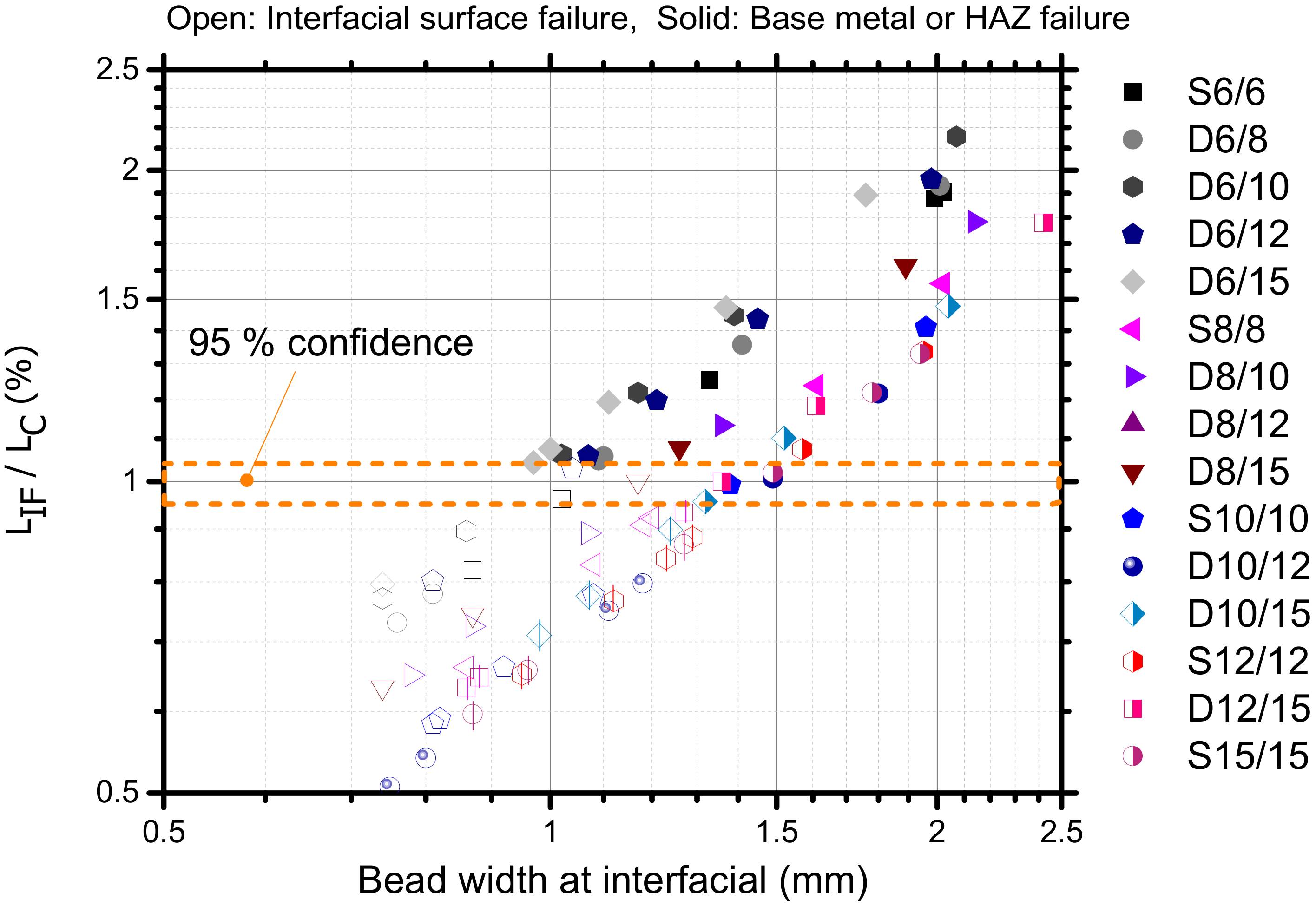
As shown in Figure 10, a comparison between the experiment and estimation was carried out again to evaluate the accuracy of the estimation model. The hollow and solid symbols indicate the IF fracture and the BM of the HAZ fracture, respectively. The failure occurred at the interfacial surface when the ratio was less than 1. The BM and HAZ fracture occurred when the ratio was larger than 1. The fracture mode was perfectly predicted except for the 5% transition region. Even for the 5% transition region, the estimation was incorrect in only three cases. In all cases, if the L_IF value was set only 5% higher than the L_C value, the IF fracture would be avoided.

4. Conclusions

In this study, an analytic model for suggesting an adequate interface bead width was investigated for the laser overlap welding of high-strength steel. The critical interface bead width was defined as the minimum interface bead width required to avoid interface fracturing during a tensile–shear test. An appropriate carbon equivalent formula for a laser-welded high-strength steel was selected, and the hardness profile was predicted. Similar and dissimilar combinations were considered for 590 and 1500 MPa grade steels. The hardness values of the WM and HAZ were predicted with maximum errors of 7.8% and 13.9%, respectively. During the tensile–shear test of high-strength steel, the cosine value of the specimen’s rotation angle was higher than 0.95 at yielding, and the rotation angle was disregarded in the calculation of the shear strength. The critical bead width could be predicted with an accuracy higher than 90%. A model capable of estimating the fracture behavior of the tensile–shear test and suggesting design rules for overlapping welds was successfully developed and evaluated. The model was established based on the chemical composition and tensile strength on the mill sheet supplied by steelmakers. Even without destructive tensile shear tests, a secure welded joint can be achieved by using this simple and analytic model with an additional safety factor of 10% or more.

References

- Lagneborg, R. New steels and steel applications for vehicles. Mater. Des. 1991, 12, 3–14. [Google Scholar] [CrossRef]
- Senuma, T. Physical metallurgy of modern high strength steel sheets. ISIJ Int. 2001, 41, 520–532. [Google Scholar] [CrossRef]
- Takahashi, M. Development of high strength steels for automobiles. Nippon Steel Tech. Rep. 2003, 88, 2–6. [Google Scholar]
- Fan, D.W.; Kim, H.S.; De Cooman, B.C. A review of the physical metallurgy related to the hot press forming of advanced high strength steel. Steel Res. Int. 2009, 80, 241–248. [Google Scholar]
- Karbasian, H.; Tekkaya, A.E. A review on hot stamping. J. Mater. Process. Technol. 2010, 210, 2103–2118. [Google Scholar] [CrossRef]
- Uchihara, M. Joining technologies for automotive steel sheets. Weld. Int. 2011, 25, 249–259. [Google Scholar] [CrossRef]
- Han, T.-K.; Park, B.-G.; Kang, C.-Y. Hardening characteristics of CO2 laser welds in advanced high strength steel. Met. Mater. Int. 2012, 18, 473–479. [Google Scholar] [CrossRef]
- Xia, M.; Biro, E.; Tian, Z.; Zhou, Y.N. Effects of heat input and martensite on HAZ softening in laser welding of dual phase steels. ISIJ Int. 2008, 48, 809–814. [Google Scholar] [CrossRef]
- Mohandas, T.; Reddy, G.M.; Kumar, B.S. Heat-affected zone softening in high-strength low-alloy steels. J. Mater. Process. Technol. 1999, 88, 284–294. [Google Scholar] [CrossRef]
- Biro, E.; McDermid, J.; Embury, J.; Zhou, Y. Softening kinetics in the subcritical heat-affected zone of dual-phase steel welds. Metall. Mater. Trans. A 2010, 41, 2348–2356. [Google Scholar] [CrossRef]
- Kim, C.; Choi, J.-K.; Kang, M.; Park, Y.-D. A study on the CO2 laser welding characteristics of high strength steel up to 1500 MPa for automotive application. J. Achiev. Mater. Manuf. Eng. 2010, 39, 79–86. [Google Scholar]
- Dearden, J.; O’Neill, H. A Guide to the Selection and Welding of Low Alloy Structural Steels; Welding Research Council of the Institute of Welding: Cambridge, UK, 1940. [Google Scholar]
- Ito, Y.; Bessyo, K. Weldability Formula of High Strength Steels: Related to Heat-Affected Zone Cracking; IIW Document IX-567-568; IIW: Warsaw, Poland, 1968. [Google Scholar]
- Yurioka, N.; Suzuki, H. Determination of necessary preheating temperature in steel welding. Weld. J. 1983, 62, 147–153. [Google Scholar]
- Yurioka, N. Physical metallurgy of steel weldability. ISIJ Int. 2001, 41, 566–570. [Google Scholar] [CrossRef]
- Kasuya, T.; Yurioka, N.; Okumura, M. Methods for predicting maximum hardness of heat-affected zone and selecting necessary preheat temperature for steel welding. Nippon Steel Tech. Rep. 1995, 65, 7–14. [Google Scholar]
- Kasuya, T.; Hashiba, Y. Carbon equivalent to assess hardenability of steel and prediction of HAZ hardness distribution. Nippon Steel Tech. Rep. 2007, 95, 53–61. [Google Scholar]
- Kaizu, S.; Shinbo, Y.; Ono, M. Relationship between Vickers hardness of laser weld and chemical composition of steel sheets. Prepr. Natl. Meet. JWS 1994, 55, 118–119. [Google Scholar]
- Taka, T.; Yamamoto, T. The hardness of laser welded metal in steel sheets. In Proceedings of the 34th Material Processing Conference; Japan Laser Processing Society: Osaka, Japan, 1995; pp. 113–122. [Google Scholar]
- Den Uijl, N.J.; Nishibata, H.; Smith, S.; Okada, T.; van der Veldt, T.; Uchihara, M.; Fukui, K. Prediction of post weld hardness of advanced high strength steels for automotive application using a dedicated carbon equivalent number. Weld. World 2008, 52, 18–29. [Google Scholar] [CrossRef]
- Jeon, I.-H.; Kim, C.; Kim, J.-D. Hardness estimation of laser welded boron steel welds with the carbon equivalent. J. Weld. Join. 2016, 34, 1–5. (In Korean) [Google Scholar] [CrossRef]
- Ono, M.; Yoshitake, A.; Ohmura, M. Laser weldability of high-strength steel sheets in fabrication of tailor welded blanks. Weld. Int. 2004, 18, 774–784. [Google Scholar] [CrossRef]
- Miyazaki, Y.; Furusako, S. Tensile shear strength of laser welded lap joints. Nippon Steel Tech. Rep. 2007, 95, 28–34. [Google Scholar]
- Kang, M.; Kim, C.; Lee, J. Weld strength of laser-welded hot-press-forming steel. J. Laser Appl. 2012, 24, 022004. [Google Scholar] [CrossRef]
- Benasciutti, D.; Lanzutti, A.; Rupil, G.; Haeberle, E.F. Microstructural and mechanical characterisation of laser-welded lap joints with linear and circular beads in thin low carbon steel sheets. Mater. Des. 2014, 62, 205–216. [Google Scholar] [CrossRef]
- Furusako, S.; Miyazaki, Y.; Hashimoto, K.; Kobayashi, J. Establishment of a model predicting tensile shear strength and fracture portion of laser-welded lap joints. In Proceedings of the International Congress on Laser Advanced Materials Processing, Osaka, Japan, 27–31 May 2002; pp. 197–202. [Google Scholar]
- Ono, M.; Kabasawa, M.; Omura, M. Static and fatigue strength of laser-welded lap joints in thin steel sheet. Weld. Int. 1997, 11, 462–467. [Google Scholar] [CrossRef]
- Terasaki, T.; Kitamura, T. Prediction of static fracture strength of laser-welded lap joints by numerical analysis. Weld. Int. 2004, 18, 524–530. [Google Scholar] [CrossRef]
- Asim, K.; Lee, J.; Pan, J. Failure mode of laser welds in lap-shear specimens of high strength low alloy (HSLA) steel sheets. Fatigue Fract. Eng. Mater. Struct. 2012, 35, 219–237. [Google Scholar] [CrossRef] [Green Version]
- Lee, J.; Asim, K.; Pan, J. Modeling of failure mode of laser welds in lap-shear specimens of HSLA steel sheets. Eng. Fract. Mech. 2011, 78, 374–396. [Google Scholar] [CrossRef]
- Ha, J.; Huh, H. Failure characterization of laser welds under combined loading conditions. Int. J. Mech. Sci. 2013, 69, 40–58. [Google Scholar] [CrossRef]
- Ma, J.; Kong, F.; Liu, W.; Carlson, B.; Kovacevic, R. Study on the strength and failure modes of laser welded galvanized DP980 steel lap joints. J. Mater. Process. Technol. 2014, 214, 1696–1709. [Google Scholar] [CrossRef]
- Yang, Y.-P.; Cao, Z.; Gould, J.; McGaughy, T.; Jennings, J. Develop an excel-based modeling tool to predict weld and HAZ cooling rate and hardness for pipeline welding. In Proceedings of the ASME 2015 Pressure Vessels and Piping Conference, Boston, MA, USA, 19–23 July 2015. [Google Scholar]
- Miyazaki, Y.; Sakiyama, T.; Kodama, S. Welding techniques for tailored blanks. Nippon Steel Tech. Rep. 2007, 95, 2–10. [Google Scholar]
- Ion, J.; Easterling, K.E.; Ashby, M. A second report on diagrams of microstructure and hardness for heat-affected zones in welds. Acta Metall. 1984, 32, 1949–1962. [Google Scholar] [CrossRef]
- Pavlina, E.; Van Tyne, C. Correlation of yield strength and tensile strength with hardness for steels. J. Mater. Eng. Perform. 2008, 17, 888–893. [Google Scholar] [CrossRef]
Figure 1.
Schematic of prepared specimen to (a) measure the strength and (b) observe the rotation angle during the tensile–shear test.
Figure 2.
Bead width measured at interfacial surface according to welding condition; (a) similar combination; (b) dissimilar combination.
Figure 3.
(a) Measured Vickers hardness profile depending on welding speed: (a) 590 DP; (b) 980 DP.
Figure 4.
Measured hardness of weld metal, heat-affected zone, and base metal.
Figure 5.
Classification of failure mode and effective force to fracture depending on ruptured location at (a) base metal, (b) interfacial surface, and (c) heat-affected zone.
Figure 6.
Digital image correlation (DIC) and high-speed camera images during tensile testing. The observed positions are indicated on the strength–displacement curves of the interfacial surface failure specimen of 590 DP at the (a) initial state, (b) displacement by 0.34 mm, and (c) displacement by 0.39 mm; and the specimen of 1180 CP at the (d) initial state, (e) displacement by 0.69 mm, and (f) displacement by 0.75 mm.
Figure 7.
Tensile stress of base materials at failure and failure location according to bead width at the interfacial surface of (a) similar and (b) dissimilar material joints. The solid symbols indicate the failure location at the base metal or heat-affected zone, and the hollow symbols indicate the interface fracture.
Figure 8.
Comparison of measured and predicted hardness values.
Figure 9.
Calculated critical interface bead width: (a) similar material combination; (b) dissimilar material combination. The error bars indicate the transition region of the failure mode from IF to BM or HAZ during the tensile–shear test.
Figure 10.
Ratio of estimated interface bead width (LIF) to measured interface bead width (LC). The solid symbols indicate the failure location of the base metal or heat-affected zone; the hollow symbols indicate the interfacial failure.