Article

Effects of Chemical Composition and Austenite Deformation on the Onset of Ferrite Formation for Arbitrary Cooling Paths

Materials and Production Technology Department, University of Oulu, 90014 Oulu, Finland
*
Author to whom correspondence should be addressed.
Metals 2018, 8(7), 540; https://doi.org/10.3390/met8070540
Submission received: 5 June 2018 / Revised: 6 July 2018 / Accepted: 10 July 2018 / Published: 12 July 2018
(This article belongs to the Special Issue Advances in Low-carbon and Stainless Steels)

Abstract

:
We present a computational method for calculating the phase transformation start for arbitrary cooling paths and for different steel compositions after thermomechanical treatments. We apply the method to quantitatively estimate how much austenite deformation and how many different alloying elements affect the transformation start at different temperatures. The calculations are done for recrystallized steel as well as strain hardened steel, and the results are compared. The method is parameterized using continuous cooling transformation (CCT) data as an input, and it can be easily adapted for different thermomechanical treatments when corresponding CCT data is available. The analysis can also be used to obtain estimates for the range of values for parameters in more detailed microstructure models.

1. Introduction

Modern thermomechanically processed steels can be rolled and cooled to a variety of microstructures with properties tailored to many kinds of applications. To minimise scatter in microstructures and properties it is beneficial to have phase transformation models that are as accurate as possible. To be able to predict and understand the onset of phase transformations occuring during the complex cooling path of hot rolled steel for different compositions, a quantitative model is needed. To give a realistic estimate, the model should take into account the severe mechanical deformation occurring in hot rolling prior to cooling. In addition, it should be possible to extend the model and adapt it to specific steels and mechanical treatments prior to cooling. It is also desirable that the input data required for the model are easy to obtain, for example, by constant cooling rate experiments.
Several phase transformation models that can be used for simulations along arbitrary cooling paths have been introduced earlier, for example, references [1,2,3,4,5,6,7,8,9,10,11]. However, there is currently no method that includes the effect of austenite deformation on the transformation start for different steel compositions and which could be used to calculate the transformation start for arbitrary cooling path. Since the nucleation phenomenona during the onset of transformation is different from the successive growth stage, several models separate the growth kinetics of the phase transformation from the onset stage by considering an incubation time or delay for the transformation start [3,4,5,7,8,10,11]. However, these models do not consider the effect of deformation prior to cooling [6,7,8,9], or they are specific to a certain steel composition, or they only take in to account the effect of a few alloying elements [2,3,4,5,10,11].
Also, detailed models, such as [12,13,14], which include the description of the steel microstructure, can be used to calculate phase transformation phenomena. These detailed models include a number of parameters which can be either obtained experimentally [13,14] or calculated using theory [12]. Such detailed models could benefit from data that can be obtained directly from linear cooling rate experiments in order to find the range of possible values for the parameters.
The method for calculating the start time of transformation from temperature–time transformation (TTT) diagrams has been presented in several articles, e.g., [1,6,7,8,15], which could be used to calculate the transformation start by applying Scheil’s additivity rule for an arbitrary cooling path. However, it has been shown that using such isothermal transformation data to calculate the transformation start for cooling conditions by applying the additivity rule can give incorrect estimates [16,17]. For cooling, the application of the so-called ideal (or true) incubation time [18,19] gives a better estimate for the transformation start for an arbitrary cooling path [20], as it gives exactly the correct continuous cooling transformation (CCT) diagram for constant cooling rates when Scheil’s additivity principle is applied.
We present a computational method to calculate an estimate for the ferrite phase transformation start of an arbitrary cooling path and for varying steel compositions containing the following alloying elements: C, Si, Mn, Cr, Cu, Ni, Mo, V, Ti, B, and Nb. The model can be easily adapted for new steels and thermomechanical treatments by using constant cooling rate CCT data as the input for the model. The transformation start time includes the time required for the formation of critical-sized nuclei (incubation time) as well as the time required for the growth of the nuclei to the volume fraction required for the detection of the phase transformation start. The method comprises three parts as follows: (1) Calculation of the CCT start time for different steel compositions and phases using the results presented in [21,22] for steels subjected to strain relevant to hot rolling procedures; (2) construction of the so-called ideal TTT diagram [18,19,20,23,24] from a constant cooling rate CCT diagram; and (3) application of Scheil’s additivity principle to calculate the phase transformation start for an arbitrary cooling path after the ideal TTT diagram has been calculated [18]. We show how it is used to quantitatively compare the manner in which different alloying elements affect the austenite to ferrite phase transformation start time and the corresponding activation energy for a given steel composition. The same calculation is done for steel which has been additionally strained below the no-recrystallization temperature, and the results are compared. We also calculate an estimate for the phase transformation start for different kinds of cooling paths.
Since the model presented in this work is based on experimental CCT diagrams [21], it can be easily adapted and extended for different steels when there is a need to obtain more detailed estimates for given steel compositions or mechanical treatments prior to cooling. If constant cooling rate CCT data is analyzed, it can be used as the basis of this method, and the corresponding results, as presented in this article, can be obtained. We separately analyze the austenite to bainite transformation onset and present the results in [25,26].

2. Theory

2.1. Calculation of CCT Start Time for Different Steel Compositions

An estimate for the phase transformation start point in CCT diagrams for different steel compositions can be calculated with Equations (1) and (2) which were presented in reference [21]. As described in the original works, the equations were obtained by linear regression analyses on the effect of alloying elements on the CCT diagrams, considering the following elements: C, Si, Mn, Cr, Cu, Ni, Mo, V, Ti, B, Nb. The experimental results were obtained with 34 different steel compositions by cooling specimens after thermomechanical treatments relevant to industrial hot rolling and cooling processes.
T s , cct ( K ) = 273.15 + B 0 + i B i c i T N + B t arcsinh ( t 85 t 85 , k )
log 10 ( t 85 , k ) = A 0 + i A i c i
where T s , cct ( K ) is the start temperature (in degrees Kelvin) for the phase transformation occurring with a constant cooling rate; c i are the concentrations of different elements in the steel composition in weight %; A i and B i are the constants obtained from the regression analysis; t 85 is the time elapsed while cooling the specimen from 800 C to 500 C; and t 85 , k corresponds to the critical cooling rate, which is the slowest cooling rate that does not produce a measurable phase transformation. T N is used to denote 273 . 15 + B 0 + i B i c i . Prior to cooling, the steel sample was subjected to a mechanical deformation schedule consisting of either (a) two 20% strain deformations above the recrystallization limit temperature, or (b) the same as (a) but with an additional 30% deformation below the non-recrystallization temperature. The different deformation schedules (a and b) yielded different CCT start curves and regression constants. The regression constants for ferrite transformation for both deformation schedules were given in reference [21] and are reproduced in Table 1.
The composition limits (in wt %) for the experimental data used in the regression analysis are shown in Table 2 [21,27].
A comparison with the experimental results showed that the functional form of Equation (1) represents the transformation to ferrite near the critical cooling rate (or t 85 , k ) well. For some steels whose CCT diagrams indicate a transformation start near the equlibrium A e 3 temperature, the functional form gives a slightly higher value for the transformation temperature near the equlibrium temperature than that observed experimentally. When the transformation temperature described by Equation (1) of the steel is well below the equilibrium temperature, the functional form represents the transformation temperatures for the whole experimental range, t 85 t 85 , k 1000 s , well.
At a constant cooling rate, θ ˙ = ( 300 K ) / t 85 , the temperature of the specimen can be expressed as T = A e 3 θ ˙ t , where A e 3 is the equilibrium ferrite formation temperature, and t is the time spent below the A e 3 temperature. By applying Equations (1) and (2), the time required for phase transformation to start during cooling, t s , cct is given by Equation (3):
t s , cct = A e 3 T s , cct 300 t 85 = A e 3 T s , cct 300 sinh T s , cct T N B t + t 85 , k .
Equation (3) is valid for the temperatures where Equations (1) and (2) represent the experimental results well (see discussion above) and can be used to calculate t s , cct for different temperatures, T s , cct . The coordinates ( t s , cct ( T s , cct ) , T s , cct ) then represent the CCT diagram in time-temperature coordinates. Following [28], we used Equation (4) to describe the A e 3 temperature (in degrees Kelvin):
A e 3 ( K ) = ( 1184 29 M n + 70 S i 10 C r ) ( 418 32 M n + 86 S i + 1 C r ) C + 232 C 2
where the element symbols refer to their concentrations (in wt %). The equation includes the effects of C, Mn, Si and Cr. The effect of small amounts of microalloying with other elements is neglected for the equilibrium temperature calculation [28].
The CCT start curve was calculated using Equations (1)–(3) and is shown in Figure 1 with the critical cooling rate, which is the slowest cooling rate that does not produce the phase transformation. The plot was calculated for a steel composition of 0.09 C, 0.28 Si, 1.53 Mn, 0.012 P, 0.005 S, 0.03 Al, 0.05 Cr, 0.05 Cu, 0.035 Nb, 0.04 Ni, 0.02 Ti and 0.05 V (wt %) (named “TH16” in reference [22]) which was subjected to mechanical deformation but allowed time to recrystallize prior to cooling. To describe the “nose” of the CCT diagram without discontinuities in the temperature derivative, a piecewise polynomial was used for smooth transition from the CCT curve to the critical cooling rate curve (see Figure 1).

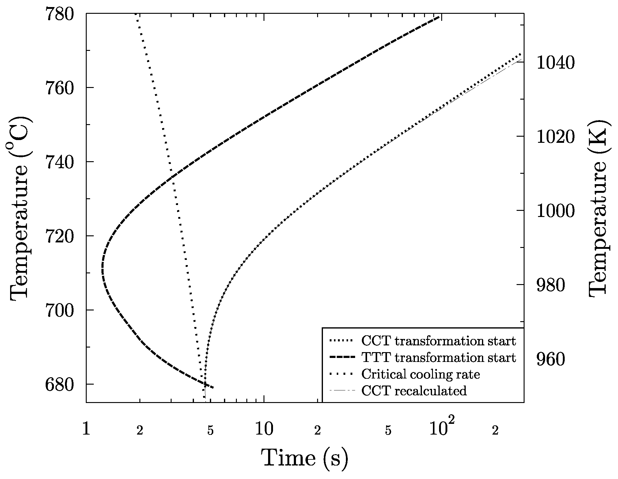
2.2. Construction of the Ideal TTT Diagram from the Constant Cooling Rate CCT Diagram

The ideal isothermal transformation time, τ , can be calculated using Equation (5) [19,29]
1 τ ( Δ T CCT ) = d θ ˙ c ( Δ T CCT ) d Δ T CCT
where the function θ ˙ c ( Δ T ) is the constant cooling rate required to produce a transformation start exactly at the point of undercooling, Δ T CCT (or, equivalently, Δ T CCT is the amount of undercooling at which the transformation starts for constant cooling rate θ ˙ c ). Applying the chain rule of differentiation we obtain
1 τ ( T s , cct ) = d θ ˙ c ( T s , cct ) d T s , cct
where T s , cct is the transformation start temperature in the CCT diagram.

2.2.1. Construction of the Ideal TTT Diagram from ( t 85 ( T s , cct ) , T s , cct ) CCT Diagram

The numerical value of the ideal isothermal start time can be obtained by taking the difference approximation of Equation (6) and solving for τ ( T s , cct ) Δ T s , cct / Δ θ ˙ c ( T s , cct ) , where Δ T s , cct = ( T s , cct + h / 2 ) ( T s , cct h / 2 ) = h and Δ θ ˙ c ( T s , cct ) = θ ˙ c ( T s , cct + h / 2 ) θ ˙ c ( T s , cct h / 2 ) for a sufficiently small h value. The numerical value for the isothermal start time can be calculated using Equations (1), (2) and (7).
τ ( T s , cct ) Δ T s , cct Δ θ ˙ c ( T s , cct ) = h 300 1 t 85 ( T s , cct h / 2 ) 1 t 85 ( T s , cct + h / 2 )
where t 85 ( T s , cct ± h / 2 ) represent the function values of t 85 ( T ) at T = T s , cct ± h / 2 . When the value h = 0.1 K was used, the recalculation of the CCT diagram from the TTT diagram using Equation (12) successfully replicated the original CCT diagram (as shown in Figures 3 and 4).

2.2.2. Construction of the Ideal TTT Diagram from ( t s , cct ( T s , cct ) , T s , cct ) type CCT Diagram

The numerical value of the isothermal start time can also be obtained from the ( t s , cct ( T s , cct ) , T s , cct ) type constant cooling rate CCT diagram, where t s , cct and T s , cct are the time and temperature coordinates of the CCT curve and T start is the cooling start temperature temperature, by using the difference approximation described in Section 2.2.1. Since the constant cooling rate is θ ˙ c = ( T start T s , cct ) / t s , cct ( T s , cct ) , Equation (8) describes the ideal isothermal start time as a function of temperature.
τ ( T s , cct ) Δ T s , cct Δ θ ˙ c ( T s , cct ) = h T start ( T s , cct h / 2 ) t s , cct ( T s , cct h / 2 ) T start ( T s , cct + h / 2 ) t s , cct ( T s , cct + h / 2 )
where t s , cct ( T s , cct ± h / 2 ) represent the function values of t s , cct ( T ) at T = T s , cct ± h / 2 . Equation (8) can be used to calculate the ideal isothermal transformation start, τ ( T ) , when the constant cooling CCT curve ( t s , cct ( T s , cct ) , T s , cct ) is known.

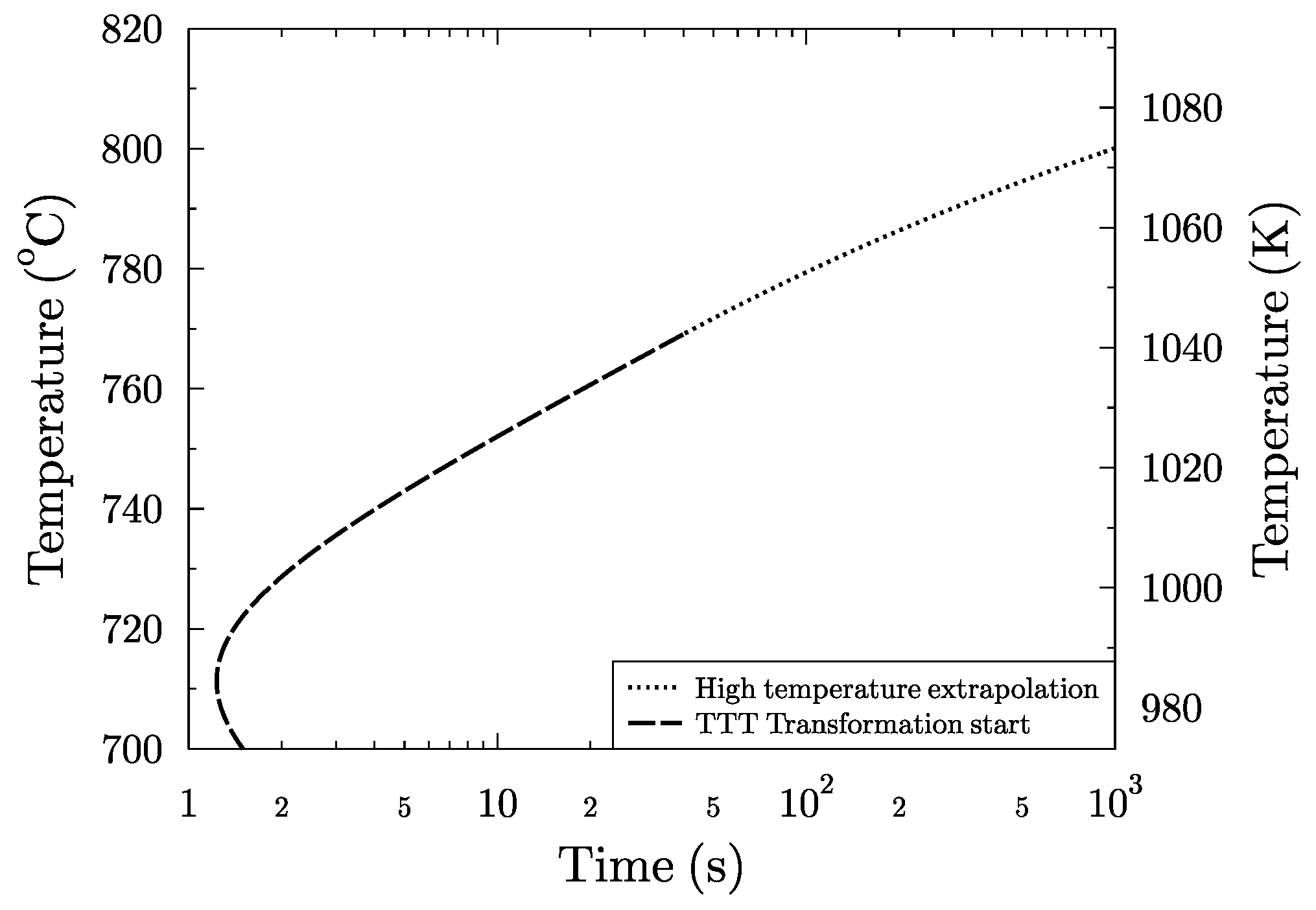
2.2.3. High Temperature Extrapolation of the TTT Start Time

For ferrite formation, we used the following high temperature extrapolation of the calculated ideal TTT start time. The function describing the isothermal transformation start time can be expressed by Equation (9) [20]
τ = K exp ( Q R T ) Δ T m
where K and m are constants; R is the ideal gas constant; T is the absolute temperature; Δ T = A e 3 T is the amount of undercooling; and Q is the activation energy to facilitate carbon mobility in the austenite–ferrite transformation.
Taking the logarithm of both sides of the Equation (9) and differentiating yields,
d ln τ d T = Q R T 2 + m A e 3 T
Since near the equilibrium, A e 3 , the temperature is m A e 3 T > > Q R T 2 , we approximate d ln τ d T m A e 3 T . This allows us to use Equation (11) for high temperature extrapolation of the transformation start time:
ln τ ln B m ln ( A e 3 T ) τ B Δ T m
where the constants B and m are determined from the conditions under which the functions ln τ and d ln τ / d T are continuous. The ideal TTT curve calculated from the CCT diagram as well as the high temperature extrapolation are shown in Figure 2.

2.3. Calculation of the Phase Transformation Start for an Arbitrary Cooling Path

Once the ideal isothermal transformation time has been constructed, it can be used to calculate the transformation start time for an arbitrary cooling path using Scheil’s additivity principle. The transformation is assumed to start when the sum of the fractional transformation times equals one, as shown in Equation (12) [18,19,20,30].
i = 1 n t i τ i ( T ) = 1
where t i is the time spent at temperature T, and τ i ( T ) is the time required to produce a measurable transformation at that temperature.
To check that the computational method gave the correct result, the CCT diagram, which was obtained using the regression Equations (1) and (2), was recalculated using the obtained ideal TTT diagram and Scheil’s additivity principle, as shown in Equation (12). We also compared the results to the experimental data presented in reference [22] for steel “TH16”. The comparison is shown in Figure 3 and Figure 4. The agreement between the original CCT diagram obtained by the regression formulas and the recalculated CCT diagram is excellent. Also, the comparison with the experimental data [22] shows a good agreement, although the difference between the experimental result and the CCT curve calculated with the regression equations is slightly higher for the temperatures near the CCT “nose” for this steel, as shown in the logarithmic plot in the inset of Figure 4. In any case, at temperatures above 993 K (720 C), the experimental values also agree well with the computed values.

2.4. Effective Activation Energy of the Transformation Start

Since ferrite nucleation is a thermally activated process, it can be described using the concept of activation energy [31,32,33,34]. The observed transformation start includes the nucleation of microscopic nuclei as well as the growth of the nuclei to a size at which the transformation can be observed by dilatometric measurement. The transformed fraction, χ , at a constant temperature can be described by an Avrami type Equation (13) [31,32,33]:
χ = 1 exp [ ( k t ) n ] ( k t ) n
where the coefficient k is related to the nucleation and growth rates, and n is related to the shapes of the growing nuclei, and the approximation is valid for a small value of ( k t ) n (i.e., for the start of the transformation) [35]. We emphasize that during the intial stages of the transformation, before it has proceeded to the extent that it can be measured (e.g., 1% transformation), the values for k and n can be different than those produced later in the transformation [16]. This is because the energetically most favourable nucleation sites are consumed early in the process, and the transformed and diffusion regions do not overlap for the first ferrite regions that form on the austenite grain boundaries, whilst the mean carbon content of the austenite increases as the transformation proceeds.
Since both nucleation and growth are thermally activated processes, coefficient k can be described by the Arrhenius type Equation (14) [31,32,33,34]:
k = A exp E A ( T ) R T
where E A ( T ) is the effective activation energy, which depends on the temperature due to effects of undercooling (i.e., thermodynamic driving force) and atomic diffusion; R is the gas constant; A = C ω is a prefactor, which relates to the attempt frequency, ω , and the concentration of heterogenous nucleation sites, C. The effective activation energy is a linear combination of the activation energies of nucleation and growth [31,32,33,34].
By substituting Equation (14) in to Equation (13) and solving for t, we can obtain an expression for the time, τ , required to produce a measurable transformation, χ m , at a given temperature, T, through Equation (15):
τ = K exp E A ( T ) R T
where K = χ m 1 n / A . Since the effective activation energy depends on the temperature, it is not straightforward to obtain its value. However, it is possible to show how different factors affect the transformation start from the differences in transformation start times, as described in Section 3.

3. Results

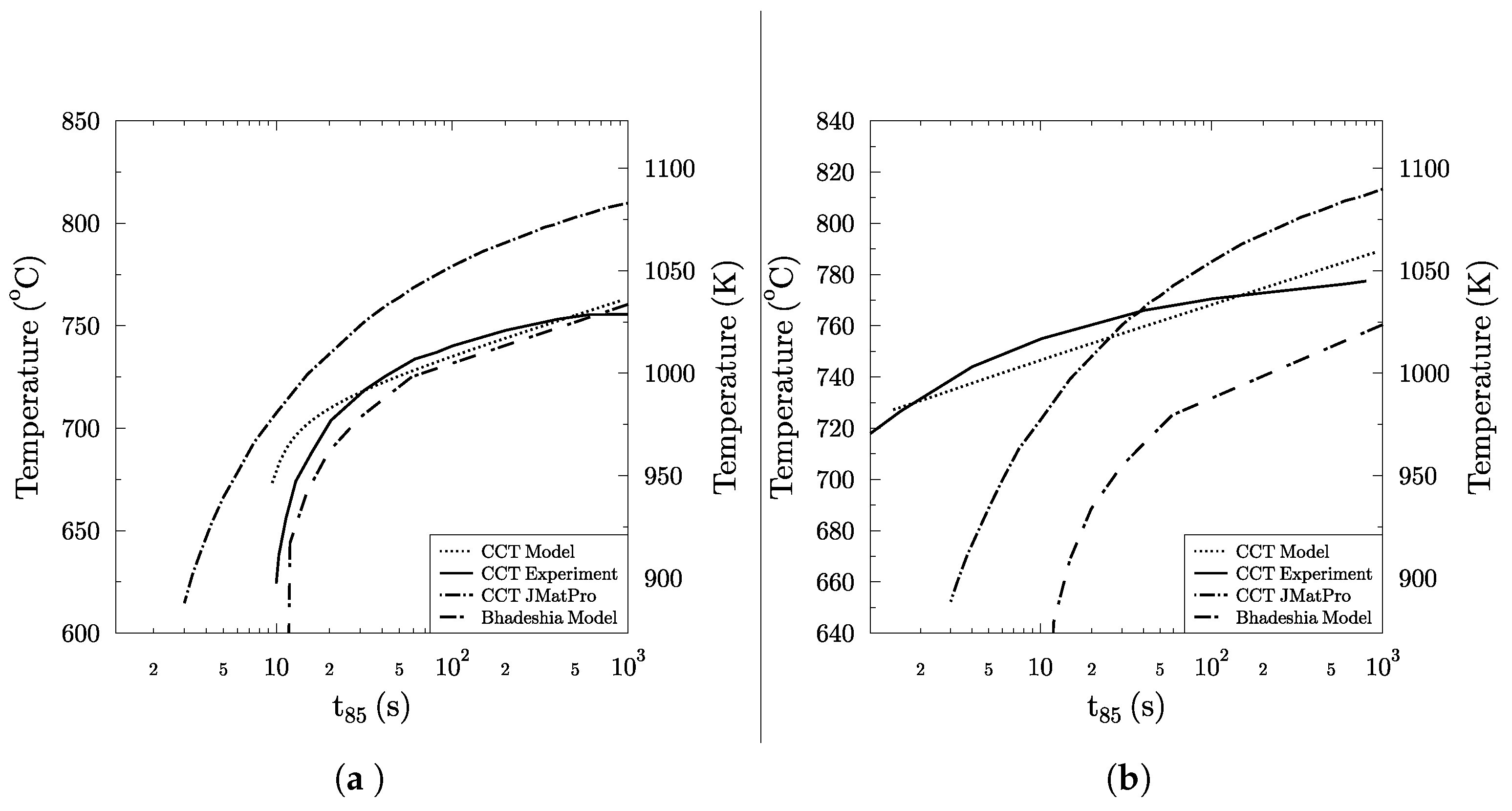
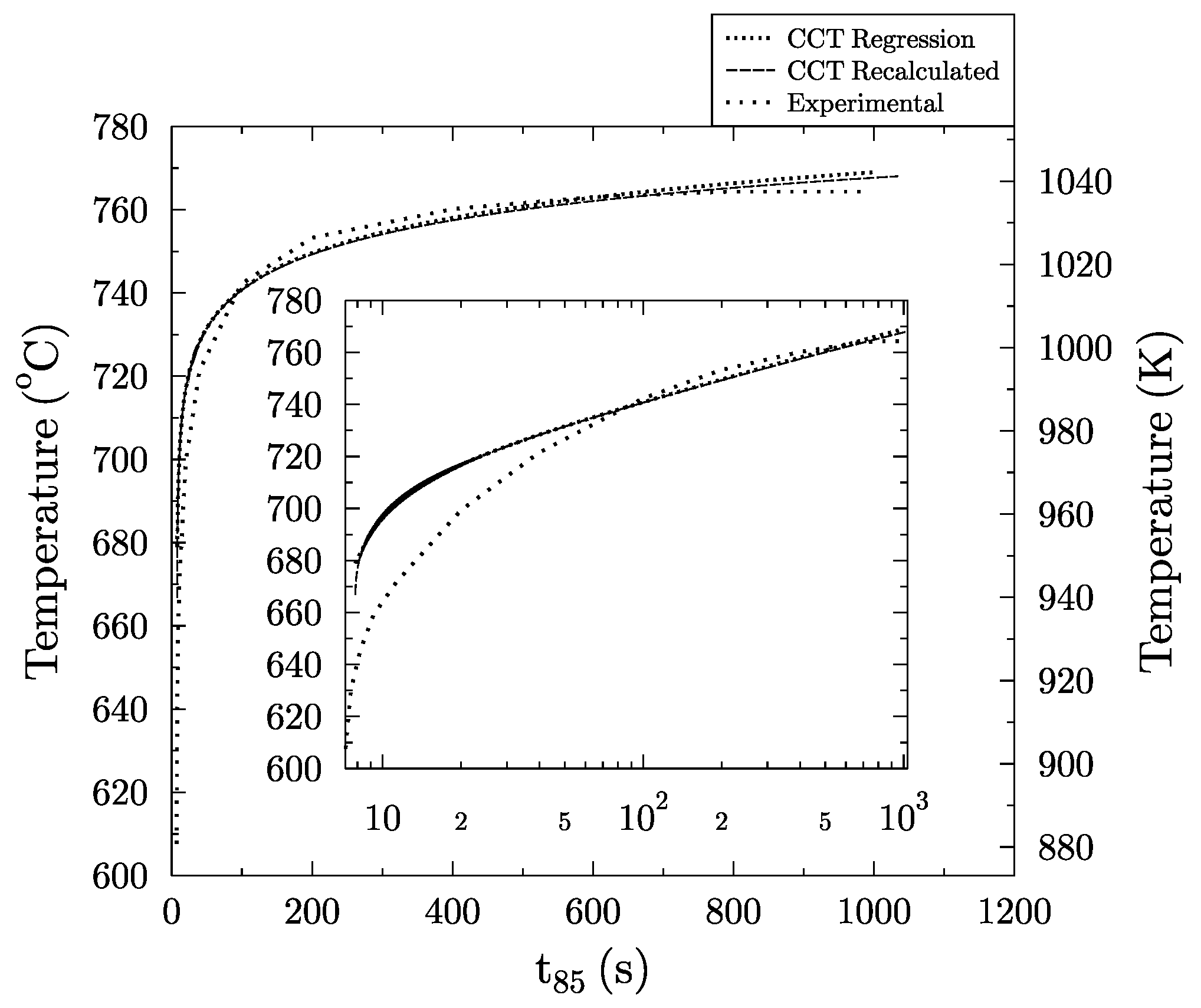
3.1. Model Validation

To demonstrate the benefits of using the model that has been specifically fitted to the experimental CCT data obtained after the thermomechanical processing described earlier, we compared the results obtained with Equations (1) and (2) to the corresponding simulations that were obtained with the commercial software JMatPro (TM) [1] as well as to the simulations based on the model described in [8]. This was possible, since the experimental data presented in the original reference [27] contained information on the austenite grain sizes of several steels, which could be used as input for the JMatPro (TM) software. The phase transformation model of the JMatPro (TM) software is a modified version of the Kirkaldy–Venugopalan phase transformation model [6], and it was fitted to isothermal transformation data [1]. The comparison is shown in Figure 5a,b. Experimentally-measured grain sizes were used as input in the JMatPro simulations. For the fully crystallized case, the DIN grain size number was 6, and for the strain hardened case, the DIN grain size number was 7.
To see how well the model can predict the transformation start for other steels that were not used in the regression fitting, we also compared the model result to CCT diagrams of other steels that were deformed in the austenite state [36]. Although the deformation conditions were not exactly the same as those used in the fitting model, the comparison shows that the model can give reasonable predictions (similar accuracy as in [6]) for the transformation start for some cases. The steel compositions and deformation schedules for these experimental data were as follows: (I) 0.08 C, 1.52 Mn, 0.37 Si, 0.007 S, 0.023 P, 0.21 Cr, 0.10 Ni, 0.10 V, 0.05 Nb, 0.34 Cu, 0.02 Al and 0.008 N (wt %), strained for 0.25 at 1000 C followed by 0.45 strain at 850 C [36]; and (II) 0.10 C, 0.87 Mn, 0.33 Si, 0.24 Mo, 0.002 B, 0.005 N, 0.48 Zr (wt %) strained for 0.25 at 830 C [36,37]. The deformation schedule used in case (I) corresponds that the use of the model fitted to the CCT and most likely for this reason the results had better agreement than in case (II). It must also be mentioned that for one case, the comparison against the experimental CCT data described in reference [36] (page 600, upper diagram) matched poorly. Hence, when using the model to estimate the transformation start for steels that have been subjected to different thermomechanical treatments than the one described earlier, or that have chemical compositions that are much different from the data that was used in the fitting of the regression model [21,27], experimental verification should be performed. In any case, we have demonstrated that the use of the model fitted to the CCT data from exact thermomechanical processing conditions (Figure 5a,b) can give more accurate information on the process than using general transformation formulas that have been obtained by fitting to isothermal transformation data without deformation, as shown in Figure 5.

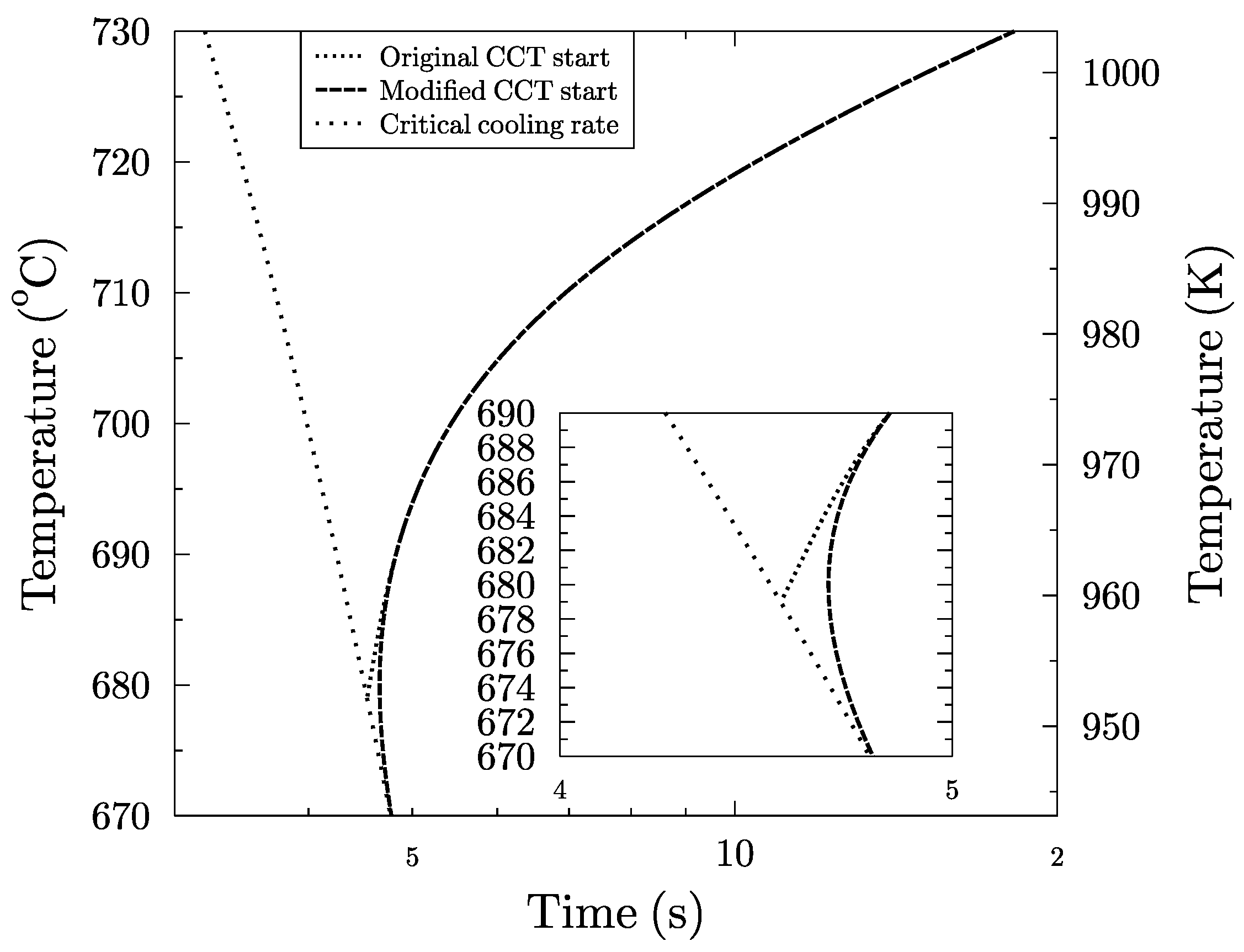
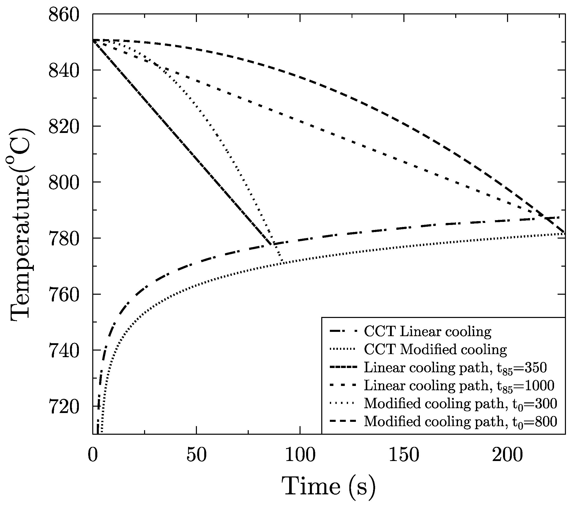
3.2. Phase Transformation Start Calculation for Arbitrary Cooling Path

When the ideal TTT diagram has been determined for a given steel composition, it can be used to calculate the phase transformation start for an arbitrary cooling path. To give an example of this, we calculated transformation start diagrams for two different kinds of cooling paths: (1) for linear cooling paths, T ( t ) = A e 3 θ ˙ t , where the constant cooling rate, θ ˙ , was varied; and (2) for modified cooling paths, T ( t ) = A e 3 ( 1 ( t / t 0 ) 2 ) , where the time constant, t 0 , was varied. The transformation start curves as well as two examples of the cooling paths are shown in Figure 6 for both types of cooling paths.

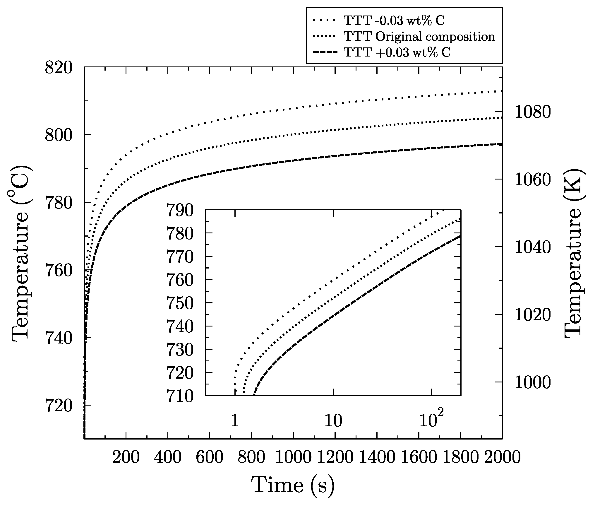
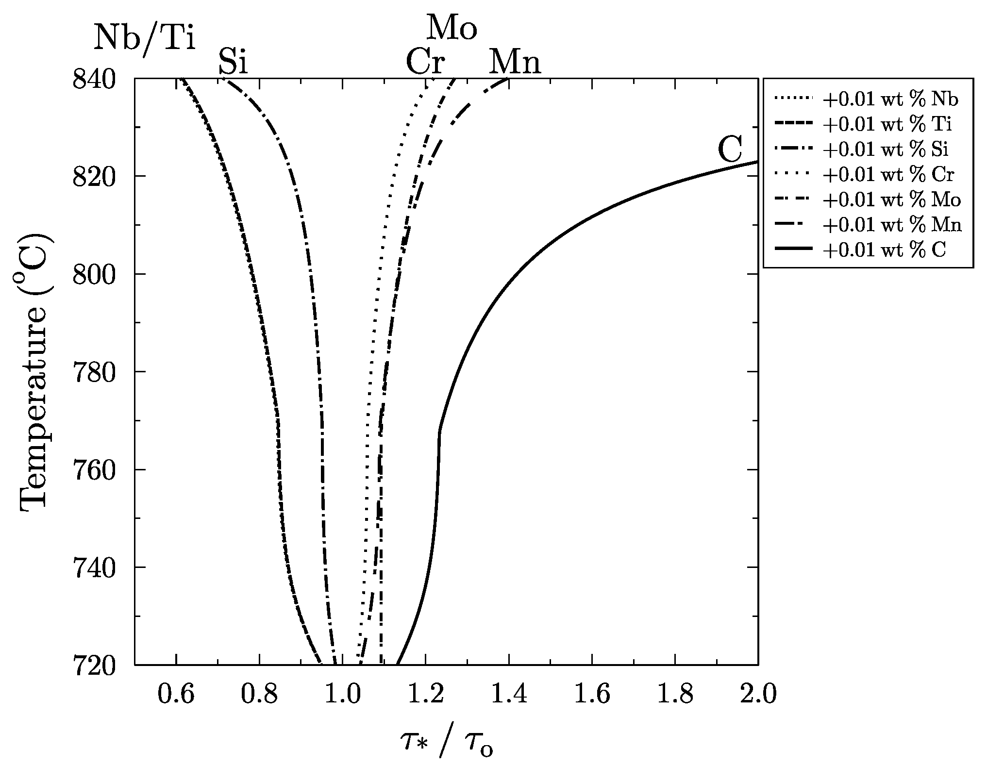
3.3. How Different Alloying Elements Affect the Phase Transformation Start

The alloying elements affect the phase transformation start via two main mechanisms. The chemical composition directly affects the effective activation energy of the transformation. Also, because the chemical composition can affect the grain growth and recovery of dislocation structures after deformation, the chemical composition can also affect the transformation start by changing the concentration of heterogenous nucleation sites. In order to obtain a useful measure which takes into account both of the effects, we analyzed the effect of different elements on the transformation start in the following way. First, the ideal TTT start diagram was calculated for the original steel composition, τ o ( T ) . After this, the concentration of one alloying component was altered and the TTT start diagram was calculated for the altered composition, τ ( T ) . By comparing the original TTT start diagram and the altered TTT start diagram, the extent to which the change in the alloying component affected the TTT start time could be observed. Figure 7 shows how changing the carbon concentration of the steel “TH16” [22] affected the transformation start time. The effect of alloying on the transformation start during constant cooling rate is given by Equations (1) and (2) [21], which formed the basis of our analysis.
Using the previously calculated incubation times τ and τ o , we were able to calculate a useful measure to concisely describe both the effect of chemical composition on the transformation start as well as its effect on the number of nucleation sites. Since the effect of chemical composition on the thermal vibrations of the atoms is negligible, the fraction of the calculated transformation start times, Equation (16), gives a value that can be used to parameterize more detailed microstructure models. However, more information on the effect of chemical composition on the prior austenite microstructure and available nucleation sites is needed.
τ τ o = C o C e x p E A , ( T ) E A , o ( T ) R T
where C and C o are the concentrations of the nucleation sites corresponding to τ and τ o ; and E A , ( T ) and E A , o ( T ) are the effective transformation activation energies at different temperatures. The fractions of the transformation start times for elements that had non-negligible effects on the transformation start in the experimental analysis are shown in Figure 8 [21].

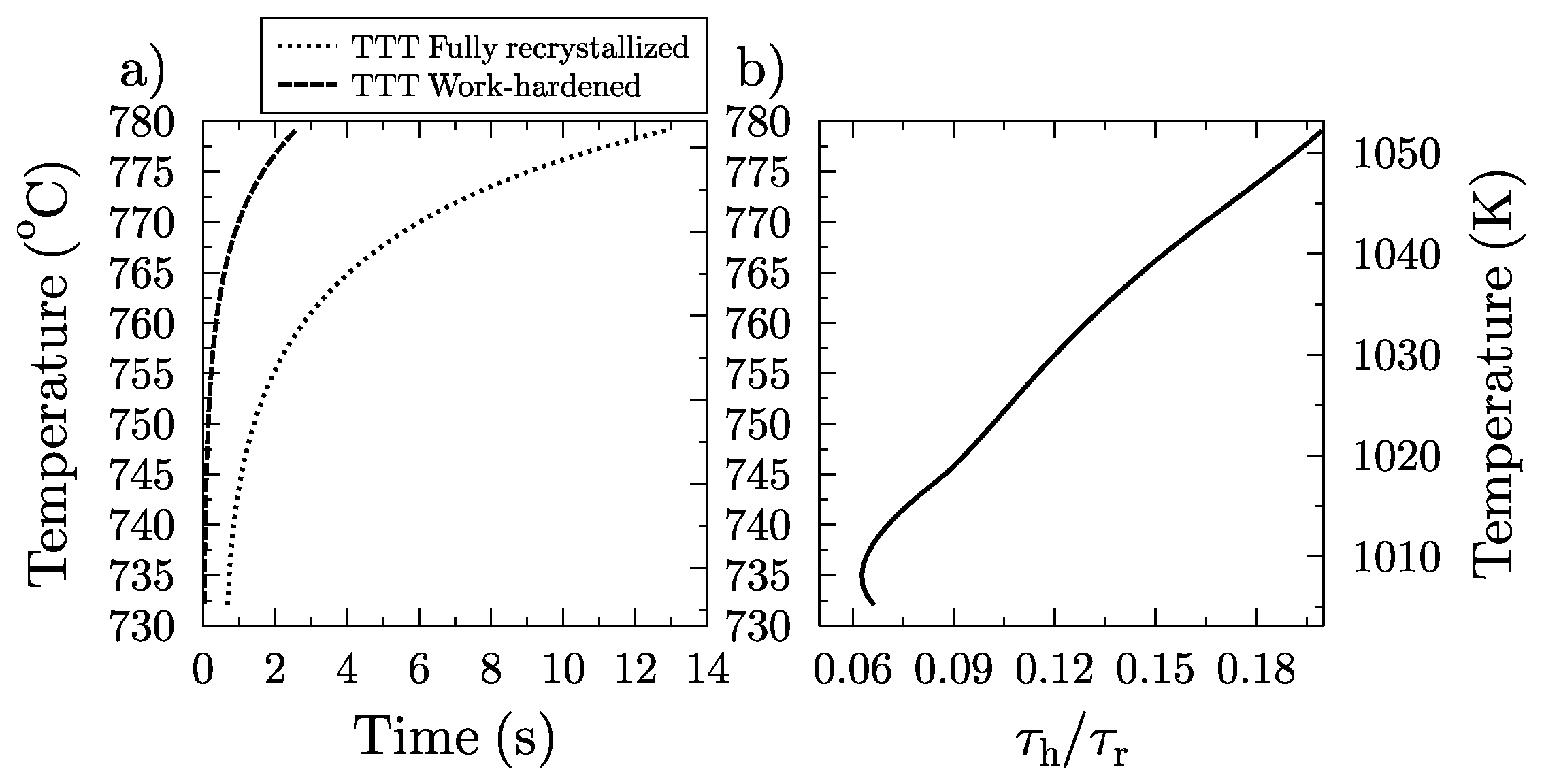
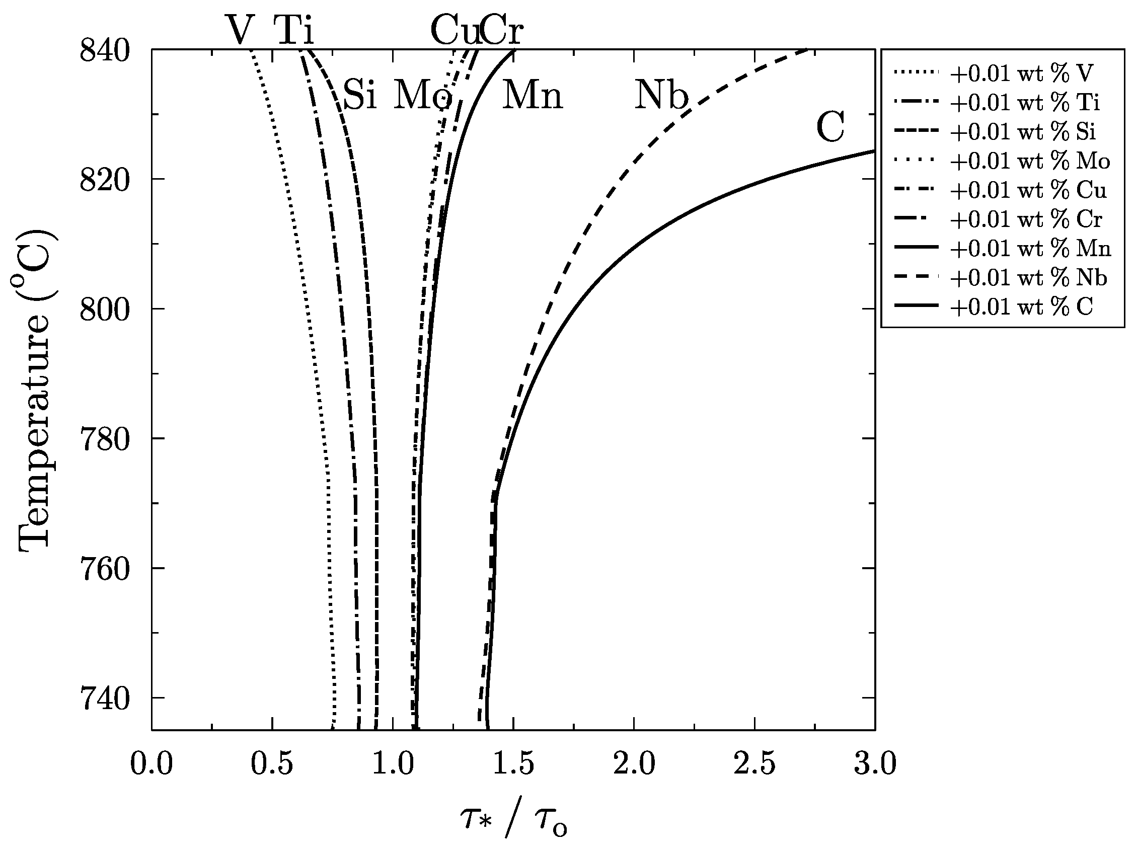
3.4. Effect of Strain Hardening on the Phase Transformation Start

The microstructure of the steel and the phase transformation start are affected by the final rolling temperature and the time spent at elevated temperature prior to cooling. If the steel is rolled above the recrystallization limit temperature and kept at a high temperature prior to cooling, the mechanically-deformed grains have adequate time to recrystallize. In contrast, if the metal is additionally rolled at or below the temperature where no significant recrystallization occurs, the austeninte grains do not have time to recrystallize prior to cooling and are in a more unstable state. This causes the ferrite transformation to start earlier for strain hardened austenite. A comparison of numerical simulation studies to experimental data showed that deformation affects transformation mainly via reduction in the undercooling required for nucleation [38].
The original reference [21] that we used for calculating the transformation start temperatures and critical cooling rates via Equations (1) and (2), also provided the regression constants for strain hardened metal. It is therefore straightforward to calculate the same quantities for the strain hardened steel that were calculated for the fully recrystallized steel. The effects of different alloying elements on the transformation start of the strain hardened material are shown in Figure 9. By comparing the results, we can analyze the effect of strain hardening on the transformation onset.
We calculated the original ideal TTT transformation start time for the fully recrystallized steel, τ r , and the strain hardened steel, τ h , at different temperatures (Figure 10a). To quantitatively analyze the effect of strain hardening versus fully recrystallized steel, we also calculated the fraction τ h / τ r by applying Equation (16). The result is shown in Figure 10b. The steel composition used in the calculation was 0.096 C, 0.150 Si, 1.204 Mn, 0.018 P, 0.006 S, 0.008 N, 0.032 Al, and 0.036 Nb (wt %).

4. Discussion

4.1. Model Validation

The results show that the use of a model that has been fitted to the CCT data from exact thermomechanical processing conditions (Figure 5a,b) gives more accurate results for the process than using general transformation formulas that have been obtained by fitting to isothermal transformation data without prior austenite deformation.

4.2. Phase Transformation Start Calculation for an Arbitrary Cooling Path

In Figure 6, it is clearly shown that for the modified cooling paths where the material spends more time at high temperatures, the transformation start occurs at lower temperatures than for the linear cooling paths. The reason for this is that at higher temperatures, where the undercooling is lower, the driving force for transformation is also lower. This result shows how the method can be quantitatively used to find a desired cooling path to fine-tune the final microstructure by calculating an estimate for the required cooling to achieve transformation start at lower or higher temperatures.

4.3. Effects of Chemical Composition on Transformation Start for Fully Recrystallized Steel

The effects of different alloying elements are qualitatively described in reference [39]. All the alloying elements, including the carbide-forming elements, were in solution at the start of the phase transformation, but following controlled deformation in the no-recrystallization regime, it is possible that some carbide-forming elements tended to promote strain-induced precipitation at some stage. Thermodynamically strain-induced ferrite formation is most likely to precede, or at least compete with, the precipitation process at some point. In any case, the precipitation state after the deformation schedules corresponds more closely to actual rolling conditions than the use of traditional CCT or TTT diagrams, as pointed out in [27]. The following descriptions in [39] agree well with our results and provide a physical explanation for some of the curves. Silicon and niobium promote ferrite formation, while carbon, manganese, chromium, and molybdenum retard the phase transformation. Carbon and manganese are austenite stabilizers. Manganese enhances carbon enrichment by increasing carbon solubility in austenite. Molybdenum exerts an important solute drag effect and delays the transformation of austenite to ferrite and to pearlite strongly. Contrary to its strong carbide forming tendency from a thermodynamic point of view, carbide precipitation is often retarded in presence of molybdenum [39].

4.4. Effects of Chemical Composition on Transformation Start for Strain Hardened Steel

For many alloying elements, the effects on transformation start is similar to those for the fully recrystallized case, but the absolute value of the effect is larger (i.e., the curves are spread wider apart from the zero axis). However, there are a few differences; for example, vanadium, which has a negligible effect for the fully recrystallized steel, promotes ferrite formation for the strain hardened steel. The effect of vanadium in promoting ferrite formation is mentioned in reference [39]. Also, copper, which has a negligible effect for the fully recrystallized steel, retards the transformation of strain hardened steel. Niobium, which promotes ferrite formation for the fully recrystallized material has the opposite effect for the strain hardened material. The effect of niobium in delaying the transformation for the strain hardened material can be explained by reduction of the prior austenite grain boundary energy [40]. After the additional deformation at a lower temperature, the niobium segregates more effectively to the grain boundaries than after high temperature deformation [35]. The reduction in the austenite grain boundary energy lowers the energy gain associated with ferrite nucleation on grain boundaries [40] and delays the nucleation. Niobium may also behave in a manner similar to molybdenum because of comparable atomic diameters and due to its ability to exert a strong solute drag pressure despite its carbide-forming tendency. However, this requires confirmation experiments with high resolution TEM studies to identify any possible precipitation.
According to the regression constants shown in Table 1 [21,27], boron should have almost negligible effect on transformation start. Since the study [27] was not specifically designed to show the effect of boron, this result may be misleading and has not been included in Figure 8 and Figure 9. However, the regression constants fitted to describe the hardness of the steel after cooling in the same study [27] show that boron has a significant hardening effect on steel subjected to deformation schedule (b). The conclusion from [27], therefore, is that, for strain hardened steel, boron operates by reducing the increase in the ferrite volume fraction with time during cooling rather than through its effect on the start point of the transformation.

5. Conclusions

A computational model which can be used to analyze the onset of phase transformation for different steel compositions following different thermomechanical treatments prior to cooling was presented. The model can calculate the transformation start temperature for an arbitrary cooling path, and it can be used to analyze the effects of different alloying elements and mechanical straining on the transformation start at different temperatures. The calculation of transformation start for an arbitrary cooling path is of practical importance as it can be used in the design of cooling schedules. The estimate for the extent to which different alloying elements affect the phase transformation onset gives some indications of the underlying processes. These indications can be helpful in the construction of more detailed microstructure models, especially in finding ranges for different parameters in such models. Our computational method can be easily parameterized using constant cooling rate CCT data. When more detailed data is needed, for example, to consider the effect of different mechanical treatments prior to cooling, the method presented in this article can also be used.

Author Contributions

Methodology and Software A.P.; Writing—Original Draft Preparation, A.P.; Writing—Review & Editing, M.S., D.P.; Project Administration and Funding Acquisition, D.P.

Funding

This research was funded by TEKES through Finnish Metals and Engineering Competence Cluster (FIMECC) System Integrated Metals Processing (SIMP) Showcase 2.2 program as well as Digital Internet Materials & Engineering Co-Creation (DIMECC) Flex project.

Conflicts of Interest

The authors declare no conflict of interest. The founding sponsors had no role in the design of the study; in the collection, analyses, or interpretation of data; in the writing of the manuscript, and in the decision to publish the results.

Nomenclature

T s , cct Start temperature for the phase transformation occurring with a constant cooling rate.
c i The concentrations of different elements in the steel composition in weight %.
t 85 The time elapsed while cooling the specimen from 800 C to 500 C.
t 85 , k The t 85 time corresponding to the slowest cooling rate that does not produce phase transformation.
A i Constant obtained from the regression analysis.
B i Constant obtained from the regression analysis.
T N 273.15 + B 0 + i B i c i .
θ ˙ Cooling rate.
A e 3 Equilibrium ferrite formation temperature.
ttime.
t s , cct Time required for phase transformation to start during cooling.
τ Ideal isothermal transformation time.
CCTContinuous cooling transformation.
TTTTime–temperature transformation.
Δ T Undercooling, i.e., the temperature below A e 3 temperature.
θ ˙ c ( Δ T ) Constant cooling rate required to produce transformation start at undercooling Δ T .
T s , cct Transformation start temperature in the CCT diagram.
hValue used in difference approximation.
KConstant used in describing ideal TTT start time.
mConstant used in describing ideal TTT start time.
RIdeal gas constant.
QActivation energy.
BConstant used in high temperature extrapolation of ideal TTT start time.
t i Isothermal timestep used in the application of Scheil’s rule.

References

  1. Saunders, N.; Guo, Z.; Li, X.; Miodownik, A.; Schillé, J.P. The Calculation of TTT and CCT Diagrams for General Steels. JMatPro Softw. Literat. 2004. Available online: http://www.thermotech.co.uk/resources/TTT_CCT_Steels.pdf (accessed on 11 July 2018).
  2. Kwon, O. A technology for the prediction and control of microstructural changes and mechanical properties in steel. ISIJ Int. 1992, 32, 350–358. [Google Scholar] [CrossRef]
  3. Chen, X.; Xiao, N.; Li, D.; Li, G.; Sun, G. The finite element analysis of austenite decomposition during continuous cooling in 22MnB5 steel. Model. Simul. Mater. Sci. Eng. 2014, 22, 065005. [Google Scholar] [CrossRef]
  4. Wang, X.; Li, F.; Yang, Q.; He, A. FEM analysis for residual stress prediction in hot rolled steel strip during the run-out table cooling. Appl. Math. Model. 2013, 37, 586–609. [Google Scholar] [CrossRef]
  5. Woodard, P.; Chandrasekar, S.; Yang, H. Analysis of temperature and microstructure in the quenching of steel cylinders. Metall. Mater. Trans. B 1999, 30, 815–822. [Google Scholar] [CrossRef]
  6. Kirkaldy, J.S.; Venugopalan, D. Prediction of microstructure and hardenability in low alloy steels. In Proceedings of the International Conference on Phase Transformations in Ferrous Alloys, Philadelphia, PA, USA, 4–6 October 1983; Marder, A.R., Goldstein, J.I., Eds.; Metallurgical Society of AIME: Warrendale, PA, USA, 1983; pp. 125–148. [Google Scholar]
  7. Lee, J.; Bhadeshia, H. A Methodology for the Prediction of Time-Temperature Transformation Diagrams. Mater. Sci. Eng. A-Struct. 1993, 171, 223–230. [Google Scholar] [CrossRef]
  8. Bhadeshia, H. Thermodynamic Analysis of Isothermal Transformation Diagrams. Met. Sci. 1982, 16, 159–165. [Google Scholar] [CrossRef]
  9. Li, M.; Niebuhr, D.; Meekisho, L.; Atteridge, D. A computational model for the prediction of steel hardenability. Metall. Mater. Trans. B 1998, 29, 661–672. [Google Scholar] [CrossRef]
  10. Fernandes, F.; Denis, S.; Simon, A. Mathematical model coupling phase transformation and temperature evolution during quenching of steels. Mater. Sci. Technol. 1985, 1, 838–844. [Google Scholar] [CrossRef]
  11. Pandi, R.; Militzer, M.; Hawbolt, E.; Meadowcroft, T. Modelling of austenite decomposition kinetics in steels during run-out table cooling. In Proceedings of the International Symposium on Phase Transformations During the Thermal/Mechanical Processing of Steel; Hawbolt, E.B., Yue, S., Eds.; Canadian Institute of Mining, Metallurgy and Petroleum: Vancouver, BC, Canada, 1995; pp. 459–471. [Google Scholar]
  12. Umemoto, M.; Hiramatsu, A.; Moriya, A.; Watanabe, T.; Nanba, S.; Nakajima, N.; Anan, G.; Higo, Y. Computer modeling of phase transformation from work-hardened austenite. ISIJ Int. 1992, 32, 306–315. [Google Scholar] [CrossRef]
  13. Enomoto, M.; Yang, J.B. Simulation of nucleation of proeutectoid ferrite at austenite grain boundaries during continuous cooling. Metall. Mater. Trans. A 2008, 39, 994–1002. [Google Scholar] [CrossRef]
  14. Militzer, M.; Pandi, R.; Hawbolt, E. Ferrite nucleation and growth during continuous cooling. Metall. Mater. Trans. A 1996, 27, 1547–1556. [Google Scholar] [CrossRef]
  15. Enomoto, M. Prediction of TTT-Diagram of Proeutectoid Ferrite Reaction in Iron Alloys from Diffusion Growth Theory. ISIJ Int. 1992, 32, 297–305. [Google Scholar] [CrossRef]
  16. Hawbolot, E.; Chau, B.; Brimacombe, J. Kinetics of Austenite-Pearlite Transformation in Eutectoid Carbon Steel. Metall. Trans. A 1983, 14, 1803–1815. [Google Scholar] [CrossRef]
  17. Zhu, Y.; Lowe, T. Application of, and precautions for the use of, the rule of additivity in phase transformation. Metall. Mater. Trans. B 2000, 31, 675–682. [Google Scholar] [CrossRef]
  18. Wierszyllowski, I. The effect of the thermal path to reach isothermal temperature on transformation kinetics. Metall. Mater. Trans. A 1991, 22, 993–999. [Google Scholar] [CrossRef]
  19. Pham, T.; Hawbolt, E.; Brimacombe, J. Predicting the onset of transformation under noncontinuous cooling conditions 1. Theory. Metall. Mater. Trans. A 1995, 26, 1987–1992. [Google Scholar] [CrossRef]
  20. Pham, T.; Hawbolt, E.; Brimacombe, J. Predicting the onset of transformation under noncontinuous cooling conditions: Part 2. Application to the austenite pearlite transformation. Metall. Mater. Trans. A 1995, 26, 1993–2000. [Google Scholar] [CrossRef]
  21. Herman, J.-C.; Thomas, B.; Lotter, U. Computer Assisted Modelling of Metallurgical Aspects of Hot Deformation and Transformation of Steels; Publications Office for the European Union: Luxembourg, 1997; pp. 63–64. [Google Scholar]
  22. Herman, J.-C.; Donnay, B.; Schmitz, A.; Lotter, U.; Grossterlinden, R. Computer Assisted Modelling of Metallurgical Aspects of Hot Deformation and Transformation of Steels (Phase 2); Publications Office for the European Union: Luxembourg, 1999; pp. 15, 72–73. [Google Scholar]
  23. Wierszyllowski, I. Discussion of “predicting the onset of transformation under noncontinuous cooling conditions: Part I. Theory and predicting the onset of transformation under noncontinuous cooling conditions: Part II. Application to the austenite pearlite transformation”. Metall. Mater. Trans. A 1997, 28, 251. [Google Scholar] [CrossRef]
  24. Pham, T.; Hawbolt, E.; Brimacombe, J. Authors’ reply. Metall. Mater. Trans. A 1997, 28, 1089. [Google Scholar] [CrossRef]
  25. Pohjonen, A.; Somani, M.; Pyykkönen, J.; Paananen, J.; Porter, D. The onset of the austenite to bainite phase transformation for different cooling paths and steel compositions. Key Eng. Mater. 2016, 716, 368–375. [Google Scholar] [CrossRef]
  26. Pohjonen, A.; Kaijalainen, A.; Somani, M.; Larkiola, J. Analysis of Bainite Onset During Cooling Following Prior Deformation at Different Temperatures. Comput. Methods Mater. Sci. 2017, 17, 30–35. [Google Scholar]
  27. Lotter, U. Aufstellung von Regressionsgleichungen zur Beschreibung des Umwandlungsverhaltens Beim Thermomechanische Walzen, Abslussbericht, Kommission der Europäischen Gemeninschaften, Generaldirektion Wissenschaft, Forshcung und Entwicklung; EUR 13620 DE; Publications Office for the European Union: Luxembourg, 1991; p. 17. [Google Scholar]
  28. Donnay, B.; Herman, J.; Leroy, V.; Lotter, U.; Grossterlinden, R.; Pircher, H. Microstructure Evolution of C-Mn Steels in the Hot Deformation Process: The Stripcam Model. In Proceedings of the 2nd International Conference on Modeling of Metal Rolling Processes, London, UK, 9–11 December 1996; Beynon, J.H., Ingham, P., Teichert, H., Waterson, K., Eds.; Institute of Materials: Cambridge, UK, 1996. [Google Scholar]
  29. Kirkaldy, J.; Sharma, R. A New Phenomenology for IT and CCT Curves. Scr. Metall. Mater. 1982, 16, 1193–1198. [Google Scholar] [CrossRef]
  30. Scheil, E. Anlaufzeit der austenitumwandlung. Arch. Eisenhuttenwes. 1935, 8, 565–567. [Google Scholar] [CrossRef]
  31. Farjas, J.; Roura, P. Modification of the Kolmogorov–Johnson–Mehl–Avrami rate equation for non-isothermal experiments and its analytical solution. Acta Mater. 2006, 54, 5573–5579. [Google Scholar] [CrossRef] [Green Version]
  32. Christian, J. Chapter 12-Formal Theory of Transformation Kinetics. In The Theory of Transformations in Metals and Alloys; Christian, J., Ed.; Pergamon: Oxford, UK, 2002; pp. 529–552. [Google Scholar]
  33. Mittemeijer, E. Fundamentals of Materials Science; Springer Science & Business Media: Berlin/Heidelberg, Germany, 2010. [Google Scholar]
  34. Liu, F.; Sommer, F.; Bos, C.; Mittemeijer, E.J. Analysis of solid state phase transformation kinetics: models and recipes. Int. Mater. Rev. 2007, 52, 193–212. [Google Scholar] [CrossRef]
  35. Porter, D.; Easterling, K.E.; Sherif, M.Y. Phase Transformations in Metals and Alloys; CRC Press: Boca Raton, FL, USA, 2009. [Google Scholar]
  36. Vander Voort, G.F. Atlas of Time-Temperature Diagrams for Irons and Steels; ASM International: Almere, The Netherlands, 1991. [Google Scholar]
  37. Smith, Y.E.; Siebert, C.A. Continuous cooling transformation kinetics of thermomechanically worked low-carbon austenite. Metall. Trans. 1971, 2, 1711–1725. [Google Scholar]
  38. Hanlon, D.; Sietsma, J.; van der Zwaag, S. The effect of plastic deformation of austenite on the kinetics of subsequent ferrite formation. ISIJ Int. 2001, 41, 1028–1036. [Google Scholar] [CrossRef]
  39. Bleck, W. Using the TRIP effect—The dawn of a promising group of cold formable steels. In Proceedings of the International Conference on TRIP-Aided High Strength Ferrous Alloys; De Cooman, B., Ed.; Wissenschaftsverlag Mainz GmbH: Aachen, Germany, 2002; pp. 13–23. [Google Scholar]
  40. Yan, P.; Bhadeshia, H.K.D.H. Austenite-ferrite transformation in enhanced niobium, low carbon steel. Mater. Sci. Technol. 2015, 31, 1066–1076. [Google Scholar] [CrossRef]
Figure 1. The continuous cooling transformation (CCT) diagram for the given steel composition can be calculated with the parameters reported in [21]. To describe the CCT “nose” without discontinuities in the derivative, a spline was fitted between the calculated CCT curve and the critical cooling rate.
Metals 08 00540 g001
Figure 2. The high temperature extrapolation of the ideal temperature–time transformation (TTT curve), calculated using Equation (11), shown together with the ideal TTT start diagram calculated directly from the experimentally fitted CCT curve using Equation (8).
Metals 08 00540 g002
Figure 3. Ideal (or true) isothermal transformation diagram calculated with Equation (8), the original CCT diagram calculated with Equation (3), and the CCT diagram which was recalculated by applying the Scheil’s additivity principle in Equation (12).
Metals 08 00540 g003
Figure 4. To validate the model, the CCT diagram was recalculated from the ideal (or true) TTT curve using Scheil’s additivity rule. The result shows excellent agreement between the original CCT curve calculated from Equations (1) and (2) and the recalculated CCT curve. The results were also compared to the experimental data given in [22]. Note that the original CCT curve and the recalculated curve almost overlap.
Metals 08 00540 g004
Figure 5. (a) CCT start temperature as a function of t 85 calculated with Equations (1) and (2), JMatPro (TM) and the Bhadeshia model [8] and compared against the experimental data presented in reference [27] (steel TH15, 0.11 C, 0.36 Si, 1.57 Mn, 0.018 P, 0.006 S, 0.006 N, 0.038 Al, 0.04 Cr, 0.03 Cu, 0.03 Ni, 0.08 V, 0.045 Nb) for (a) fully recrystallized steel and (b) strain hardened steel. The experimentally-measured grain sizes were used as input in the JMatPro simulations.
Metals 08 00540 g005
Figure 6. Phase transformation start calculated for two different types of cooling paths: (1) the linear cooling paths exemplified by linear plots and (2) the modified cooling paths given by the Equation T ( t ) = A e 3 ( 1 ( t / t 0 ) 2 ) shown by the curved plots.
Metals 08 00540 g006
Figure 7. The start time of the original steel composition is compared to the compositions where the carbon wt % decreased/increased by 0.03%. The inset shows the change on a smaller scale near the ideal TTT “nose” in a logarithmic plot.
Metals 08 00540 g007
Figure 8. The effects of altering different alloying elements on the phase transformation start at different temperatures for fully recrystallized steel (deformation schedule a) is shown by calculating the fraction τ / τ o (see text). The plots were calculated from the difference in the ideal TTT start times for steel “TH16” shown in reference [22] (0.09 C, 0.28 Si, 1.53 Mn, 0.012 P, 0.005 S, 0.03 Al, 0.05 Cr, 0.05 Cu, 0.035 Nb, 0.04 Ni, 0.02 Ti, and 0.05 V wt %).
Metals 08 00540 g008
Figure 9. The effects of altering different alloying elements to the phase transformation start at different temperatures for strain hardened steel (deformation schedule b) is shown by calculating the fraction τ / τ o (see text). The plots are calculated from the difference in the ideal TTT start times for steel “TH16” shown in reference [22] (0.09 C, 0.28 Si, 1.53 Mn, 0.012 P, 0.005 S, 0.03 Al, 0.05 Cr, 0.05 Cu, 0.035 Nb, 0.04 Ni, 0.02 Ti, and 0.05 V wt %).
Metals 08 00540 g009
Figure 10. Comparison of the calculated ideal TTT curves of work hardened versus fully recrystallized austenite: (a) plots of the TTT curves; (b) the time required to start the transformation for strain hardened material divided by the corresponding time for fully recrystallized material.
Metals 08 00540 g010
Table 1. The regression constants given in [21], which were used in Equations (1) and (2). The constants are given for two different deformation schedules, (a) and (b) (see text).
B 0 B C B Si B Mn B Cr B Cu B Mo B V B Ti B B B Nb B t
(a)834.8−25160.5−103.2−69.70−105.502029.020511.86
(b)884.2−33165.2−98.7−75.9−97.4−76.72901580−3229.28
A 0 A C A Si A Mn A Cr A Cu A Mo A V A Ti A B A Nb A Ni
(a)−0.5243.0700.7180.88503.82500000
(b)−0.3193.45−1.4701.44004.22100000
Table 2. The composition limits (in wt %) of the model.
CSiMnPSNAlCr
min0.010.010.160.0070.0020.0030.0020.01
max0.650.711.690.0220.0110.0120.0621.20
CuNiMoVTiBNb
min0000000
max0.301.320.510.100.030.00220.05

