Extension of Experimentally Assembled Processing Maps of 10CrMo9-10 Steel via a Predicted Dataset and the Influence on Overall Informative Possibilities

Abstract

Processing maps embody a supportive tool for the optimization of hot forming processes. In the present work, based on the dynamic material model, the processing maps of 10CrMo9-10 low-alloy steel were assembled with the use of two flow curve datasets. The first one was obtained on the basis of uniaxial hot compression tests in a temperature range of 1073–1523 K and a strain rate range of 0.1–100 s⁻¹. This experimental dataset was subsequently approximated by means of an artificial neural network approach. Based on this approximation, the second dataset was calculated. An important finding was that the additional dataset contributed significantly to improving the informative ability of the assembled processing maps in terms of revealing potentially inappropriate forming conditions.

1. Introduction

Since the end of the 20th century, processing maps, i.e., power dissipation maps superimposed by flow instability maps, have been extensively studied as a very convenient tool for the optimization of hot forming processes, such as rolling, forging, etc. [1,2,3,4,5,6,7,8,9,10,11,12,13,14,15,16,17,18]. These maps simply display the combinations of thermomechanical conditions, i.e., strain, strain rate, and deformation temperature, which are suitable for the forming processes of an examined material. At the same time, they also define the conditions that are less appropriate or even entirely inappropriate [3,13]. In the last two decades, processing maps have been utilized for the study of various materials. For instance, Łyszkowski and Bystrzycki [3] assembled processing maps of an Fe₃Al intermetallic alloy. Quan et al. [4] utilized processing maps to find the optimal working parameters of as-extruded 42CrMo high-strength steel. Gao et al. [5] utilized processing maps to study the hot-working behavior of high-carbon/low-carbon steel composites. Liu et al. [18] were able to create processing maps for an Fe-11Mn-10Al-0.9C duplex low-density steel susceptible to κ-carbides. Saxena et al. [6] compiled power dissipation and flow instability maps of a Zr-2.5Nb zirconium alloy, while Duan et al. [14] developed processing maps for a Pb-Mg-10Al-0.5B alloy. Various other steels and alloys have also been studied on the basis of processing maps, e.g., austenitic heat-resistant stainless steel (Zhou et al. [7]), Ni-based superalloy (Zhang et al. [9]), Cu–Cr–Zr–Nd alloy (Zhang et al. [11]), NiTiNb shape memory alloy (Wang at al. [15]), nanoalumina composite (Suresh et al. [8]), etc. Sonnek and Petruželka [2] created power dissipation and flow instability maps of R7 HSLA steel. They subsequently implemented these maps into a finite element method (FEM) simulation of rail wheel forging.

In the case of materials intended for use in forming, processing maps are assembled on the basis of flow curve datasets, where each flow curve embodies the flow stress development of the studied material under specific thermomechanical conditions [19]. Such datasets are usually obtained by means of torsion or uniaxial compression testing, which is performed in the supposed interval of thermomechanical forming conditions. However, for the creation of processing maps of a TC21 titanium alloy, Zhang et al. [17] were also able to utilize a tensile test dataset. Quan et al. [13] further suggested that a limited number of tested combinations may be the reason for the inferior informative ability of compiled processing maps as compilations are based on datapoint interpolation. For this reason, they proposed to expand an experimental dataset with a set of flow curves predicted at nonexperimental conditions. They utilized this approach in the case of as-extruded 7075 aluminum alloy.

Approximation and subsequent prediction of an experimental flow curve dataset can be performed via derived flow stress models (an index of different models can be found in [20]). Nevertheless, in recent times, this approximation issue has often been solved utilizing artificial neural networks (ANNs), which allow a higher curve fit accuracy [13,19,21,22,23,24]. The ANN approach is part of a wide family of biology-inspired mathematical techniques that are intended to solve complicated scientific and engineering tasks, e.g., highly nonlinear approximation issues [25]. These mathematical approaches have been found to be very useful in various applications (see e.g., [26,27,28]).

In the present work, the processing maps of 10CrMo9-10 low-alloy steel were assembled by combining two flow curve datasets. The first one was obtained on the basis of uniaxial hot compression tests, while the second one was the result of approximation and prediction via a well-adapted multilayer feed-forward artificial neural network. The main aim of this research was to evaluate the influence of the additional (predicted) flow curve dataset on improving the informative possibilities of the compiled processing maps. The research was mainly aimed at the detection of potentially unstable regions, which point to possibly aggravated forming conditions.

2. Materials and Methods

2.1. Experimental Procedure

Samples of the investigated 10CrMo9-10 low-alloy steel (

Table 1. Chemical composition of the investigated 10CrMo9-10 steel in wt %.

C	Cr	Mo	Mn	Si
0.092	2.1	0.93	0.5	0.24

) were taken from the columnar crystal area of a continuously casted bloom (cross Section 205 mm) parallelly to the casting direction. Cylindrical hot compression test samples with a diameter of 10 mm and a height of 15 mm were then prepared by cutting and turning. The prepared samples were subsequently subjected to a uniaxial hot compression testing on a HDS-20 hot deformation simulator (Dynamic Systems Inc., Poestenkill, NY, USA) with the Hydrawedge II testing module (Gleeble system [29]). The tests were carried out at deformation temperature levels of 1073, 1223, 1373, and 1523 K and strain rate levels of 0.1, 1, 10, and 100 s⁻¹ when the value of true (logarithmic) height strain was reaching up to 1.0. Each sample was heated by means of direct electric resistance heating directly up to the deformation temperature with a heating rate of 5 K·s⁻¹, then followed a dwell time of 180 s. The temperature was controlled by a pair of thermocouple wires of K-type, i.e., Ni–Cr (+) and Ni–Al (−), which were welded to the surface of the tested samples in their middle length. The testing procedure was run under vacuum in order to eliminate oxidation processes. This was achieved via a rotary and diffusion pump. Tantalum foils and nickel-based grease were applied in order to reduce friction on the anvils–sample interface. The described testing procedure resulted in a set of 16 experimental flow curves.

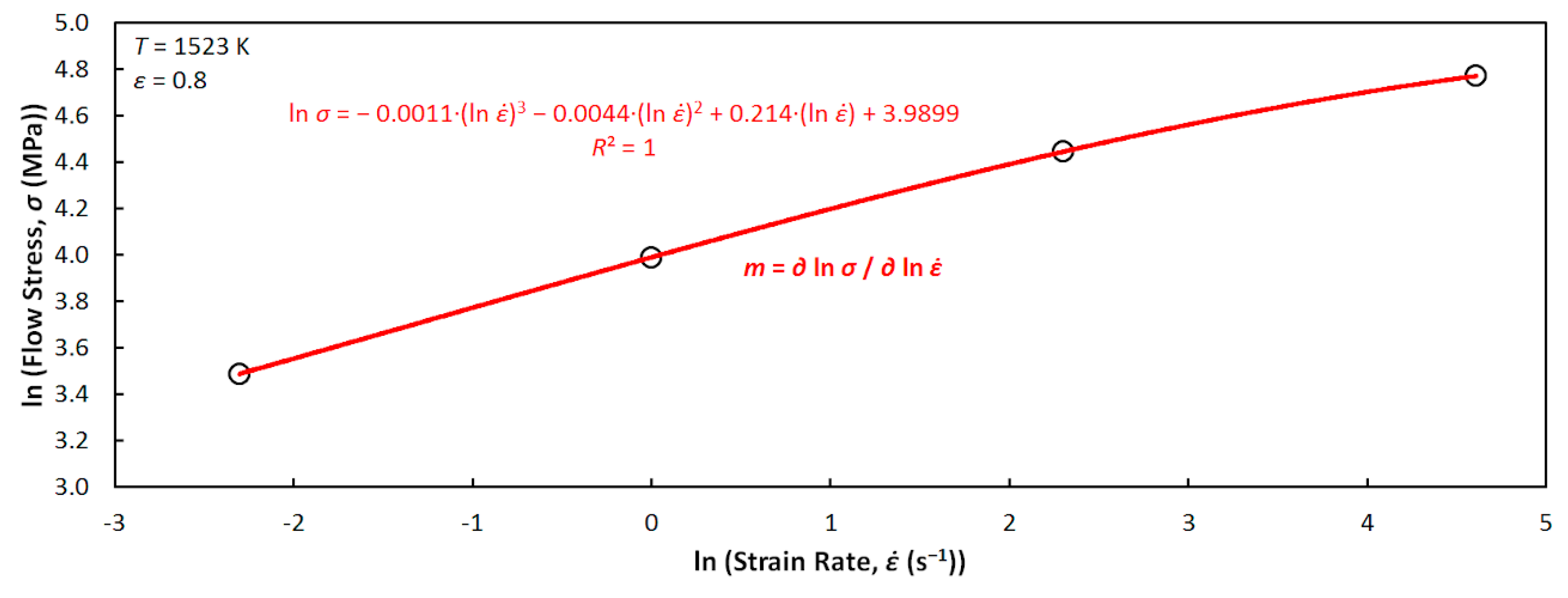
2.2. Approximation of the Experimental Flow Curve Dataset

The experimentally obtained flow curve datasets were approximated and subsequently extended on the basis of prediction at three nonexperimentally tested temperature levels—1148, 1298, and 1448 K—for each tested strain rate (i.e., 12 additional curves were assembled).

The approximation procedure was performed utilizing an ANN approach [30,31,32]. The possibility of approximating experimentally obtained flow curve datasets via AAN has been studied many times as a suitable substitute for the commonly used flow stress models. Various ANN methodologies have been proposed, and studies have been performed on different steels and alloys. All these works have proven that ANN approaches have a positive influence on the accuracy of flow curve dataset approximation, and it is therefore appropriate to use them [13,19,21,22,23,24].

In order to approximate the experimental flow curve dataset of the examined steel, a multilayer feed-forward ANN was assembled, as shown in the general scheme in Figure 1. The vectors of the independent variables were connected with the vector of the dependent variable via a multilayer network of artificial neurons. Neurons of the hidden and output layers represented the main computational units [32]. Each of these neurons was characterized by a weighted sum, Σ, which was transferred into the neuron output, a, via a specific transfer function, f [33]. The neuron communication was mediated via synaptic weights, w. The w-values and the bias values, b, simply represented the material constants of the ANN model. A detailed mathematical description of the utilized ANN is available in [32].

In order to determine a proper ANN architecture, i.e., appropriate number of hidden layers, hidden neurons, and suitable transfer functions, the adaptation procedure was applied. During this process, various network architectures were tested with regard to the approximation accuracy of the experimental dataset and the response ability beyond the experimental conditions (i.e., prediction capability). The tested architectures were always trained to obtain the optimal set of w and b values, i.e., to minimize a mean squared error [34], MSE (MPa²) [13]:

$$\underset{w,b}{\min } MSE=\frac{1}{n}\cdot {\displaystyle {\sum }_{i=1}^n{\left(r_i\right)}^2}$$

(1)

where the value of r_i (MPa) corresponds to the i-th residuum of the network output with i = [1, n] ⊂ ℕ; n is the number of involved datapoints. Based on previous experiences [19], the minimization procedure was performed via the Levenberg–Marquardt algorithm [35,36,37] in combination with Bayesian regularization [38,39] and the use of back-propagation of error signal to the neurons of the hidden layers [40]. For the purpose of network training, the experimental dataset was divided into three parts: training set (containing the datapoints subjected to minimization algorithm), validation set (intended to verify the prediction capability during network training), and testing set (to test the prediction accuracy after the training procedure). The validation set (1373 K/0.1 s⁻¹, 1223 K/10 s⁻¹, and 1073 K/1 s⁻¹, i.e., 151 datapoints) and the testing set (1523 K/1 s⁻¹, 1223 K/100 s⁻¹, and 1073 K/10 s⁻¹, i.e., 150 datapoints) were utilized for the purpose of this research. The rest of the experimental dataset (i.e., 500 datapoints) then served as the training set. Each input vector was normalized as follows [41]:

$$p_{i,norm}=\frac{p_i-\mu }{s}$$

(2)

where p_i and p_i,norm correspond to the i-th un-normalized and normalized value of the input vector, respectively, with i = [1, n] ⊂ ℕ; n is the total number of vector elements. The variables μ and s represent the mean value [42] and the sample standard deviation [43] of the training part of the un-normalized input vector, respectively [41]:

$$\mu =\frac{1}{m}\cdot {\displaystyle {\sum }_{i=1}^m{p}_i}$$

(3)

$$s=\sqrt{\frac{1}{m-1}\cdot {\displaystyle {\sum }_{i=1}^m{\left(p_i-\mu \right)}^2}}$$

(4)

where i = [1, m] ⊂ ℕ; m is the number of vector elements corresponding to the training set. Note that the vector of the network output was not normalized (it was not necessary since there is only one vector in the output layer).

Figure 2 shows how the various architectural settings influenced the network performance (Equation (1)). With respect to the number of hidden layers, the use of two and three layers provided practical and meaningful results, as demonstrated in Figure 2. On the other hand, utilizing only one layer resulted in high MSE values, log(MSE) > 4. In addition, these MSE values remained practically unchanged (constant) despite the various number of neurons. It was obvious that the number of neurons in the hidden layers played a substantial role with regard to network performance. With respect to the training and validation set, similar trends were observed despite the number of hidden layers and the types of transfer functions utilized (the MSE values practically decreased with increasing number of neurons). A certain similarity could also be observed when studying the behavior of the testing set. In the case of two hidden layers, the MSE values of the testing set increased when the number of neurons exceeded the values of 6 and 5 with regard to the hyperbolic tangent sigmoid (tansig) (Figure 2a) and logistic sigmoid (logsig) (Figure 2b) transfer functions, respectively. This suggests that the network had become overtrained. With respect to the three hidden layers, the MSE values of the testing set pointed to network overtraining, even at a lower number of hidden neurons. In addition, these test MSE values are higher than in the case of two hidden layers.

Based on the training, cross-validation, and testing of various network settings (see Figure 2), the optimal ANN architecture was chosen as follows: two hidden layers, both with six neurons; hyperbolic tangent sigmoid transfer function in the case of each hidden neuron; and pure line function for the neuron of the output layer.

The artificial neural network was created and practically applied in the MATLAB^® R2017b environment [44] using embedded Neural Network Toolbox^TM (see detailed user’s guide in [45]), with the overall processing time taking approximately two working days.

2.3. Assembly of Processing Maps

In the present research, processing maps of the examined low-alloy steel were assembled on the basis of a well-known dynamic material model (DMM) [46,47,48]. In accordance with DMM theory, a hot-formed workpiece (i.e., a workpiece undergoing thermoplastic deformation) is considered as the nonlinear power dissipator. An instantaneous power per unit volume, P (J), is then introduced to represent a physical quantity of power dissipation. This quantity is the sum of two complementary parts: a G content (J) and a J co-content (J) (see detailed analysis in [46]).

The G content is considered to correspond to the power dissipated as a consequence of plastic deformation, which is linked to the temperature increase of the formed material. The J co-content then represents the power associated with metallurgical processes, such as dynamic recovery (DRV), dynamic recrystallization (DRX), etc. [2,5,10]. Variations in the J co-content with the process parameters were applied in order to model the dynamic behavior of the formed material.

The J co-content for common hot-formed engineering materials ranges between two extremes (zero and ideal (maximal) energy dissipation). The ratio between the real and ideal dissipation, known as the efficiency of power dissipation, η, can therefore be utilized to help map the microstructural characteristics of the formed material in a wide range of thermomechanical conditions [2,46]:

$$\eta =\frac{J}{J_{\max }}=\frac{2\cdot m}{m+1}.$$

(5)

The well-known strain rate sensitivity index, m, can be expressed as follows [46]:

$$m={\frac{\partial J}{\partial G}=\frac{\partial \ln \sigma }{\partial \ln \dot{\epsilon }}|}_{T,\epsilon }.$$

(6)

Relevant σ–$\stackrel{.}{\epsilon }$ datapoints were extracted from the experimental and calculated flow curve datasets. In order to perform the derivation, the ln σ vs. ln $\stackrel{.}{\epsilon }$ datapoints were subsequently interpolated by a cubic spline [4], as shown in Figure 3.

A graphical expression of the efficiency of power dissipation, i.e., Equation (5), in relation to the temperature and strain rate at specific strains represented the first part of the processing maps, known as power dissipation maps [2,5]. These maps disclose different areas associated with specific metallurgical processes, where each process is linked to a specific η-range. For instance, the DRX course is usually associated with the η-range of ca. 30–50%, while the lower values can be assigned to the DRV development. Higher η-values (ca. above the 60%) are then commonly attributed to the superplastic behavior [1,2,6].

The second part of the processing maps was given by flow instability maps. These maps have the capability to reveal instability domains, i.e., the areas of less favored or inappropriate thermomechanical conditions. These metallurgical instabilities can be associated with, for example, shear bands, Lüders’ bands, kink bands, or mechanical twinning [2]. The metallurgical instability was determined on the basis of the following continuum criterion [49,50]:

$$\xi \left(\dot{\epsilon }\right)=\frac{\partial \ln \left(\frac{m}{m+1}\right)}{\partial \ln \dot{\epsilon }}+m\le 0$$

(7)

where the variable ξ($\stackrel{.}{\epsilon }$) represents the flow instability parameter. A graphical expression of this parameter with respect to the temperature and strain rate at specific strains embodied the mentioned second part of the processing maps (flow instability maps).

The processing maps were created by superimposing both the abovementioned parts (i.e., flow instability maps over the power dissipation maps) [4]. Processing maps of the investigated steel were graphically expressed by means of the Gnuplot 5.0 Patchlevel 4 [51].

3. Results and Discussion

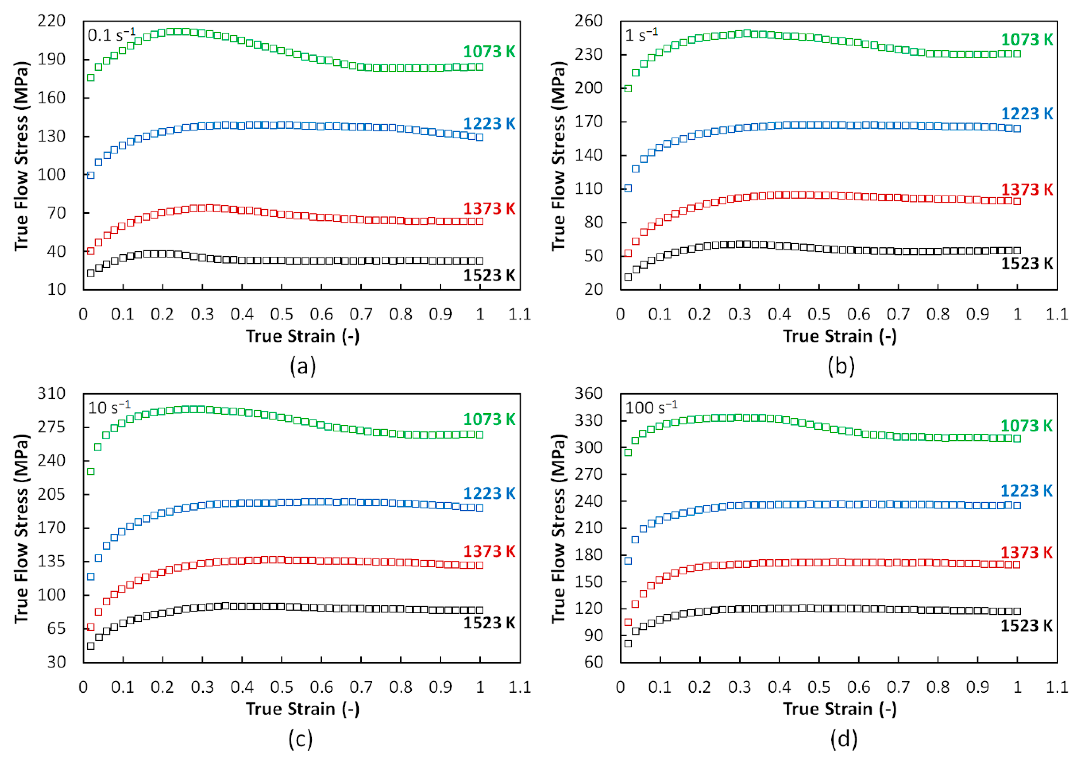
3.1. Experimental Flow Curve Dataset

Figure 4 displays the experimental flow curve dataset, consisting of 16 curves, of the investigated steel. As can be seen, higher temperature in combination with lower strain rate contributed to a decrease in the flow stress level.

As can be seen, the flow curves had two courses. The first one involved a gradual flow stress growth up to the peak point (global maximum) and subsequent steady-state flow (constant phase). This is typical of lower temperatures and higher strain rates. The second one consisted of a decrease in flow stress after the peak point with gradual transition to the steady-state flow. This second course is typical of higher temperatures and lower strain rates. Nevertheless, in the current case, an atypical behavior was also observed. The lowest temperature level (i.e., 1073 K) did not follow the presumed trend. In contrast to other temperature levels, which were linked to the austenitic area, the temperature level of 1073 K corresponded to the ferritic area. This ferritic matrix was probably during the compression transformed to austenite matrix because of the recalescence in the middle part of the tested samples. This might have been the reason for the observed atypical flow curve behavior.

3.2. Calculated Flow Curve Dataset

Figure 5 shows a graphical comparison of the experimental (boxes) and the ANN-approximated (lines) flow curves of the investigated steel. The gray lines represent the curves predicted beyond the experimental temperature levels. As can be seen, the approximation accuracy was high, and even the predicted curves fit into the presumed flow stress levels.

The approximation accuracy was further statistically confirmed by the favorable value of Pearson’s correlation coefficient [52], R (Equation (8) [13]), and also by the average absolute relative error, AARE (%) (Equation (9) [13]), as graphically demonstrated in Figure 6.

$$R=\frac{{\displaystyle {\sum }_{i=1}^n\left[E_i-\mu \left(E\right)\right]}\cdot \left[A_i-\mu \left(A\right)\right]}{\sqrt{{\displaystyle {\sum }_{i=1}^n{\left[E_i-\mu \left(E\right)\right]}^2}\cdot {\displaystyle {\sum }_{i=1}^n{\left[A_i-\mu \left(A\right)\right]}^2}}},$$

(8)

$$AARE=\frac{1}{n}\cdot {\displaystyle {\sum }_{i=1}^n\left|\frac{E_i-A_i}{E_i}\right|\cdot 100}.$$

(9)

In Equations (8) and (9), E_i (MPa) and A_i (MPa) correspond to the experimental and approximated flow stress values, where i = [1, n] ⊂ ℕ; n is the overall number of approximated flow curve datapoints. The μ(E) (MPa) and μ(A) (MPa) then represent the mean value of vectors E and A, respectively.

3.3. Processing Maps

Figure 7 shows the processing maps of the investigated 10CrMo9-10 steel assembled on the basis of the abovementioned methodology. Note that the experimental and ANN data were combined to assemble these maps. In the figure, the black-labeled contours reflect the power dissipation efficiency (η, Equation (5)) in percentage. The instability areas (i.e., ξ-values ≤ 0, Equation (7)), which were calculated on the basis of the experimental dataset, are bounded by the blue (dash–dot–dot) lines. The instability areas of the ANN-based dataset are given by the red (dash) lines.

3.3.1. Instability Areas

Two perspicuous experimental-based instability areas were clearly visible at the strain of 0.2, as shown in Figure 7a:

• The first one (I) was revealed at higher strain rates and lower temperatures. This instability domain, however, gradually vanished with increasing strain. Nevertheless, the ANN dataset enabled instability in this area to be detected at the strain of 0.4, as shown in Figure 7b, and even at higher strain.
• The second one (II) was situated at the lowest strain rates and slightly higher temperature levels. This second region was also visible at the strain of 0.4. In both cases (strains of 0.2 and 0.4), the experimentally revealed low strain rate instability area (II) was significantly enlarged by the ANN-based data. This enlargement was observed towards to lower and higher temperatures and even to higher strain rates. It is evident from Figure 7c,d that the experimentally determined second region occupied a much larger area at the strains of 0.6 and 0.8. Enlargement of this area with ANN-based data is less significant than in the case of lower strains (i.e., 0.2 and 0.4).

Other instability areas could also be observed:

• A small oval instability area (III) was revealed on the basis of the experimental data at the strain of 0.4. This separated region was situated just below the temperature of 1373 K and around the strain rate of 1 s⁻¹. Area III then grew with increasing strain and became a part of area II at the strain of 0.8. However, area III that was detected by the ANN dataset still remained separated from the ANN area II.
• Another new, small instability region (IV) was observed at the strains of 0.6 and 0.8 (1448–1523 K and 10–100 s⁻¹ in Figure 7c,d).

It is understandable that the best forming conditions was at the highest temperatures in combination with the lowest strain rates. No instability was detected at these conditions (see bottom right corner of each map). This fact has been demonstrated in many previously published papers on various materials, e.g.,

• intermetallic alloy [3],
• high-carbon/low-carbon steel composite [5],
• zirconium alloy [6],
• aluminum alloy [13],
• Pb-based alloy [14],
• titanium alloy [17], and
• duplex low-density steel susceptible to κ-carbides [18].

Processing maps in these papers contained various number of instability domains with different sizes and shapes under various thermomechanical conditions. However, the common feature was that no instability region was detected at the highest temperatures and lowest strain rates.

Based on the presented results, it can be said that the additional (ANN) flow curve dataset had a considerable influence in revealing the instability regions (mainly at the strains of 0.2 and 0.4), which can positively contribute to the proper settings of forming conditions. For example, increased awareness about instability occurrence can be utilized for identifying thermomechanical conditions that should be further checked by other methods (e.g., metallographic analyses).

3.3.2. Power Dissipation Efficiency

As can be seen, the η-values exceeded the 30% threshold. This fact indicates that, in the case of the studied steel, DRX took place as a softening mechanism [1,2]:

• The η-values gradually increased with increasing temperature and decreasing strain rate, i.e., the increase in the η-values was closely linked to the softening progress.
• The η-values above 30% were mainly linked to the highest temperatures and lowest strain rates. Of course, the area of η-values higher than 30% also expanded with the increase in strain level into the areas of lower temperatures and higher strain rates, but this expansion was quite limited. The fact is that larger parts of the processing maps remained under the 30% level, which suggests that, for the studied steel, the DRX process needed higher strain levels to be initialized.

The above-described observations can be confirmed by the flow curve courses (see Figure 5). In some cases, the flow stress increased up to the maximum very slowly and only started to visibly fall at the highest strain levels. For example, in Figure 5a, it can be seen that the beginning of the flow stress decrease corresponds to the strain of 0.8 for the flow curve of 1223 K at 0.1 s⁻¹. The softening process in this case was underdeveloped, which was reflected by the low η-values of approximately 20% (see Figure 7d at 1223 K and 0.1 s⁻¹).

The more developed softening process (i.e., η-values above 30%) corresponded to the flow curves that showed quicker initialization of flow stress decrease. This can be seen, for example, in the curves for 1523, 1448, and 1373 K at 0.1 s⁻¹ in Figure 5a and the corresponding η-values, e.g., at the strain of 0.6 (Figure 7c):

• It can be seen that, even when the flow stress decrease was under the conditions initialized at lower strains, the corresponding peak points were quite indistinct, i.e., flow stress decrease was not intensive.
• In fact, flow curves under some other conditions showed rather dynamic recovery behavior (i.e., constant phase after the maximum stress), which was linked to the lower η-values.
• Nevertheless, an exception existed at the temperature level of 1073 K. These curves corresponded to the intensive softening course but without any reflection on the processing maps. In fact, the η-values were even lower at this temperature. This can be attributed to the above-discussed issue (see Section 3.1) dealing with the transformation of ferritic matrix to austenite due to deformation heating. The lower η-values can then be attributed to the aggravated forming conditions that were revealed by the presented instability areas.

4. Conclusions

Processing maps, i.e., power dissipation maps superimposed by the corresponding maps of flow instability, of the 10CrMo9-10 low-alloy steel were assembled on the basis of Prasad’s dynamic material model with the use of two hot flow curve datasets.

An experimental dataset was obtained via a series of 16 uniaxial hot compression tests that were performed at four temperatures (1073, 1223, 1373, and 1523 K) and four strain rates (0.1, 1, 10, and 100 s⁻¹).

An artificial neural network dataset was additionally employed in order to improve the informative ability of the processing maps. This dataset contained approximated experimental curves and curves that were predicted at three additional temperature levels (1148, 1298, and 1448 K) in combination with the abovementioned strain rates. The approximation and subsequent prediction were performed utilizing a multilayer feed-forward ANN. A network-adaptation procedure was realized via the back-propagation of error signal and the Levenberg–Marquardt optimization algorithm together with Bayesian regularization.

The processing maps revealed several instability domains, i.e., areas of less-appropriate forming conditions. It was found that the additional ANN flow curve dataset significantly contributed to the completeness of the processing maps in terms of revealing potentially unstable regions. In other words, the experimental dataset itself does not have to be sufficient for revealing all possibly aggravated forming conditions. The enhanced informative ability of processing maps can be helpful, such as when using other tools to determine proper forming settings, for instance, during the selection of thermomechanical conditions that should be checked by metallographic analyses.

References

1. Chakravartty, J.K.; Prasad, Y.V.R.K.; Asundi, M.K. Processing Map for Hot Working of Alpha-Zirconium. Metall. Trans. A 1991, 22A, 829–836. [Google Scholar] [CrossRef]
2. Sonnek, P.; Petruželka, J. The use of Processing Maps for Prediction of Metal Flow Stability in Hot Forming. In Proceedings of the 10th International Metallurgical and Materials Conference Metal 2001, Hotel Atom Ostrava, Czech Republic, 15–17 May 2001; Tanger s.r.o.: Ostrava, Czech Republic, 2001; p. 142. [Google Scholar]
3. Łyszkowski, R.; Bystrzycki, J. Hot Deformation and Processing Maps of an Fe3Al Intermetallic Alloy. Intermetallics 2006, 14, 1231–1237. [Google Scholar] [CrossRef]
4. Quan, G.Z.; Zhao, L.; Chen, T.; Wang, Y.; Mao, Y.P.; Lv, W.Q.; Zhou, J. Identification for the Optimal Working Parameters of As-Extruded 42CrMo High-Strength Steel from a Large Range of Strain, Strain Rate and Temperature. Mater. Sci. Eng. A 2012, 538, 364–373. [Google Scholar] [CrossRef]
5. Gao, X.J.; Jiang, Z.Y.; Wei, D.B.; Jiao, S.H.; Chen, D.F. Study on Hot-Working Behavior of High Carbon Steel/Low Carbon Steel Composite Material Using Processing Map. Key Eng. Mater. 2014, 622–623, 330–339. [Google Scholar] [CrossRef]
6. Saxena, K.K.; Yadav, S.D.; Sonkar, S.; Pancholi, V.; Chaudhari, G.P.; Srivastava, D.; Dey, G.K.; Jha, S.K.; Saibaba, N. Effect of Temperature and Strain Rate on Deformation Behavior of Zirconium Alloy: Zr-2.5Nb. Procedia Mater. Sci. 2014, 6, 278–283. [Google Scholar] [CrossRef]
7. Zhou, Y.; Liu, Y.; Zhou, X.; Liu, C. Processing maps and microstructural evolution of the type 347H austenitic heat-resistant stainless steel. J. Mater. Res. 2015, 30, 2090–2100. [Google Scholar] [CrossRef]
8. Suresh, K.; Dharmendra, C.; Rao, K.P.; Prasad, Y.V.R.K.; Gupta, M. Processing Map of AZ31-1Ca-1.5 vol.% Nano-Alumina Composite for Hot Working. Mater. Manuf. Processes 2015, 30, 1–7. [Google Scholar] [CrossRef]
9. Zhang, P.; Hu, C.; Ding, C.-G.; Zhu, Q.; Qin, H.-Y. Plastic deformation behavior and processing maps of a Ni-based superalloy. Mater. Des. 2015, 65, 575–584. [Google Scholar] [CrossRef]
10. Kliber, J. Dissipation of Energy and Instability Process in Various Alloys Based on Plastometric Tests. Mater. Phys. Mech. 2016, 25, 16–21. [Google Scholar]
11. Zhang, Y.; Sun, H.; Volinsky, A.A.; Tian, B.; Song, K.; Chai, Z.; Liu, P.; Liu, Y. Dynamic recrystallization behavior and processing map of the Cu–Cr–Zr–Nd alloy. SpringerPlus 2016, 5, 666. [Google Scholar] [CrossRef]
12. Zhang, C.; Zhang, L.; Shen, W.; Liu, C.; Xia, Y.; Li, R. Study on constitutive modeling and processing maps for hot deformation of medium carbon Cr–Ni–Mo alloyed steel. Mater. Des. 2016, 90, 804–814. [Google Scholar] [CrossRef]
13. Quan, G.-Z.; Zou, Z.-Y.; Wang, T.; Liu, B.; Li, J.-C. Modeling the Hot Deformation Behaviors of As-Extruded 7075 Aluminum Alloy by an Artificial Neural Network with Back-Propagation Algorithm. High. Temp. Mater. Process. 2017, 36, 1–13. [Google Scholar] [CrossRef]
14. Duan, Y.; Ma, L.; Qi, H.; Li, R.; Li, P. Developed Constitutive Models, Processing Maps and Microstructural Evolution of Pb-Mg-10Al-0.5B Alloy. Mater. Charact. 2017, 129, 353–366. [Google Scholar] [CrossRef]
15. Wang, Y.; Jiang, S.; Zhang, Y. Processing Map of NiTiNb Shape Memory Alloy Subjected to Plastic Deformation at High Temperatures. Metals 2017, 7, 328. [Google Scholar] [CrossRef]
16. Kumar, N.; Kumar, S.; Rajput, S.K.; Nath, S.K. Modelling of Flow Stress and Prediction of Workability by Processing Map for Hot Compression of 43CrNi Steel. ISIJ Int. 2017, 57, 497–505. [Google Scholar] [CrossRef]
17. Zhang, S.; Liang, Y.; Xia, Q.; Ou, M. Study on Tensile Deformation Behavior of TC21 Titanium Alloy. J. Mater. Eng. Perform. 2019, 28, 1581–1590. [Google Scholar] [CrossRef]
18. Liu, D.; Ding, H.; Cai, M.; Han, D. Hot Deformation Behavior and Processing Map of a Fe-11Mn-10Al-0.9C Duplex Low-Density Steel Susceptible to κ-Carbides. J. Mater. Eng. Perform. 2019, 28, 5116–5126. [Google Scholar] [CrossRef]
19. Opěla, P.; Schindler, I.; Kawulok, P.; Kawulok, R.; Rusz, S.; Rodak, K. Hot Flow Curve Description of CuFe2 Alloy via Different Artificial Neural Network Approaches. J. Mater. Eng. Perform. 2019, 28, 4863–4870. [Google Scholar] [CrossRef]
20. Gronostajski, Z. The constitutive equations for FEM analysis. J. Mater. Process. Technol. 2000, 106, 40–44. [Google Scholar] [CrossRef]
21. Wu, S.W.; Zhou, X.G.; Cao, G.M.; Liu, Z.Y.; Wang, G.D. The Improvement on Constitutive Modeling of Nb-Ti Micro Alloyed Steel by Using Intelligent Algorithms. Mater. Des. 2017, 116, 676–685. [Google Scholar] [CrossRef]
22. Lv, J.; Ren, H.; Gao, K. Artificial Neural Network-Based Constitutive Relationship of Inconel 718 Superalloy Construction and its Application in Accuracy Improvement of Numerical Simulation. Appl. Sci. 2017, 7, 124. [Google Scholar] [CrossRef]
23. Yan, J.; Pan, Q.L.; Li, A.D.; Song, W.B. Flow Behavior of Al-6.2Zn-0.70Mg-0.30Mn-0.17Zr Alloy During Hot Compressive Deformation Based on Arrhenius and ANN Models. Trans. Nonferr. Met. Soc. China 2017, 27, 638–647. [Google Scholar] [CrossRef]
24. Lin, Y.C.; Liang, Y.J.; Chen, M.S.; Chen, X.M. A Comparative Study on Phenomenon and Deep Belief Network Models for Hot Deformation Behavior of an Al–Zn–Mg–Cu Alloy. Appl. Phys. A Mater. Sci. Process. 2017, 123, 68. [Google Scholar] [CrossRef]
25. Darwish, A. Bio-inspired computing: Algorithms review, deep analysis, and the scope of applications. Future Comput. Inf. J. 2018, 3, 231–246. [Google Scholar] [CrossRef]
26. Winiczenko, R.; Górnicki, K.; Kaleta, A.; Janaszek-Mańkowska, M. Optimisation of ANN topology for predicting the rehydrated apple cubes colour change using RSM and GA. Neural. Comput. Appl. 2018, 30, 1795–1809. [Google Scholar] [CrossRef]
27. Winiczenko, R.; Górnicki, K.; Kaleta, A.; Martynenko, A.; Janaszek-Mańkowska, M.; Trajer, J. Multi-objective optimization of convective drying of apple cubes. Comput. Electron. Agr. 2018, 145, 341–348. [Google Scholar] [CrossRef]
28. Winiczenko, R. Effect of friction welding parameters on the tensile strength and microstructural properties of dissimilar AISI 1020-ASTM A536 joints. Int. J. Adv. Manuf. Technol. 2016, 84, 941–955. [Google Scholar] [CrossRef]
29. GLEEBLE: Gleeble® Thermal-Mechanical Simulators. Available online: https://gleeble.com/ (accessed on 1 October 2019).
30. McCulloch, W.S.; Pitts, W.H. A Logical Calculus of Ideas Immanent in Nervous Activity. Bull. Math. Biophys. 1943, 5, 115–133. [Google Scholar] [CrossRef]
31. Rosenblatt, F. The Perceptron: A Probabilistic Model for Information Storage and Organization in the Brain. Psychological Rev. 1958, 65, 386–408. [Google Scholar] [CrossRef]
32. Krenker, A.; Bešter, J.; Kos, A. Introduction to the Artificial Neural Networks. In Artificial Neural Networks—Methodological Advances and Biomedical Applications; Suzuki, K., Ed.; InTech: Rijeka, Croatia, 2011; pp. 3–18. [Google Scholar]
33. Debes, K.; Koenig, A.; Gross, H.M. Transfer Functions in Artificial Neural Networks: A Simulation-Based Tutorial. Available online: https://www.brains-minds-media.org/archive/151/ (accessed on 16 September 2019).
34. Gauss, C.F. Theoria Combinationis Observationum Erroribus Minimis Obnoxiae [Theory of the Combination of Observations Least Subject to Errors]; Henricum Dieterich: Göttingen, Germany, 1823; pp. 53–57. [Google Scholar]
35. Levenberg, K. A Method for the Solution of Certain Non-Linear Problems in Least Squares. Quart. Appl. Math. 1944, 2, 164–168. [Google Scholar] [CrossRef]
36. Marquardt, D.W. An Algorithm for Least-Squares Estimation of Nonlinear Parameters. J. Soc. Indust. Appl. Math. 1963, 11, 431–441. [Google Scholar] [CrossRef]
37. Roweis, S. Levenberg-Marquardt Optimization. Available online: https://cs.nyu.edu/~roweis/notes/lm.pdf (accessed on 1 October 2019).
38. Bayes, T.; Price, R. An Essay towards solving a Problem in the Doctrine of Chance. By the late Rev. Mr. Bayes, F.R.S. communicated by Mr. Price, in a letter to John Canton, A.M.F.R.S. Phil. Trans. 1763, 53, 370–418. [Google Scholar]
39. MacKey, D.J.C. Bayesian interpolation. Rev. Comput. 1992, 4, 415–447. [Google Scholar]
40. Rumelhart, D.E.; Hinton, G.E.; Williams, R.J. Learning Internal Representations by Error Propagation. In Parallel Distributed Processing: Explorations in the Microstructure of Cognition; Feldman, J.A., Hayes, P.J., Rumelhart, D.E., Eds.; The MIT Press: Cambridge, MA, USA, 1986; Volume 1. [Google Scholar]
41. MathWorks: Documentation: Mapstd. Available online: https://www.mathworks.com/help/deeplearning/ref/mapstd.html (accessed on 16 September 2019).
42. Simpson, T. A letter to the Right Honorable George Earl of Macclesfield, President of the Royal Society, on the advantage of taking the mean of a number of observations in practical astronomy. Philos. Trans. 1755, 49, 82–93. [Google Scholar]
43. Pearson, K. Contributions to the mathematical theory of evolution. Philos. Trans. 1894, 185, 71–110. [Google Scholar] [CrossRef] [Green Version]
44. MathWorks. MATLAB® Math. Graphics. Programming. Available online: https://www.mathworks.com/products/matlab.html (accessed on 18 September 2019).
45. Beale, M.H.; Hagan, M.T.; Demuth, H.B. Neural Network ToolboxTM 7: User’s Guide. Available online: https://www2.cs.siu.edu/~rahimi/cs437/slides/nnet.pdf (accessed on 18 September 2019).
46. Prasad, Y.V.R.K.; Gegel, H.L.; Doraivelu, S.M.; Malas, J.C.; Morgan, J.T.; Lark, K.A.; Barker, D.R. Modeling of Dynamic Materials Behavior in Hot Deformation: Forging of Ti-6242. Metall. Trans. A 1984, 15, 1883–1892. [Google Scholar] [CrossRef]
47. Gegel, H.L.; Malas, J.C.; Doraivelu, S.M.; Shende, V.A. Modeling Techniques Used in Forging Process Design: Dynamic Material Modeling. In ASM Handbook, 9th ed.; Semiatin, S.L., Ed.; ASM International: Metals Park (Russell Township), MO, USA, 1996; Volume 14: Forming and Forging, pp. 918–924. [Google Scholar]
48. Alexander, J.M. Mapping Dynamic Material Behaviour. In Modelling Hot Deformation of Steels; Lenard, J.G., Ed.; Springer: Berlin/Heidelberg, Germany, 1989; pp. 101–115. [Google Scholar]
49. Kumar, A.K.S.K. Criteria for predicting metallurgical instabilities in processing. Master’s Thesis, Indian Institute of Science, Bangalore, India, 1987. [Google Scholar]
50. Prasad, Y.V.R.K. Recent Advances in the Science of Mechanical processing. Indian, J. Technol. 1990, 28, 435–451. [Google Scholar]
51. Gnuplot: Portable Command-Line Driven Graphing Utility. Available online: http://www.gnuplot.info/ (accessed on 18 September 2019).
52. Pearson, K. Note on regression and inheritance in the case of two parents. Proc. R. Soc. London 1895, 58, 240–242. [Google Scholar]
Figure 1. General scheme of the utilized artificial neural network (ANN) architecture.
Metals 09 01218 g001
Figure 2. Influence of various architectures on the network performance. (a) Two hidden layers with hyperbolic tangent sigmoid (tansig) transfer function, (b) two hidden layers with logistic sigmoid (logsig) transfer function, (c) three hidden layers with tansig transfer function, and (d) three hidden layers with logsig transfer function. Pure line transfer function was applied for all tested network architectures.
Metals 09 01218 g002
Figure 3. Dependence of flow stress on strain rate (in ln scale) of the 10CrMo9-10 steel at the constant deformation temperature of 1523 K and true strain of 0.8 (experimental dataset).
Metals 09 01218 g003
Figure 4. Experimental flow curves of the 10CrMo9-10 steel at strain rates of (a) 0.1, (b) 1, (c) 10, and (d) 100 s−1.
Metals 09 01218 g004
Figure 5. Comparison of the experimental and calculated flow curves of the 10CrMo9-10 steel at strain rates of (a) 0.1, (b) 1, (c) 10, and (d) 100 s−1. Boxes—experiment, color lines—ANN approximation, gray lines—ANN prediction.
Metals 09 01218 g005
Figure 6. Correlation between the experimental and approximated flow stress values of the 10CrMo9-10 steel.
Metals 09 01218 g006
Figure 7. Processing maps of the 10CrMo9-10 steel at strains of (a) 0.2, (b) 0.4, (c) 0.6, and (d) 0.8. Contours with labels—efficiency of power dissipation (experimental + ANN dataset), blue (dash–dot–dot) lines—instability regions revealed on the basis of the experimental dataset, red (dash) lines—instability regions revealed on the basis of the ANN dataset.
Metals 09 01218 g007