An investigation of the Temperature Distribution of a Thin Steel Strip during the Quenching Step of a Hardening Process


1
Division of Processes, Department of Material Science and Engineering, KTH Royal Institute of Technology, SE-100 44 Stockholm, Sweden
2
Department of Material Science and Engineering, Dalarna University, SE-791 88 Falun, Sweden
3
Research & Development Department, voestalpine Precision Strip AB, SE-684 28 Munkfors, Sweden
*
Author to whom correspondence should be addressed.
Metals 2019, 9(6), 675; https://doi.org/10.3390/met9060675
Submission received: 10 May 2019
/
Revised: 3 June 2019
/
Accepted: 8 June 2019
/
Published: 11 June 2019
(This article belongs to the Special Issue Forming and Heat Treatment of Modern Metallic Materials)
Abstract
:The dimension quality of the strip within the hardening process is an essential parameter, which great attention needs to be paid. The flatness of the final product is influenced by the temperature distribution of the strip, specifically across the width direction. Therefore, based on physical theories, a numerical model was established. The temperature of the strip for the section before the martensitic transformation was objected in the predicted model by using a steady state approach. In addition an infrared thermal imaging camera was applied in the real process in order to validate the results and to improve the boundary conditions of the numerical model. The results revealed that the temperature of strip decreased up to 250 °C within the area between the furnace and the quenching bath. This, in turn, resulted in significant temperature difference across the width of the strip. This difference can be up to 69 °C and 41 °C according to the numerical results and thermal imaging data, respectively. Overall, this study gave a better insight into the cooling step in the hardening process. In addition, this investigation can be used to improve the hardening process as well as an input for future thermal stress investigations.
1. Introduction
Martensitic stainless steel strips, are commonly produced by using a hardening and tempering line. The purpose of the hardening process is to form a desired martensitic structure. The martempering process used as the hardening stage consists of:
- A controlled atmosphere furnace;
- A martempering media where the strip is cooled to the temperature just above the martensitic transformation;
- A final quenching where the strip reaches the room temperature.
A molten salt (160 to 400 °C) and a hot oil (up to 205 °C) are commonly used as the martempering media for a conventional batch hardening of a component [1]. Furthermore, Ebner [2] showed that significant advantages with regards to flatness can be obtained by using a molten lead-bismuth eutectic (LBE) alloy as a martempering media followed by an air jet cooling compared to when using quenching in oil. Later, Lochner [3] compared quenching in a molten metal bath, hydrogen jet and oil and their effects on the flatness of the strip. In addition, Lochner [4] emphasized the usage of the LBE bath as the martempering media by summarizing its important advantages and focusing on improvements in the dimensional precision and flatness of the strip. Various methods of cooling the LBE bath to obtain a natural convection in the media were also compared.
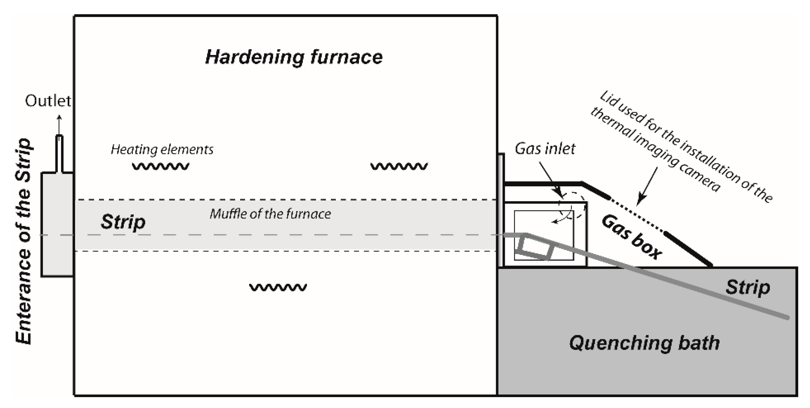
An LBE bath is used as a martempering media in the continuous hardening process which is mainly used to produce thin strips for: Valve steel, springs and blades for the paper & printing industry. Figure 1 illustrates a schematic view of the specific hardening process, before the martensitic transformation step.
The strip is transported within the muffle of the furnace into the LBE bath through a sealing box, a so called gas box. A gas inlet located inside the gas box, which provides the reducing hydrogen atmosphere of the furnace.
Flatness and geometrical defects can still be observed in the thin strips despite all advantages of using LBE as a martempring media in the hardening process. A better comprehension of the process is required in order to investigate how those defects may form.
The uneven temperature difference were referred by many researchers as one of the main reasons for the cause of flatness defects. Thelning [5] discussed the dimensional variation during case hardening and concluded that the thermal stresses, created during cooling, were the main cause for the variations. Moreover, numerical modelling for prediction of the temperature within various steel processes has been widely performed. Some researchers studied the thermomechanical behavior numerically in the solid parts of the casting of steel [6,7,8]. Furthermore, the edge wave of a hot rolled strip after cooling were analyzed by Yoshida [9]. He established a numerical model to predict the temperature and thermal stresses in the strip. He showed that wavy edges can be minimized by having a uniform transverse temperature difference. Wang et al. [10] studied the correlation between the temperature differences, which resulted in thermal stresses and deflection problems of the thermomechanical controlled process (TMCP) plates manufactured by the accelerated cooling process. Various kind of flatness defects, caused by the non-uniform cooling in the different directions, were found. Furthermore, Zhou et al. [11] showed that cooling of a hot rolled strip on the run-out table increases the temperature difference between the center and edges of the strip. This led to an increased buckling tendency. In addition, Wang et al. [12] proved that non-uniform temperature distributions within the strips width are the main reasons for flatness defects, during a run-out table cooling during rolling of hot steel strips. Furthermore, a numerical model was established to predict the amount of thermal stresses originated during cooling period. Here, thermal image measurement data across the transverse direction at the exit of the rolling mill were used as the initial conditions of the strip in the finite element model (FEM) simulations. Wang et al. [13] also developed a numerical model of steel strips during the quenching after the last mill stand in hot strip rolling. This investigation was done in order to predict the flatness of the strip. Also, the results by Wang et al. [14] showed that the wave shape of steel strips during the run-out cooling procedure was mainly caused by uneven transverse temperature and microstructure differences. Moreover, personal communications with experts in the industry [15] has strengthened the influence of the quenching in the molten metal bath on the flatness of the stainless steel strip within the hardening process.
In spite of all the investigations regarding the matter of the temperature on the quality of steel strip, very little focus has been applied on the temperature distribution of the strip beyond the hardening furnace. Therefore, a numerical model was established consisting of the heat transfer of the strip when it leaves the furnace and goes in to the molten metal quenching bath. In addition, for validations of the numerical predictions together with a better understanding of the process, infrared thermal imaging camera measurements were employed. Thus, this study aims to give a better insight into the cooling step of the hardening process as well as to reveal the temperature distribution of the strip during the quenching operation. In addition, this study can be used for a further thermomechanical analysis of the strip. Moreover, the novelty of this work proposes a method to extract surface temperatures of strips in a continuous heat treatment process.
2. Model Description
The numerical model was carried out using Comsol Multiphysics [16]. In this study, the focus was on the temperature distribution of the strip beyond the hardening furnace within the gas box and LBE.
2.1. Mathematical Formulation
In the formulation of the numerical model, the following assumptions were made:
- Within the hydrogen filled gas box, the continuity and energy balance equations combined with the laminar Navier–Stokes equation were solved numerically where thermal interactions between the strip and the hydrogen gas flow take place.
- Within the LBE bath, only heat transfer by conduction was considered as the thermal interaction between the strip and molten metal bath.
- Because of low Reynolds number (around 485, calculated based on inlet geometry) a non-isothermal laminar flow was considered for the gas flow.
- The Mach number was about 0.00093. Thus, a weak compressibility for the flow was also assumed.
- A steady state solution was applied for the numerical model and time dependency effects (transient situation) were neglected.
- The gravitational force was neglected.
Based on these assumptions the following governing equations were solved numerically:
• Continuity equation:
• Momentum equation:
• Energy balance equation:
where is the transpose matrix, is the velocity vector [m/s], is the mass density [kg/m3]. Furthermore, and are the dynamic viscosity of the fluid [Pa·s] and the pressure [Pa], respectively; stands for the identity matrix. In addition, represents the thermal conductivity [W/(m·K)] and defines the heat capacity at a constant pressure [J/kg·K].
2.2. Mesh and the Geometry Used in the Numerical Simulation
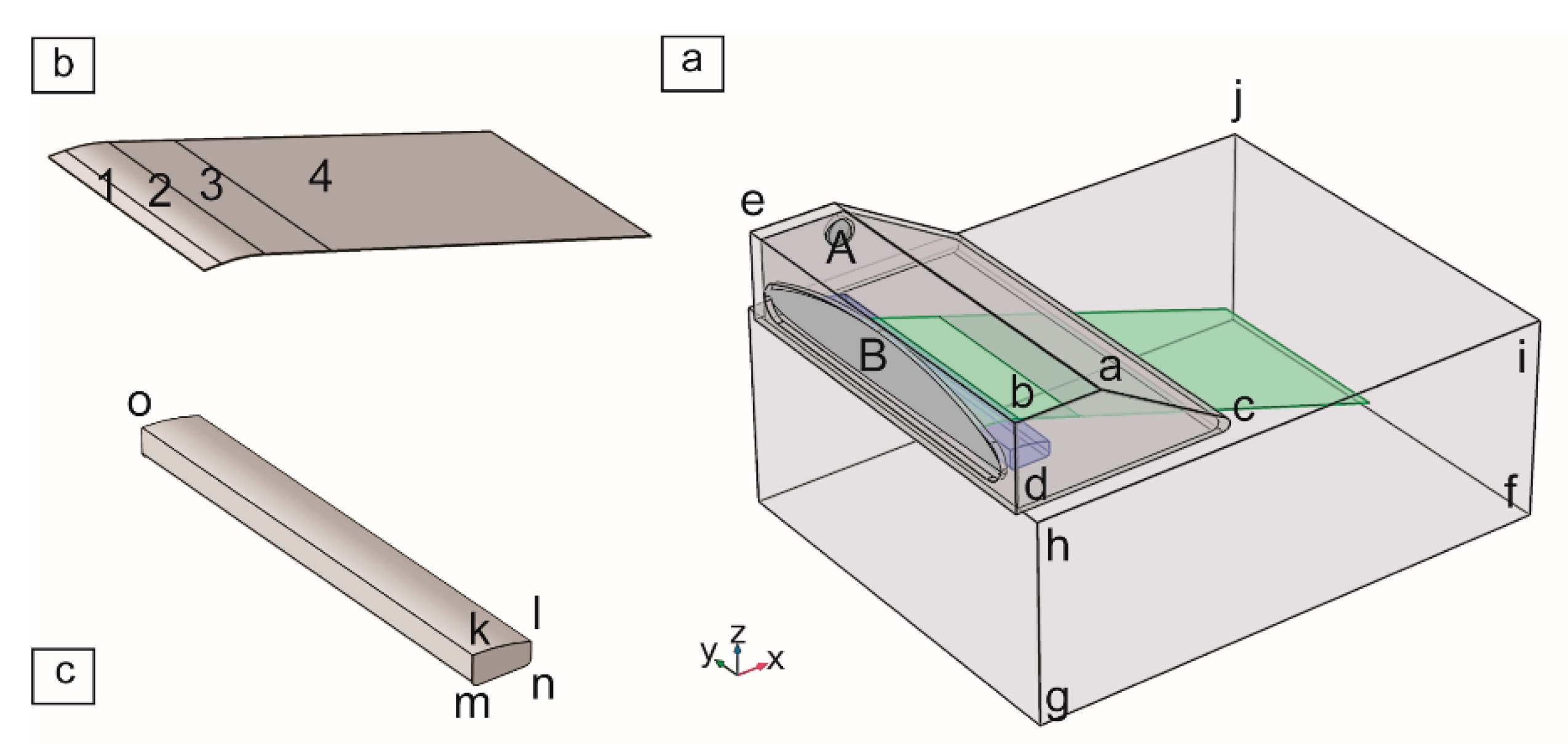
The geometry used in the model was based on the real process conditions at voestalpine in Munkfors, Sweden. A hot stainless steel strip enters the gas box beyond the hardening furnace, which is filled with hydrogen to achieve a reducing atmosphere. Thereafter, the strip is quenched by the Lead-Bismuth eutectic bath. Figure 2 shows a schematic view of the three-dimensional solution domain, for which the governing equations were solved. In addition, a complete list of the dimensions used in the domains is given in Table 1.
Segments 1–4 was used to define the stainless steel strip. This was done to simplify the adjustment of the boundary conditions for each part of the strip. The thickness of the strip was 0.2 mm. Therefore, the strip was assumed as a shell. Surface A implied the gas inlet () while surface B (Area = 31,780 mm2) was set as an outlet.
A model verification was done in order to achieve mesh-independent result together to improve the solution time. 83,197, 278,930 and 545,445 elements were solved numerically. Those grids contains different grid sizes and shapes, due to the complexity of the model. Specifically, in the shape of tetrahedral, pyramid, prism, triangular, edge and vertex elements.
2.3. Method of Solution and Boundary Conditions
Different boundary conditions and initial values were chosen to describe the thermal interaction at the different domains. The boundary conditions contain some process-defined values as well as some assumptions. The labels from Figure 2 are used for a clarification of the given values.
- A moving wall conditions for the Segments 1–3 of the strip (Figure 2b).
- A no-slip condition for the inner side of the ceiling of the gas box.
- Gas inlet (surface A in Figure 2a): . A quantified temperature was considered due to the measured temperature of the walls of the gas inlet.
- Convective heat flux from gas box to air (assumed ): , ,
- Convective heat flux from top surface of the bath to air. Low value of was assumed due to the surface oxidation. , ,
- Pressure outlet for surface B in Figure 2a. and backflow is allowed.
- A typical furnace temperature for the surface B in Figure 2a is .
- A typical set point temperature for the bath is . The placement of this boundary condition was also studied.
2.4. Physical Parameters Used in the Model
The physical parameters of each domains together with dependency of those parameters to the temperature are shown in Table 2.
For the steel strip, the physical parameters of the steel grade AISI 420 or EN 1.4034 were used [18]. Also, the data for LBE bath were extracted from the literature [19]. Trinks et al. [20] introduced a surface emissivity of 0.35 for a bright surface of molten lead. In this research, the same value was assumed as the surface emissivity of the LBE bath. For segments 1 and 2 of the strip in Figure 2b, the values of 0.4 and 0.5 were assumed as their surface emissivity of strip due to the low and high temperatures, respectively. Wen [21], showed that with an increased temperature the value of the surface emissivity increased as well for AISI 420. In addition, the high value of surface emissivity was assumed for the strip due to the bright surface of the strip at the exit of the furnace filled with reducing atmosphere. Wen [21] also described that the emissivity alters between 0.4 to 0.7, due to the steel grade and temperature. Therefore, an emissivity value of 0.6 was assumed for the outlet or interface of the furnace and the gas box. This was done to consider the radiated heat from the furnace, i.e., the steel muffle located inside of the furnace. In addition, a value of 0.4 was assumed for the inner side of the gas box which has a lower temperature. Furthermore, a regression of the data, taken from NIST (National Institute of Standard and Technology) was used for physical properties of the hydrogen gas. The NIST data was extracted from the literature [22,23,24]. A regression of the data was also considered for the thermal conductivity of strip and gliding material. A typical high temperature board used in this application was assumed for a gliding material. Also, the gas box’s wall was estimated to be equivalent to an AISI 4340 alloy.
3. Process Temperature Measurements
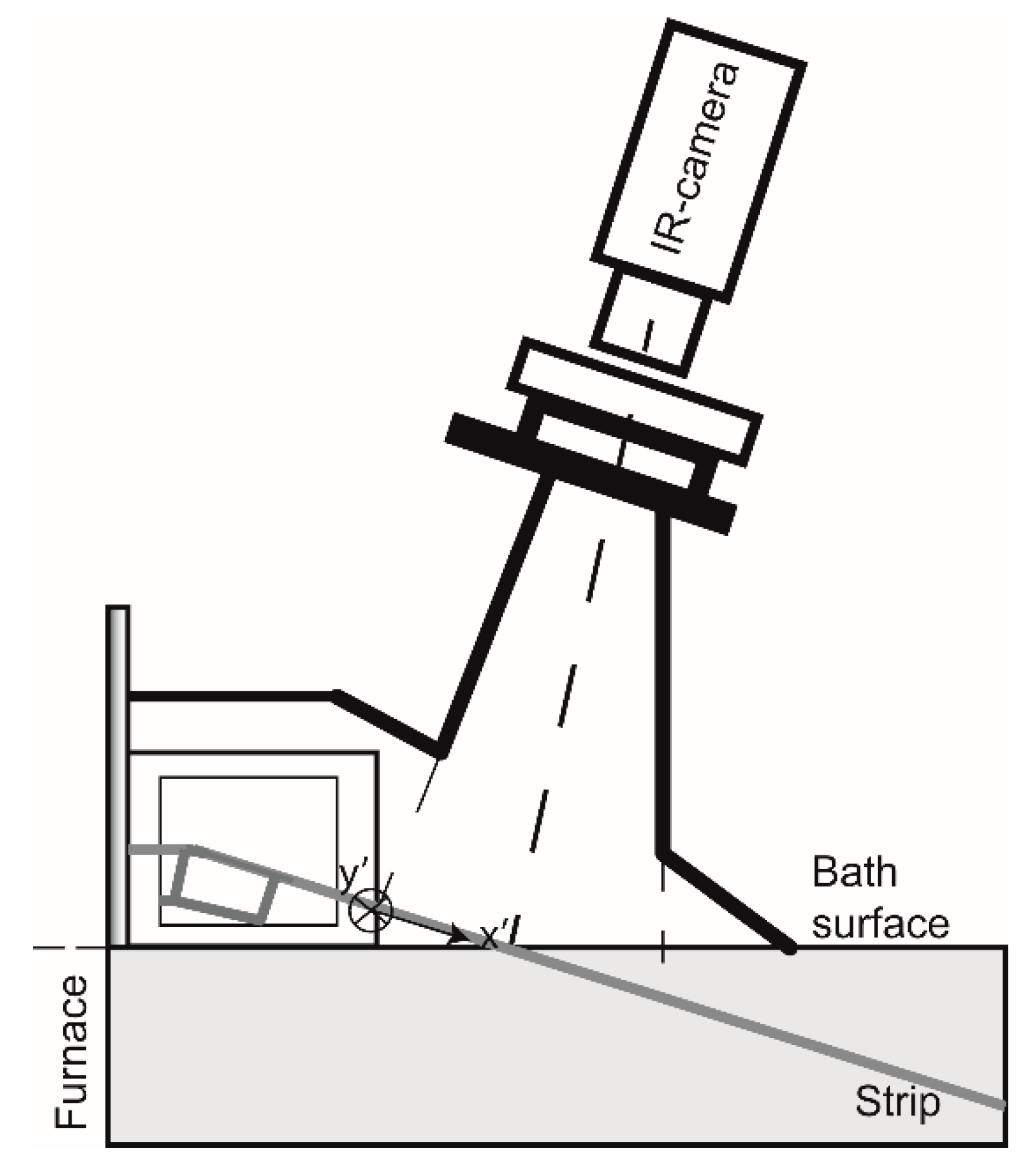
The temperature of the strip was measured by using a PYROVIEW 320 thermal imaging camera (DIAS Infrared GmbH, Dresden, Germany), during steady state condition of the process to gain consistent results. This was done in order to establish a proper boundary condition for the finite element model as well as to investigate the accuracy of the numerical model. The measured range was between 300 to 1200 °C including 320 × 256 pixels. Also, the segment of the strip located just before it entered the bath was targeted for the measurements. The limits for installation the camera such as its working temperature and limited accessibility at the gas box caused the choice of this area for measurements. A surface emissivity of 0.4 was set for the camera which is the same as was used in the numerical model. Furthermore, a ±2% of measured temperature was given as the measurement uncertainty by the manufacturer [25]. This uncertainty is shown as an error bar in the results. Figure 3 shows the schematic view of the temporary measurement setup.
4. Results and Discussion
4.1. Model Verification
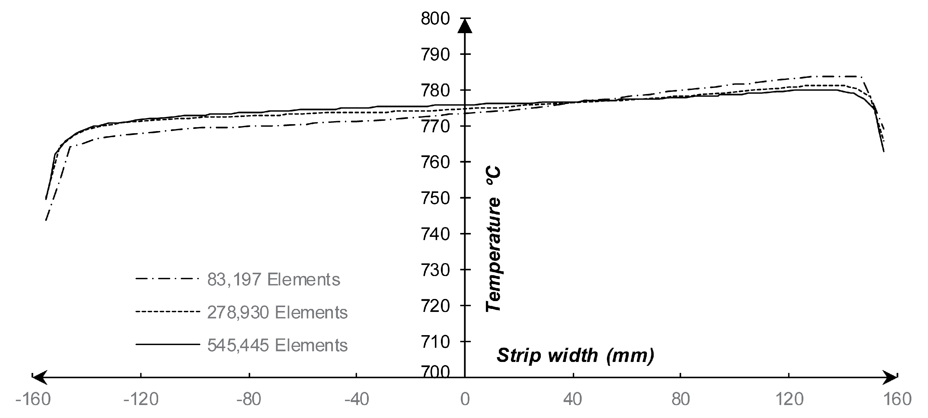
The computational domains were solved for three numbers of mesh elements. This was done in order to study if an improved convergence time together with mesh-independent results could be obtained. Solutions times with a Win7 PC with a 3.40 GHz Intel Core i7 CPU and a 32 GB RAM were: Mesh-1 83197 = 26 min, 19 s; mesh-2 278930 = 2 h, 41 min; mesh-3 545445 = 6 h, 5 min. The temperature distribution across a line (strip’s width) was used for the verification. This line was located 63 mm before the interface of the strip and the bath. The results are shown in Figure 4.
The results show that the model, meshed with 83,197 shows a maximum 0.4% temperature deviation in comparison with the model meshed with 545,445 elements. Furthermore, the deviation between a model with 278,930 mesh elements and a model with 545,445 elements was 0.1% meanwhile the solution time was about 50% less. Therefore, the numerical model containing 278,930 elements was considered for the further investigations.
4.2. Model Validation
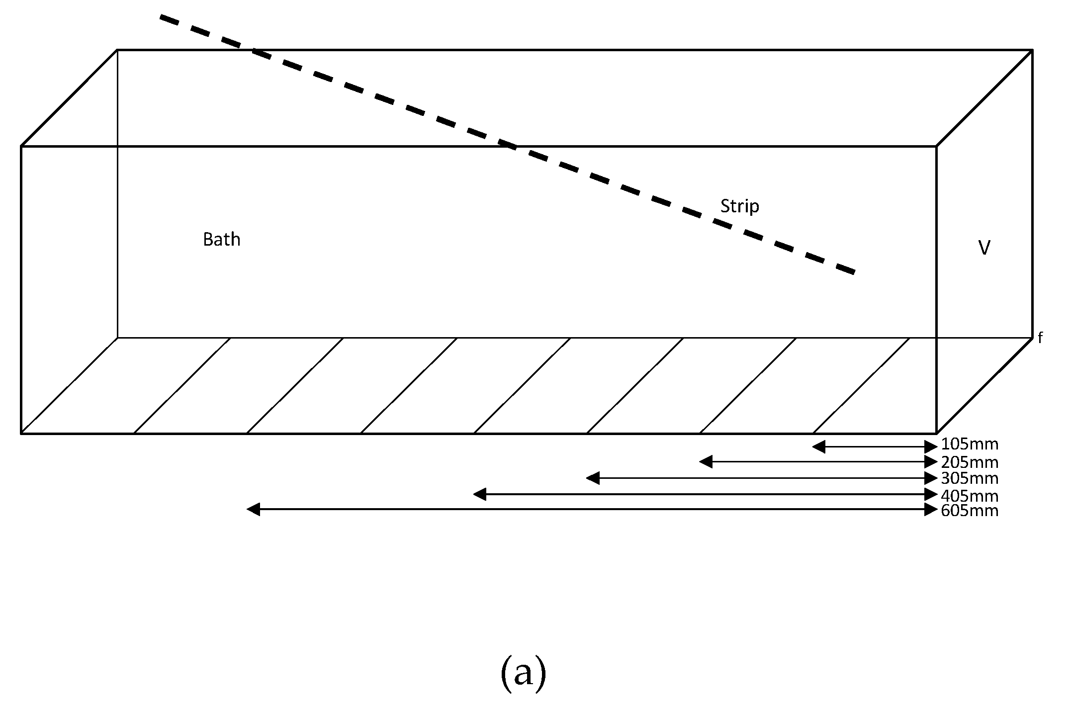
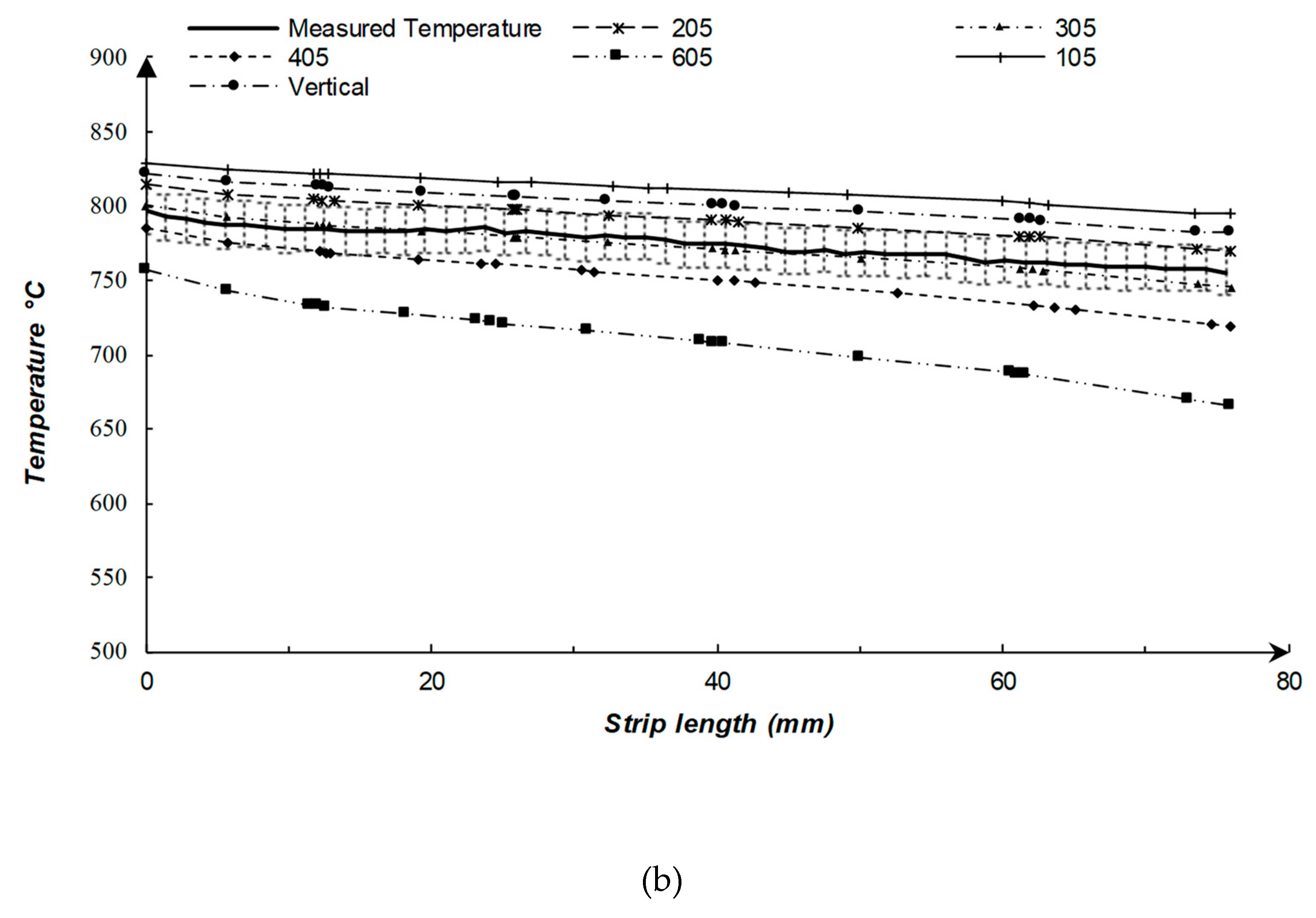
The computational domains were solved numerically in order to explain the quenching of the thin stainless steel strip beyond the hardening furnace. For solving such a complicated numerical model some assumptions needed to be considered. A constant temperature was defined as the boundary condition of the bath. Meanwhile the size and the placement of this boundary condition needed to be assumed. Therefore, the numerical model were solved for different boundary conditions of the size and placement, which is illustrated schematically in Figure 5a. Furthermore, the results were compared with measured temperatures from the real process (Figure 5b). The comparison was done within the gas box along the center of the strip in longitudinal direction ended 21 mm away from the bath interface with the length of 80 mm.
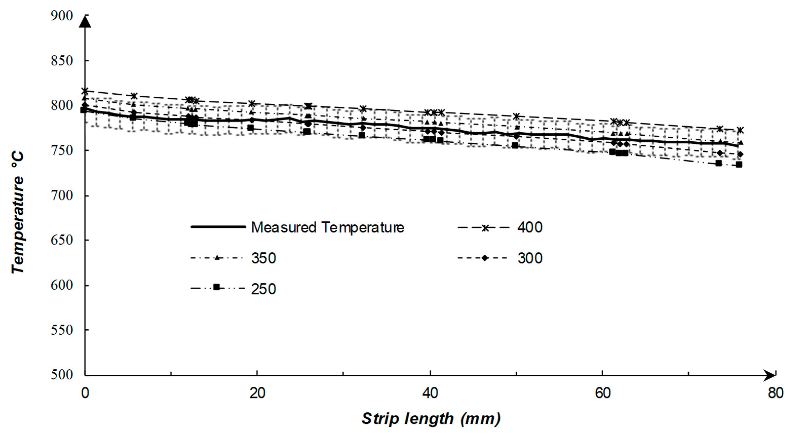
It can be seen that a proper agreement can be observed by assuming 305 mm distance as the boundary condition of the bath. The temperature of the center of the strip decreased from 797 to 755 °C (i.e., 42 °C) and 799 to 746 °C (i.e., 53 °C) according to the temperature measurement and the numerical model prediction, respectively. It can be also seen that the temperature of strip decreases dramatically within the gas box. By considering 305 mm distance as the boundary condition of the bath, the assumed temperature for the bath is also validated. The results are presented by Figure 6. The temperature is seen to be decrease with a decreased bath temperature and an increased strip length. A typical bath temperature for this process is 300 °C and the results of the predicted model by assuming 300 °C in the model shows a proper accordance to the real process temperature measurements.
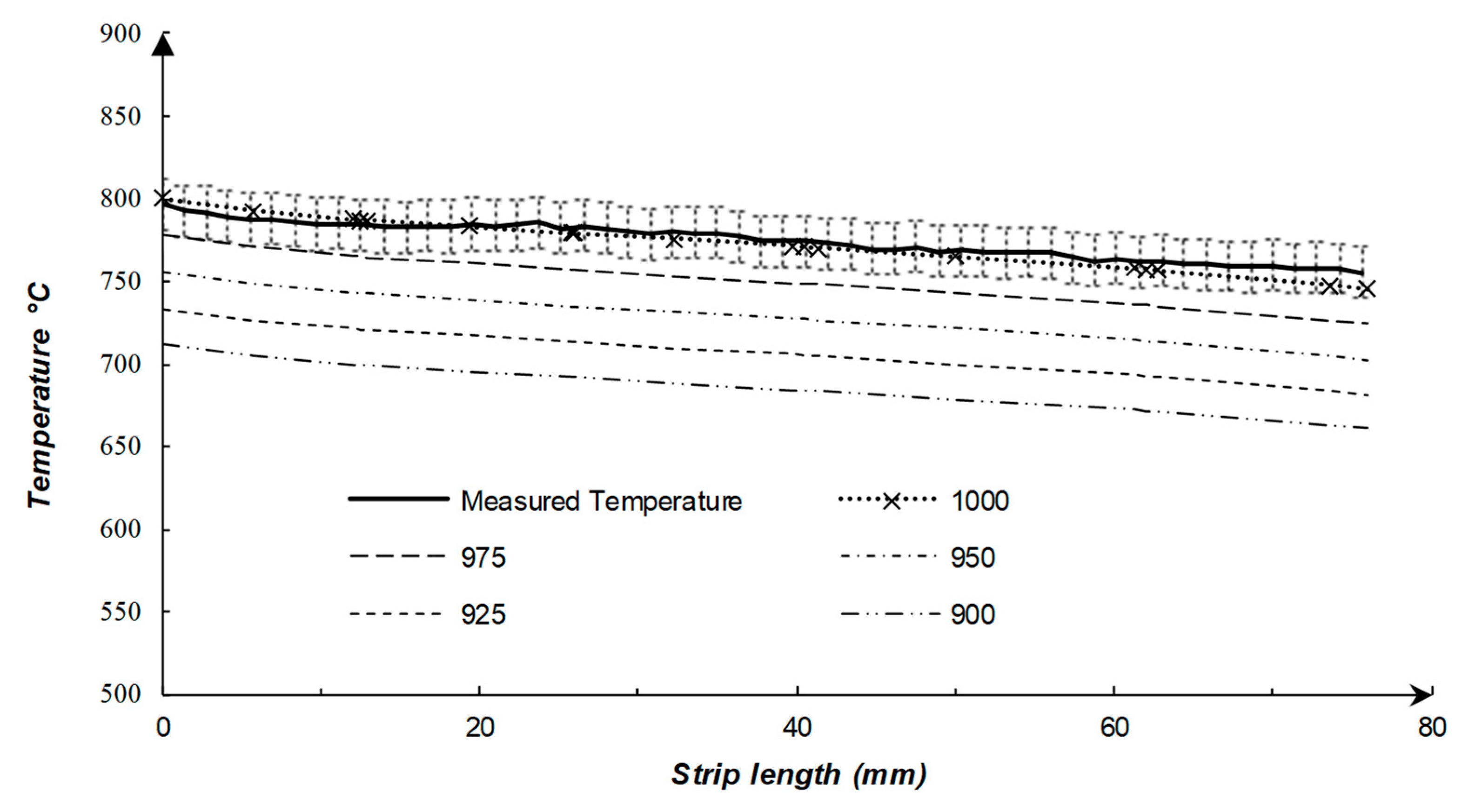
Furthermore, a constant value of the furnace temperature was considered in the model. A typical furnace temperature is 1000 °C. Meanwhile the temperature might be altered at surface B in Figure 2a which represents the furnace temperature. Therefore, the accordance of this assumption on the system was studied numerically and compared to the real process data. The results are shown in Figure 7. It can be seen, that considering a constant temperature value for the furnace, i.e., 1000 °C, is a fairly good assumption. The temperature is seen to increase with an increased furnace temperature.
4.3. The Numerical Model and the Measured Temperature
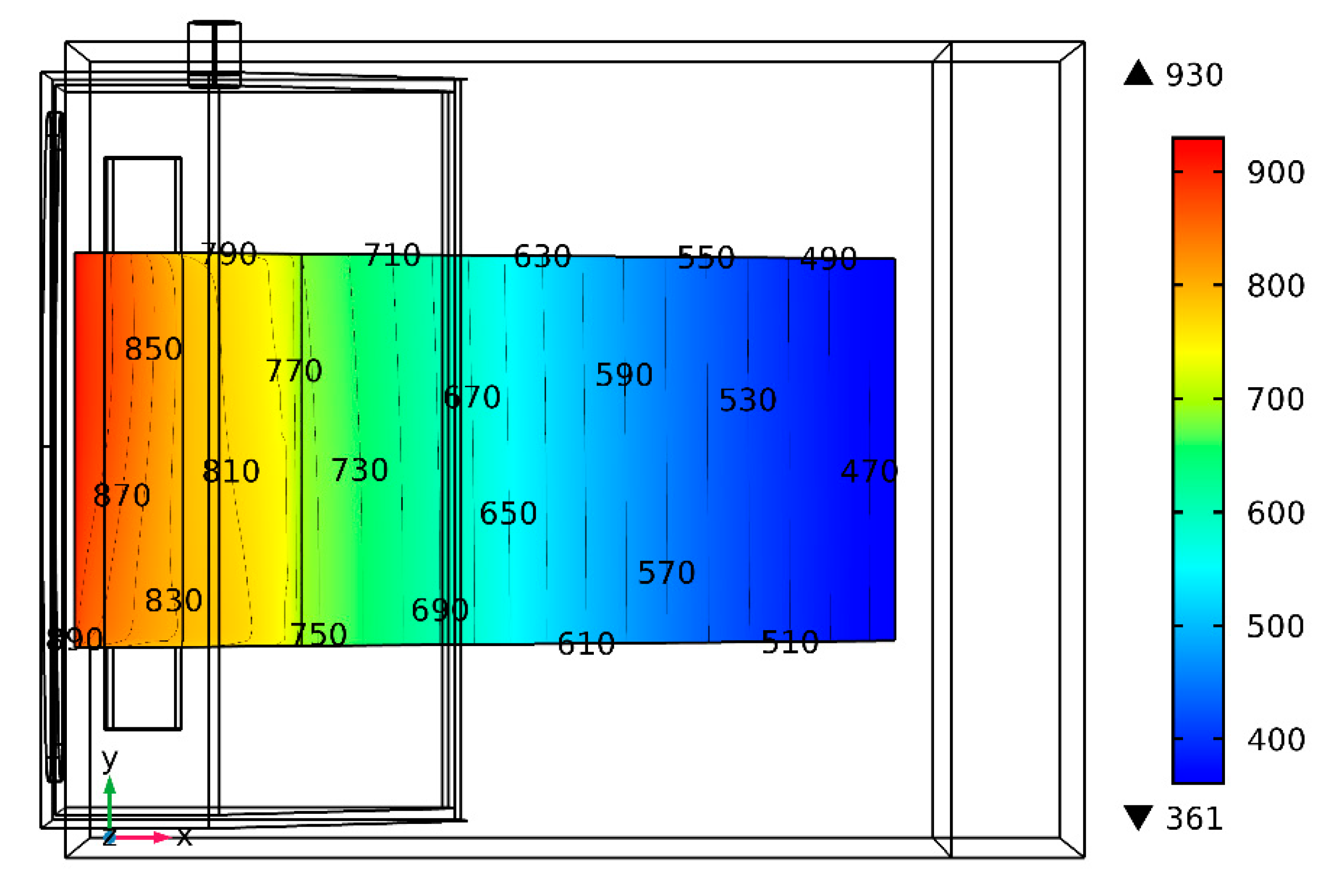
The temperature distribution of the hydrogen gas within the gas box at the surface just above the strip is illustrated in Figure 8.
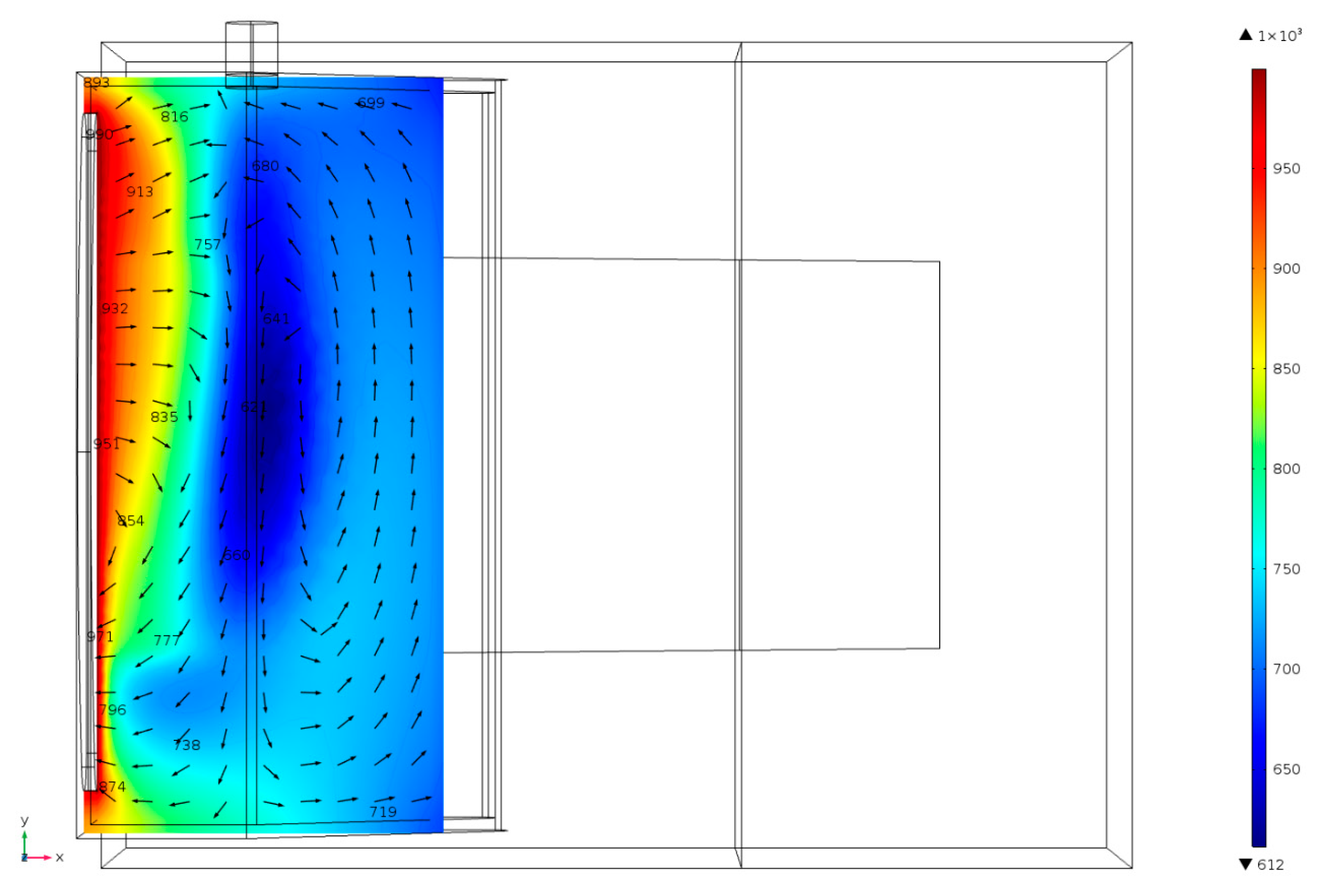
It can be seen that the temperature of the hydrogen flow decreases dramatically in the gas box, which lead to an uneven cooling effect in the stainless steel strip. The coldest area was located around the gas inlet and it has a temperature of 200 °C. Furthermore, the result shows that a cold flow of hydrogen gas propagates to the other side of gas box, far from the gas inlet. The temperature of the flow at the area between the gas inlet and the furnace surface was around 816 °C. Meanwhile, this value was about 734 °C at the other side of gas box in the y-direction. Figure 9 shows the predicted temperature of the strip cooled by the hydrogen flow and the quenching bath.
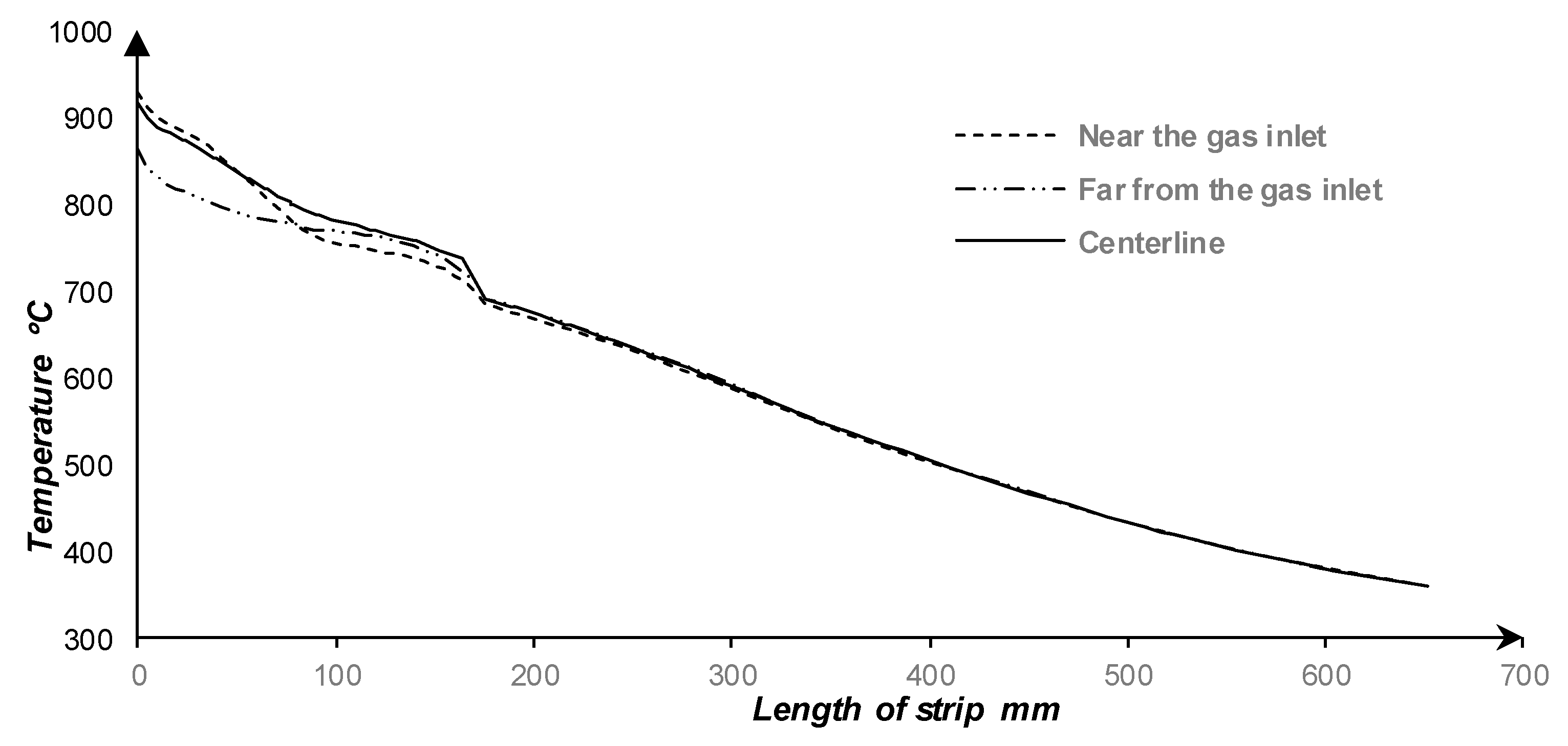
It can be seen, that the temperature of the strip decreased from 1000 °C to around 750 °C within the gas box. Thereafter, during quenching the temperature decreased to 470 °C in the LBE bath. However, the gas flow was preliminary designed to provide a reducing atmosphere in the furnace. Also, significant non-uniform temperature patterns were visible, especially across the strips’ transverse direction (y-direction) in the gas box. The predicted temperature along the two edges and the center of the strip are shown in Figure 10. The temperature decreased from around 1000 °C to 350 °C at a 650 mm strip length. The strip cooled non-uniformly before a length of 175 mm where quenching by molten metal occurred.
At the position about 100 mm, where the gas inlet locates, notable temperature differences between the center of strip and the edge near the gas inlet can be observed. This transverse temperature difference can be up to 24 °C. Meanwhile, at the area between 0–100 mm a significant transverse temperature difference can be observed between the far and near edges from the gas inlet. Specifically, it can be up to 69 °C at the length of 24 mm. The result indicates the concentration of cold hydrogen flow at the area far from the gas inlet between the length of 0–100 mm of strip, which can be observed in Figure 8, and Figure 9. During quenching in a molten metal bath, gradually a uniform temperature pattern across the width of strip becomes visible.
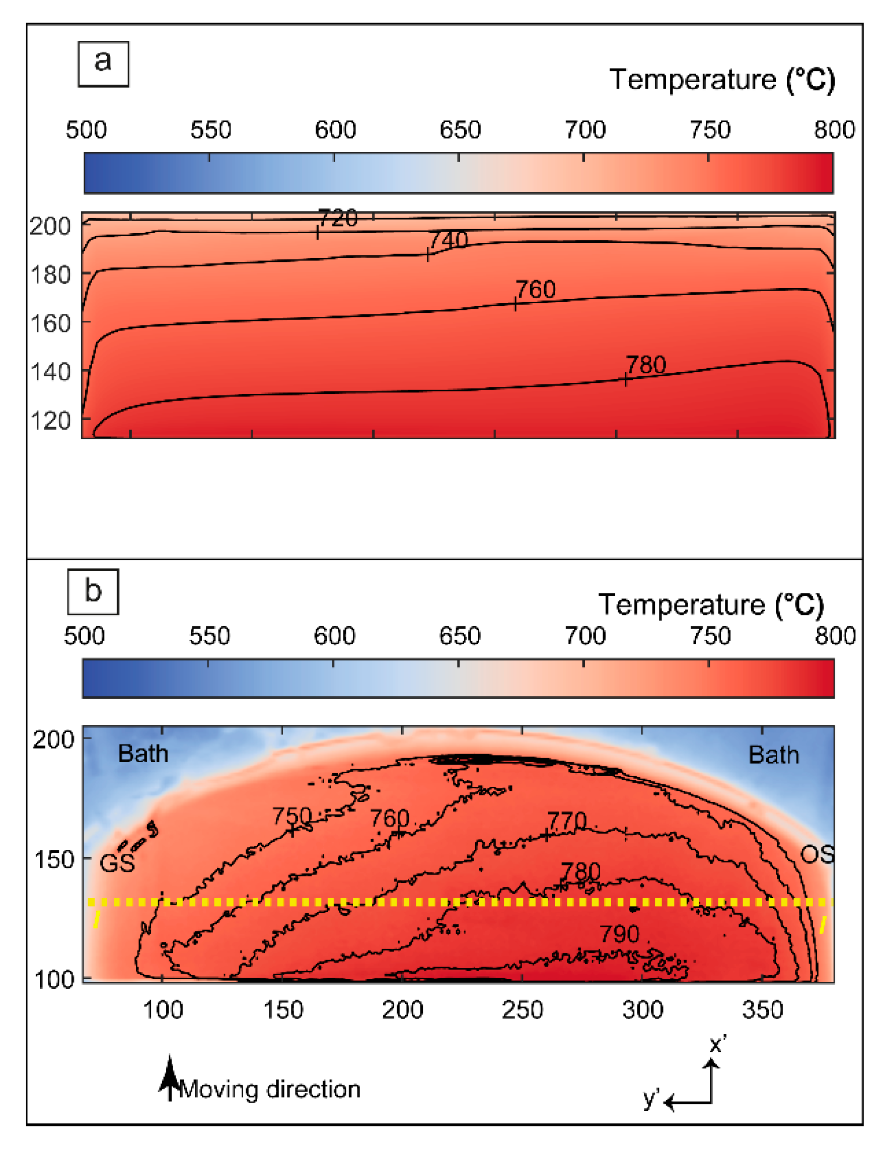
In this study, an infrared thermal imaging camera was employed in order to compare the predicted results to the real process temperature to obtain a better understanding of the process. Figure 11 compares the results of the numerical model with the measured data at the area covered by the thermal imaging camera.
The temperature results from thermal imaging camera are shown in Figure 11b. Meanwhile the predicted results of the numerical model for the measured temperature are shown in Figure 11a. The gas inlet side is shown as GS in Figure 11 and the operator side is defined by OS. The strip found to be slightly buckled within the gas box during the real process temperature measurements. This can be seen as the curved shape of the strip in Figure 11. Both the predicted and measured results at this section of strip indicate that the temperature drops near to the gas inlet. Moreover, the temperature of the strip decreases about 250 °C within the gas box from the furnace temperature, which is typically around 1000 °C. The line I-I is used for comparison of the predicted results and the measured value and the result is shown in Figure 12. The position of this line is about 63 mm from the bath interface. However, defining the same line for the numerical model and the thermal imaging analysis is not an easy task.
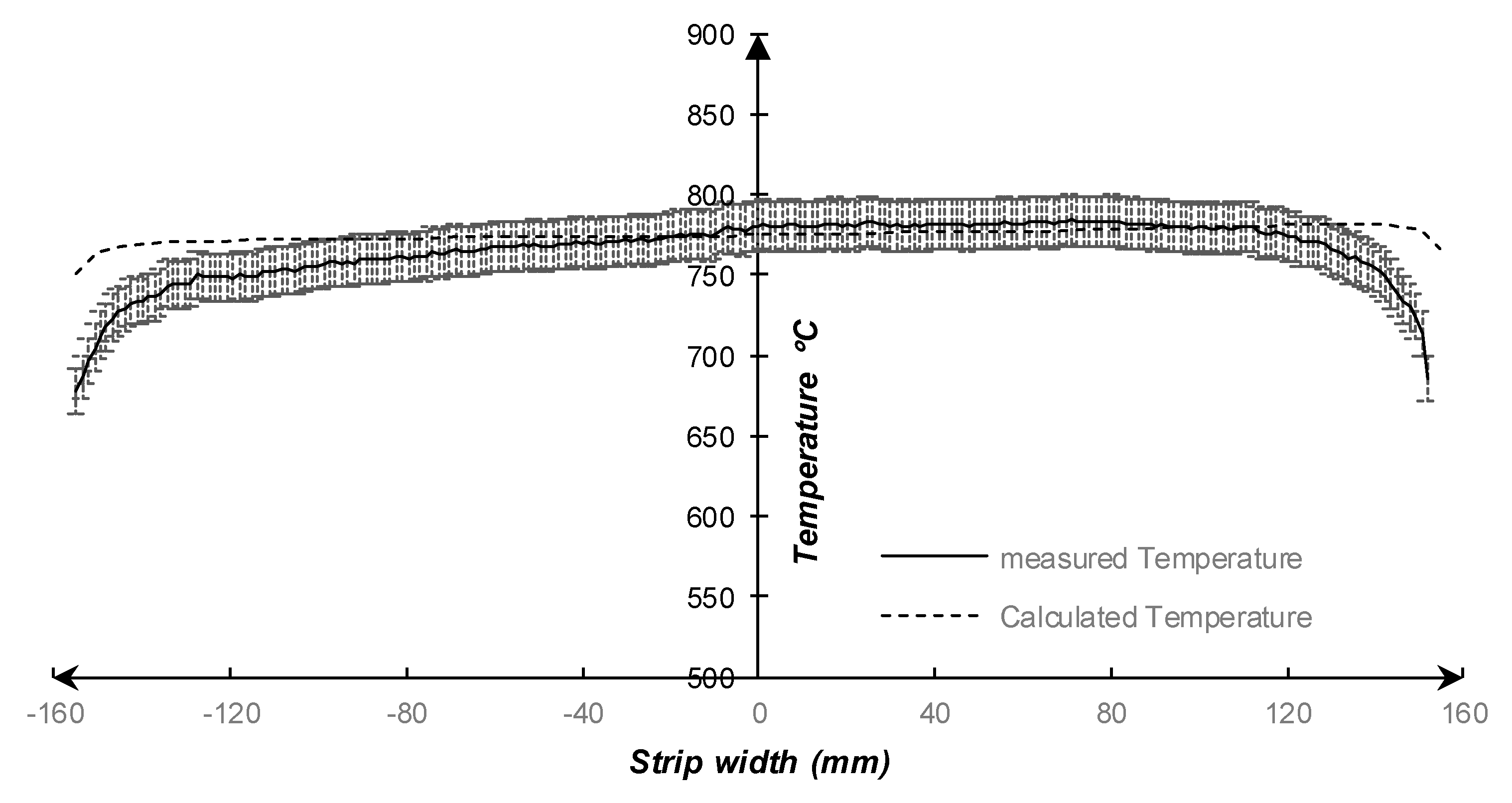
As it can be seen in Figure 12, the same tendency can be observed from both the predicted and measured temperatures. Specifically, a proper agreement can be observed explicitly at the center of the strip where the deviation of calculated result to the measured value was about 0.6%. The maximum measured temperature was 784 °C while this value was about 782 °C for the numerical model. However, there was about a 50 mm difference between their locations. The difference between the minimum temperature for the calculated value and the measured value was about 9% at the edge of the strip, which can arise from the limitations of both the numerical model predictions and infrared temperature measurements. The results of the thermal imaging camera can be affected by different parameters. Minkina and Dudzik [26] classified the errors in temperature measurement performed by IR cameras into:
- Errors of measuring method;
- Errors of calibration;
- Errors of electric path.
Errors of measuring method contain: An effect of the ambient radiation detected directly by the camera or reflected by the surface, an ambient temperature, and an incorrect setting for the surface emissivity of the object. The surface emissivity of the object greatly depends on the temperature and the state of the surface together with the direction of observation [26]. Also, Wen [21] showed that the surface emissivity of strip changes by the temperature. During the real process temperature measurement, this effect had been observed. The results of measurement can vary up to 4% from emissivity of 0.3 and 0.4. Therefore, defining a reliable constant value of the emissivity for the camera to measure the whole object area isn’t an easy task. In addition, the strip has been found to be buckled in the gas box. Therefore, this can lead to the changes in the state of the surface. The height of the IR-camera is an essential parameter to obtain accurate results due to the configurations of the lens. It should be set based on the Horizontal Field of View (HFOV) and Vertical Field of View (VFOV). Therefore, HFOV and VFOV changed during the measurement for the top and edges due to existence of a buckled strip. Consequently, reflections and errors in temperature measurements can be caused by this incident. Therefore, the uncertainty of the temperature measurements can be more than 4%, which was the uncertainty of the measurements caused by changes in the surface emissivity. Notably, ±2% of the measured value is mentioned as the calibration error of the camera [25]. This value of uncertainty is considered when the camera is operated under specified laboratory conditions for an ambient temperature of 25 °C and a black body radiator [25]. Therefore, the uncertainty might be significantly higher in real process temperature measurements. The errors of the electric path of the camera are below ±1% for 25 °C as the ambient temperature. In general, errors of measuring method are the main causes of the uncertainty and can reach up to several percent [26]. The limitations of the numerical model are not negligible. Many boundary conditions based on the real process were employed in the current complex heat transfer model. Also, many physical properties of each domain vary with the temperature. These parameters where chosen to be as accurate as possible. However, defining a precise value and a temperature correlation for all physical properties is still a great struggle. Furthermore, it is possible that localized turbulence occurs at the very edges of the strip and may consequently cause a higher cooling.
Overall, the difference between the predicted results and measured data in Figure 12 can be explained by those errors, specifically at the edges. By neglecting the data 20 mm from each edge, the maximum temperatures for the calculated and measured data are 782 °C and 784 °C, respectively. Meanwhile, the minimums are 770 °C and 743 °C. The temperature difference between the maximum and minimum in the y-direction (transverse direction), at the I-I line defined in Figure 11 is 12 °C and 41 °C for predicted data and measured value, respectively.
5. Conclusions
In this study, an investigation of the temperature distribution within the molten metal quenching step of a continuous hardening process was carried out based on both numerical modelling and infrared thermal imaging measurements. The conclusions of this study may be summarized as follows:
- The methodology of creating a numerical model of a restricted part of a continuous hardening process with experimental validation generates the surface temperature distribution along the thin strip. This allows isolated studies of parts of the process to be analyzed.
- An infrared thermal imaging camera can effectively be used for validation and for improving the boundary conditions of the numerical model. In addition, the measurements reveal the surface of the strip to be buckled, which could not be identified by the numerical model.
- Gas designed to provide a reducing atmosphere in the hardening furnace can have a significant cooling effect. Therefore, a more symmetrical design helps to decrease transverse temperature gradient and possibly improve the flatness.
- Less agreement between the numerical model and the process temperature measurements were observed at the edges. The discrepancy is likely caused by the curvature of the strip, which increases the measurement uncertainty, especially at the edges. However, localized turbulence may occur at the edges of the strip, which may consequently cause a higher localized cooling. Therefore, if higher precision at the edges are necessary localized, turbulence should be considered with low Reynolds turbulence models.
Author Contributions
Conceptualization, N.Å.I.A. and A.T.; methodology, P.P., N.Å.I.A. and A.T.; validation, P.P., N.Å.I.A. and A.T.; formal analysis, P.P., N.Å.I.A. and A.T.; investigation, P.P.; resources, A.T., P.G.J.; data curation, P.P.; writing—original draft preparation, P.P.; writing—review and editing, P.P., N.Å.I.A., A.T. and P.G.J.; visualization, P.P. and N.Å.I.A.; supervision, N.Å.I.A. and A.T.; project administration, A.T.; funding acquisition, A.T.
Funding
This research received no external funding.
Acknowledgments
The authors would like to thank Chris Millward and Stellan Ericsson of voestalpine Precision Strip AB, for fruitful discussions and a great support with the temperature measurements as well as Nihat Palanci of Snesotest, Sweden for providing the possibility to use the infrared camera for the industrial measurements. In addition the authors appreciate the valuable discussions with Dong-Yuan Sheng regarding mathematical modelling. This study was carried out with a financial support from the Regional Development Council of Dalarna, Regional Development Council of Gävleborg, County Administrative Board of Gävleborg, the Swedish Steel Producers′ Association, Dalarna University, Sandviken Municipality and voestalpine Precision Strip AB.
Conflicts of Interest
The authors declare no conflict of interest.
References
- Webster, H.; Laird, W.J. Martempering of Steel, Heat Treating. In ASM Handbook; ASM International: Materials Park, OH, USA, 1991; Volume 4, pp. 137–151. [Google Scholar]
- Ebner, J. Bright Heat Treating of Carbon Steel Strip Using a Lead Quench. Mach. Steel Austria 1983, 4, 83–90. [Google Scholar]
- Lochner, H. Hardening of strip in a molten-metal bath or hydrogen jet cooler. Steel Times 1994, 222, 350. [Google Scholar]
- Lochner, H. Steel strip hardening and tempering lines for medium and high carbon steels and alloyed grades part I: Production lines with liquid metal quenching. In Proceedings of the IFHTSE—International Federation for Heat Treatment and Surface Engineering, Vienna, Österreich, 25–29 September 2006; p. 43. [Google Scholar]
- Thelning, K.-E. 7—Dimensional changes during hardening and tempering. In Steel and its Heat Treatment, 2nd ed.; Butterworth-Heinemann: Oxford, UK, 1984; p. 581. [Google Scholar] [CrossRef]
- Rappaz, M. Modelling of microstructure formation in solidification processes. Int. Mater. Rev. 1989, 34, 93–124. [Google Scholar] [CrossRef]
- Choudhary, S.K.; Mazumdar, D.; Ghosh, A. Mathematical Modelling of Heat Transfer Phenomena in Continuous Casting of Steel. ISIJ Int. 1993, 33, 764–774. [Google Scholar] [CrossRef]
- Koric, S.; Hibbeler, L.C.; Liu, R.; Thomas, B.G. Multiphysics Model of Metal Solidification on the Continuum Level. Numer. Heat Transf. Part B Fundam. 2010, 58, 371–392. [Google Scholar] [CrossRef]
- Yoshida, H. Analysis of Flatness of Hot Rolled Steel Strip after Cooling. Trans. Iron Steel Inst. Jpn. 1984, 24, 212–220. [Google Scholar] [CrossRef]
- Wang, S.-C.; Chiu, F.-J.; Ho, T.-Y. Characteristics and prevention of thermomechanical controlled process plate deflection resulting from uneven cooling. Mater. Sci. Technol. 1996, 12, 64–71. [Google Scholar] [CrossRef]
- Zhou, Z.; Lam, Y.; Thomson, P.F.; Yuen, D.D.W. Numerical Analysis of the Flatness of Thin, Rolled Steel Strip on the Runout Table. Proc. Inst. Mech. Eng. B J. Eng. Manuf. 2007, 221, 241–254. [Google Scholar] [CrossRef]
- Wang, X.; Yang, Q.; He, A. Calculation of thermal stress affecting strip flatness change during run-out table cooling in hot steel strip rolling. J. Mater. Proc. Technol. 2008, 207, 130–146. [Google Scholar] [CrossRef]
- Wang, X.-D.; Li, F.; Jiang, Z.-Y. Thermal, Microstructural and Mechanical Coupling Analysis Model for Flatness Change Prediction During Run-Out Table Cooling in Hot Strip Rolling. J. Iron Steel Res. Int. 2012, 19, 43–51. [Google Scholar] [CrossRef] [Green Version]
- Wang, X.; Li, F.; Yang, Q.; He, A. FEM analysis for residual stress prediction in hot rolled steel strip during the run-out table cooling. App. Math. Model. 2013, 37, 586–609. [Google Scholar] [CrossRef]
- Eriksson, S.; R&D Process Technology, Voestalpine Precision Strip AB, Munkfors, Sweden. Personal communication, 2012.
- COMSOL. COMSOL Multiphysics v.5.1. Available online: https://www.comsol.se/release/5.1 (accessed on 3 May 2019).
- COMSOL Multiphysics. Heat Transfer Module User’s Guide; Version 5.1; COMSOL AB: Stockholm, Sweden, 2015. [Google Scholar]
- Spittel, M.; Spittel, T. Steel symbol/number: X46Cr13/1.4034. In Metal Forming Data of Ferrous Alloys—Deformation Behaviour; Warlimont, H., Ed.; Springer: Berlin/Heidelberg, Germany, 2009; p. 588. [Google Scholar] [CrossRef]
- Nuclear Science Committee. Handbook on Lead-Bismuth Eutectic Alloy and Lead Properties, Materials Compatibility, Thermal-Hydraulics and Technologies; OECD Nuclear Energy Agency: Paris, France, 2007.
- Trinks, W.; Mawhinney, M.H.; Shannon, R.A.; Reed, R.J.; Garvey, J.R. Saving Energy in Industrial Furnace Systems. In Industrial Furnaces; John Wiley & Sons, Inc.: Hoboken, NJ, USA, 2007; p. 190. [Google Scholar] [CrossRef]
- Wen, C.-D. Investigation of steel emissivity behaviors: Examination of Multispectral Radiation Thermometry (MRT) emissivity models. Int. J. Heat Mass Transf. 2010, 53, 2035–2043. [Google Scholar] [CrossRef]
- Kunz, O.; Klimeck, R.; Wagner, W.; Jaeschke, M. The GERG-2004 Wide-Range Equation of State for Natural Gases and Other Mixtures; GERG Technical Monograph 15 and Fortschr.-Ber., VDI-Verlag: Düsseldorf, Germany, 2007; p. 1. [Google Scholar]
- Leachman, J.W.; Jacobsen, R.T.; Penoncello, S.G.; Lemmon, E.W. Fundamental Equations of State for Parahydrogen, Normal Hydrogen, and Orthohydrogen. J. Phys. Chem. Ref. Data 2009, 38, 721–748. [Google Scholar] [CrossRef]
- McCarty, R.D.; Hord, J.; Roder, H. Selected Properties of Hydrogen (Engineering Design Data); National Engineering Lab. (NBS): Boulder, CO, USA, 1981; p. 1. [Google Scholar]
- DIAS Infrared Systems. Available online: http://www.webcitation.org/785ncpRm6 (accessed on 3 May 2019).
- Minkina, W.; Dudzik, S. Errors of Measurements in Infrared Thermography. In Infrared Thermography; John Wiley & Sons, Ltd.: Hoboken, NJ, USA, 2009; p. 61. [Google Scholar] [CrossRef]
Figure 1.
Schematic view of the hardening process before a martensitic phase transformation at voestalpine, Presicion Strips AB, Munkfors, Sweden.
Figure 1.
Schematic view of the hardening process before a martensitic phase transformation at voestalpine, Presicion Strips AB, Munkfors, Sweden.

Figure 2.
Computational domains, dimensions are found in Table 1: (a) Three-dimensional solution domains, (b) stainless steel strip, (c) gliding material.
Figure 2.
Computational domains, dimensions are found in Table 1: (a) Three-dimensional solution domains, (b) stainless steel strip, (c) gliding material.

Figure 3.
Schematic view of the temporary measurement setup used in the industrial hardening process.
Figure 3.
Schematic view of the temporary measurement setup used in the industrial hardening process.

Figure 4.
The results of the model verification by temperature predictions across the width of strip.
Figure 4.
The results of the model verification by temperature predictions across the width of strip.

Figure 5.
Validation of assumed boundary condition for the bath size and the placement. (a) Schematic view of the bath with different size and placement of boundary condition; (b) temperature results.
Figure 5.
Validation of assumed boundary condition for the bath size and the placement. (a) Schematic view of the bath with different size and placement of boundary condition; (b) temperature results.


Figure 6.
Validation of assumed boundary condition for the bath temperature.

Figure 7.
Validation of assumed boundary condition for the furnace temperature.

Figure 8.
Hydrogen flow temperature (°C).

Figure 9.
Temperature pattern within the strip (°C).

Figure 10.
Predicted temperature trajectories along the two edges and at the center of the strip.

Figure 11.
Temperature results: (a) Predicted temperature from the model, (b) temperature measured by thermal imaging camera.
Figure 11.
Temperature results: (a) Predicted temperature from the model, (b) temperature measured by thermal imaging camera.

Figure 12.
Comparison of the measured temperature with predicted value across the line I-I defined in Figure 11.
Figure 12.
Comparison of the measured temperature with predicted value across the line I-I defined in Figure 11.


Table 1.
Dimensions of computational domains (mm). The distances are defined in Figure 2.
Table 1.
Dimensions of computational domains (mm). The distances are defined in Figure 2.
| Strip (Figure 2b) | 1 | 2 | 3 | 4 | |||
| 310.0 × 23.5 × 0.2 | 310.0 × 61.3 × 0.2 | 310.0 × 97.0 × 0.2 | 310.0 × 500.0 × 0.2 | ||||
| LBE Bath (Figure 2a) | |||||||
| 805.0 | 300.0 | 645.0 | |||||
| Gas Box1 (Figure 2a) | 2 | ||||||
| 129.8 | 222.6 | 317.6 | 10 | 130.0 | 585.0 | ||
| Gliding Material (Figure 2c) | 2 | 2, | |||||
| 15.8 | 49.0 | 25.0 | 59.9 | 195 | 5 | 450.0 | |
1 The thickness is 10 mm. 2 R: Radius.
Table 2.
Physical properties of each domains.
| Property | Value (s) | Unit | ||
|---|---|---|---|---|
| Strip | k | Thermal conductivity | ||
| ε | Surface emissivity | - | ||
| Wall of the Gas Box | k | Thermal conductivity | ||
| ρ | Density | |||
| Heat capacity | ||||
| ε | Surface emissivity | - | ||
| Hydrogen | k | Thermal conductivity | ||
| ρ | Density | |||
| Heat capacity | ||||
| µ | Dynamic viscosity | |||
| γ | Ratio of specific heat | - | ||
| LBE | k | Thermal conductivity | ||
| ρ | Density | |||
| Heat capacity | ||||
| ε | Surface emissivity | - | ||
| Gliding Material | k | Thermal conductivity | ||
| ρ | Density | |||
| Heat capacity | ||||
© 2019 by the authors. Licensee MDPI, Basel, Switzerland. This article is an open access article distributed under the terms and conditions of the Creative Commons Attribution (CC BY) license (http://creativecommons.org/licenses/by/4.0/).
Share and Cite
MDPI and ACS Style
Pirouznia, P.; Andersson, N.Å.I.; Tilliander, A.; Jönsson, P.G. An investigation of the Temperature Distribution of a Thin Steel Strip during the Quenching Step of a Hardening Process. Metals 2019, 9, 675. https://doi.org/10.3390/met9060675
AMA Style
Pirouznia P, Andersson NÅI, Tilliander A, Jönsson PG. An investigation of the Temperature Distribution of a Thin Steel Strip during the Quenching Step of a Hardening Process. Metals. 2019; 9(6):675. https://doi.org/10.3390/met9060675
Chicago/Turabian StylePirouznia, Pouyan, Nils Å. I. Andersson, Anders Tilliander, and Pär G. Jönsson. 2019. "An investigation of the Temperature Distribution of a Thin Steel Strip during the Quenching Step of a Hardening Process" Metals 9, no. 6: 675. https://doi.org/10.3390/met9060675
Note that from the first issue of 2016, this journal uses article numbers instead of page numbers. See further details here.