
Validity of Galerkin Method at Beam’s Nonlinear Vibrations of the Single Mode with the Initial Curvature
Department of Engineering Mechanics, Faculty of Civil Engineering and Mechanics, Kunming University of Science and Technology, Kunming 650500, China
*
Author to whom correspondence should be addressed.
Buildings 2023, 13(10), 2645; https://doi.org/10.3390/buildings13102645
Submission received: 18 September 2023
/
Revised: 15 October 2023
/
Accepted: 17 October 2023
/
Published: 20 October 2023
(This article belongs to the Special Issue Structural Vibration Control Research)
Abstract
:A common strategy for studying the nonlinear vibrations of beams is to discretize the nonlinear partial differential equation into a nonlinear ordinary differential equation or equations through the Galerkin method. Then, the oscillations of beams are explored by solving the ordinary differential equation or equations. However, recent studies have shown that this strategy may lead to erroneous results in some cases. The present paper carried out the following three research studies: (1) We performed Galerkin first-order and second-order truncations to discrete the nonlinear partial differential integral equation that describes the vibrations of a Bernoulli-Euler beam with initial curvatures. (2) The approximate analytical solutions of the discretized ordinary differential equations were obtained through the multiple scales method for the primary resonance. (3) We compared the analytical solutions with those of the finite element method. Based on the results obtained by the two methods, we found that the Galerkin method can accurately estimate the dynamic behaviors of beams without initial curvatures. On the contrary, the Galerkin method underestimates the softening effect of the quadratic nonlinear term that is induced by the initial curvature. This may cause erroneous results when the Galerkin method is used to study the dynamic behaviors of beams with the initial curvatures.
1. Introduction
Beams with initial curvatures are widely used in engineering practice. These initial curvatures may complicate the mechanical behaviors of beams [1,2,3,4,5]. Moreover, the geometric nonlinearity may impact vibrations of the beams because they usually undergo significant deformations. Hence, it is necessary that the mathematical models consider both the initial curvatures and the finite deformations when the nonlinear mechanical behaviors of beams are studied.
The motion equation of beams with finite deformations is a nonlinear partial differential integral equation. It is not easy to obtain an accurate analytical solution for the nonlinear equation of beams [6,7,8,9]. Therefore, most researchers have used the Galerkin method to discretize the partial differential integral equation into ordinary differential equations [10,11,12,13]. Then, perturbation methods are used to obtain the approximate analytical solution of the beams [14,15]. Since the precision of the solution critically depends on the truncation terms, researchers have systematically studied the influence of the number of truncation terms with the Galerkin method. For example, Reference [13] employed third-order truncations to study the nonlinear free and forced vibrations of beams on a viscoelastic foundation. References [16,17,18] carried out the convergence analyses of the Galerkin truncation. Theoretically, adding terms in the Galerkin method can improve accuracy, but it also increases the difficulty of theoretical analysis. In the 1990s, Nayfeh and his collaborators developed a direct method for solving partial differential equations based on the multiple scales perturbation method [19,20,21]. This method skillfully solves the problem of low accuracy for the single–modal vibrations using the Galerkin method. At the same time, the authors also proved that this direct method can obtain results consistent with those of the Galerkin model with infinite terms [19,20]. Subsequently, many researchers have conducted comparative studies between these two methods [21,22,23,24,25]. These researchers displayed a crucial insight: The Galerkin model with one or two truncated terms may yield obvious deviation if it is used to solve the nonlinear equations with quadratic nonlinear terms. These equations are the mathematical models that describe the vibrations of buckled beams, sagged cables, and suspension bridges [26,27]. Therefore, how to select the number of truncation terms of the Galerkin method is the primary problem.
Recently, the Galerkin method and the direct perturbation method have been widely applied to quantitative analysis of nonlinear vibrations of structures with initial curvatures. Using the direct perturbation method, Qiao et al. [5] investigated the nonlinear dynamics of a shallow arch. Ding et al. [28] obtained the nonlinear responses of a curved beam with nonlinear boundaries using the Galerkin method. Guo et al. [29] focused on the differences between the Galerkin method and the direct perturbation method. However, it is very complicated for the finite–terms Galerkin discrete model or the direct perturbation method to obtain the solutions for the nonlinear equations. In fact, the most convenient and effective method of solving the mechanical problems of continuous structures is the finite element method [30,31,32,33,34,35,36]. This method is widely used in static and dynamic problems of structures [33,34,35,36]. For example, the ANSYS 19.2 finite element software provides the Transient Dynamics Module, which can be used to analyze the dynamic response of structures under time–varying loads. This full method in the ANSYS Transient Dynamics Module uses the direct integration method (Newmark−β method) to solve the transient dynamic equilibrium equations of structures [37,38]. During the calculation process, nonlinear characteristics, such as elastoplasticity, large deformation, and large strain, can be considered. The finite element method does not need to consider the number of truncation terms. When the complex internal resonance of structures is analyzed, this method should be fully utilized. Moreover, the finite element method is not only an effective means to study the nonlinear vibrations of continuous structures but can also provide a basis for analyzing the accuracy of analytical models.
In this study, we used the full method of the ANSYS Transient Dynamics Module to solve the nonlinear response of hinged–hinged beams with or without initial curvatures. Furthermore, we used the Galerkin method to obtain the single–mode truncation of the partial differential equation of the beams. We obtained the approximate analytical solutions of the truncated equations without the internal resonance using the multiple scales method. By comparing the amplitude–frequency response and the load–amplitude response curves obtained by these two methods, we quantitatively explored the validity of the Galerkin method for solving nonlinear beam models.
2. Mathematical Model
2.1. Equations of Motion
In this study, we considered a Bernoulli-Euler beam model with hinged–hinged ends. The beam is subjected to a distributed harmonic excitation, as shown in Figure 1. The motion equation of a Bernoulli-Euler beam with initial curvature is a partial differential equation as follows [20,39]:
Here, is the initial curvature of the beam; is the initial sag in the mid–span of the beam; is the beam’s mass per unit length; is the displacement at time at ; is the viscous damping coefficient; , , and are the span, the height, and the width of the beam, respectively; is the cross-sectional area of the beam; is Young’s modulus; is the moment of inertia of the beam; describes the spatial distribution of the harmonic load; and is the load’s frequency. When the beam has no initial curvature, Equation (1) degenerates to
For hinged–hinged beams, the displacement boundary conditions of Equations (1) and (2) are
2.2. Galerkin Discretization
Generally, to obtain analytical solutions with different accuracies, one can truncate Equations (1) and (2) by the Galerkin method with finite–mode functions. However, more truncated modes are more difficult to solve. Therefore, how to reduce the number of truncations with the appropriate accuracy is the primary problem when the Galerkin method is used to solve nonlinear partial differential equations. Researchers often only study the first two-order truncations. To simplify the discussion, this paper only considers the case where the load only excites the vibration of the first or the second modal, respectively. Thus, the solutions of Equations (1) and (2) can be written as follows:
where is the function in time, and is the nth-order linear mode corresponding to the hinge–hinge beam. We substituted Equation (4) into Equation (1), multiplied both sides by , and then integrated into the interval (the Galerkin method) [4,20,39] to obtain two nonlinear ordinary differential equations. The equations describe the vibrations of the first– or second-order modes of a beam with initial curvature. To simplify the discussion, we assumed that there is no internal resonance between the modes. In this case, the two equations are independent nonlinear ordinary differential equations:
Here is the n-order natural frequency of the beam with initial curvature. The parameters in Equation (5) are as follows:
where is the structural damping ratio.
When the beam has no initial curvature, we also used the Galerkin method to discretize Equation (2). We substituted Equation (4) into Equation (2), multiplied both sides by , and then integrated into the interval , resulting in
Here , , , and . From Equations (5) and (7), it can be seen that the initial curvature causes the square nonlinearity.
3. Methods Obtained Solutions
3.1. Multiple Scales Method
In this section, we approximately solved the ordinary differential Equations (5) and (7) using the multiple scales method [4,20,39,40]. To ensure the damping effect, nonlinearity, and excitation appear in the same-order perturbation equation, we rescaled Equation (5) using and , so
It is assumed that the solutions of Equation (8) were as follows:
We substituted Equation (9) into Equation (8) and then equated the coefficients of , and on both sides as follows:
where According to the theory of differential equations, the solution of Equation (10) was as follows:
Substituting Equation (13) into Equation (11), one obtains
Here, denotes the complex conjugate of A, and cc represents the complex conjugate of the preceding terms. We eliminated the secular term of Equation (14) [40], which has or . From the theory of ordinary differential equations, the special solution of Equation (14) was
Substituting Equations (13) and (15) into Equation (12), we obtained
Here, NST denotes the non-secular terms. When the load’s frequency approaches the beam’s modal frequency (the primary resonance), the beam will appear to have a relatively large amplitude response. Under this condition, let , and , where is a small parameter and is the detuning parameter. Thus, the solvable condition of Equation (16) is as follows:
We assumed in Equation (17) and then separated the real and imaginary parts, to obtain
where . The steady–state motion has . So, the steady–state solutions can be determined using Equation (18) as follows:
Only stable steady–state solutions occur in the vibrations. The eigenvalues of the variational equations of Equation (18) can identify the stability of the solutions, and the details can be found in the literature [40]. Equation (19) shows the relationship between the vibration amplitudes, structural parameters, and load amplitudes. From Equations (9), (13) and (15), the second-order approximate solutions are as follows:
Equation (19) can determine the frequency response curve corresponding to the beam with initial curvature. In this case, the characteristic of the frequency response curve is determined as . When , the frequency response curve exhibits softening characteristics. When , the effects of square nonlinearity and cubic nonlinearity may offset each other, and nonlinearity has no effect on the response. When , the frequency response curve exhibits hardening characteristics [40]. Therefore, the hardening or softening characteristics of beams with initial curvature depend on the influence of quadratic or cubic nonlinear terms dramatically.
When a beam has no initial curvature, , and in Equations (19) and (20). Therefore, we obtained the frequency response equation of the beam without the initial curvature as follows:
Correspondingly, the first-order approximation of the beam without the initial curvature can be written as follows:
Equation (21) imply that the frequency response curve exhibits softening characteristics with . The frequency response curve exhibits hardening characteristics with [40]. This implies that the hardening or softening characteristics of a straight beam are only determined by the cubic nonlinear term.
3.2. Finite Element Method
In this section, we used the nonlinear finite element method to perform full–scale accurate calculations for hinged–hinged beams with or without the initial curvatures. For geometric nonlinear problems, the finite element method usually uses an incremental analysis method to ensure the accuracy and stability of the solution [41]. In the time step , the structural incremental equilibrium equation is as follows:
Here, is the mass matrix; is the element damping matrix; is the element stiffness matrix in the case of the small displacement; is the initial displacement matrix caused by the initial displacement; is the matrix of the initial stresses due to the initial strain; is the element–node acceleration vector at time ; is the element-node velocity vector at time ; is the displacement increment vector of element nodes in the time domain; and is the load increment vector of element nodes in the time domain. At this time, the stiffness matrix of the structure is a nonlinear function of the load amplitude and the displacement vector.
In the time domain, the direct integration method (Newmark−β method) has the following assumptions:
By Equation (24), we can obtain
Here, and ; is the acceleration increment vector of element nodes in the time domain; is the velocity increment vector of element nodes in the time domain; is the element-node velocity vector at time; and is the element–node acceleration vector at time.
Substituting Equation (25) into Equation (23), we obtain
Here,
The initial displacement vector , the initial velocity vector , and the initial acceleration vector are given at time . We can obtain the displacement increment vector using Equation (26). According to the displacement increment vector , the displacement vector , the velocity vector , and the acceleration vector are obtained at time . Through cyclic iterations, we can obtain the displacement and velocity of the structure at any time.
In this study, we used the ANSYS parametric language, APDL, to program commands that run the ANSYS Transient Dynamics Module [37] and used the commands to solve the nonlinear response of a hinge–hinge beam. Firstly, we established a finite element beam model and discretized the beam into 100 elements, as shown in Figure 2. The beam adopts the BEAM4 element, and we defined the element’s real constant to determine the material properties of the beam, where the Poisson ratio is 0. The two ends of the beam are constrained by hinges, and the beam damping is Rayleigh damping. Then, we defined the initial displacement and the initial velocity of the element nodes using the IC command. The load was divided using the integral step, and the divided load data were stored in TABLE using the DIM command and then equivalently loaded onto the element nodes. Finally, we used the SOLVE command to run the full method in the Transient Dynamics Module to solve the nonlinear response of the beam [37]. In addition, we only considered the nonlinear characteristics caused by large deformation in the calculation process, and the beam geometry was designed to avoid the occurrence of internal resonance between the first and second modes.
4. Results and Discussion
In this section, the time–dependent displacements of a hinged–hinged beam under harmonic load were computed using the two methods mentioned above, where the beam was subjected to harmonic excitation at intervals . The physical and geometric parameters of the beam are given in Table 1.
4.1. The First− and Second−Order Modal Primary Resonances without Initial Curvatures
If a beam has no the initial curvature, the ordinary differential equation obtained using the Galerkin discrete method is Equation (7). There are no square nonlinear terms, and only a cubic nonlinear term exists in Equation (7). In this situation, the characteristic of the amplitude–frequency response curve is only determined by cubic nonlinearity. We used the multiple scales method and the finite element method to solve the nonlinear response of the hinged–hinged beams. We obtained the amplitude–frequency response curves and the load–amplitude response curves of the first− and second−order primary resonance of the beam, as shown in Figure 3 and Figure 4. Figure 3a and Figure 4a represent the steady–state amplitude at the mid–span of the beam. Figure 3b and Figure 4b represent the steady–state amplitude at 1/4 of beam length. In the figures, “” is obtained by solving Equation (7) by the Runge–Kutta method.
Figure 3 shows that the amplitude–frequency response curves exhibit hardening characteristics that are revealed by the Galerkin method and the nonlinear finite element method. The hardening characteristics with the two methods are consistent. For example, in Figure 3a, the steady–state amplitude obtained by the Galerkin method or the finite element method is 0.064 m at . Meanwhile, the numerical results obtained using the Runge–Kutta method prove the accuracy of the multiple scales method. Figure 4 shows that the load–amplitude response curves obtained by the two methods are consistent. Nonlinearity makes the load–amplitude response curve bend and appear to a multiple–value region. This leads to the amplitude jump phenomenon. Figure 5 shows the displacements of the first modal and second modal of the beam with time. Figure 6 shows the beam’s time history of the first-order and second-order primary resonance. When the beam has no initial curvature, the displacements obtained by the two methods are consistent. For example, in Figure 6a, the most displacements obtained by the Galerkin method or the finite element method is 0.05 m at , . The above examples show that nonlinear vibrations of the first-order and second-order primary resonances can be accurately solved using the Galerkin method when a beam has no initial curvature.
4.2. The First– and Second-order Modal Primary Resonances of Beams with the Initial Curvature
When a beam has an initial curvature, the ordinary differential equation obtained using the Galerkin discrete method is Equation (5). There are square and cubic nonlinear terms in Equation (5). In this situation, the characteristics of the amplitude–frequency response curve need to consider the influence of square and cubic nonlinearities.
Firstly, we studied the case where the first-order modal primary resonance is excited. We used the multiple scales method and the finite element method to solve the nonlinear response of hinged–hinged beams with the initial curvatures , , and . We obtained the amplitude–frequency response curves and the load–amplitude response curves of the first-order primary resonance, as shown in Figure 7, Figure 8 and Figure 9a,b respectively. These figures represent the steady–state amplitude at the mid–span of the beam. In the figure, “” is obtained by solving Equation (5) using the Runge–Kutta method.
Comparing Figure 3a and Figure 7a, we can find that square nonlinearity makes the amplitude–frequency response curve change from the hardening to the softening. This indicates that the square nonlinearity caused by the initial curvature has a softening effect on the amplitude–frequency response curve. When the initial curvature of the beam is small, the amplitude–frequency response curves obtained by the Galerkin method and the finite element method are consistent. This is because the small initial curvature has a weak influence on square nonlinearity. In this case, two methods can be used to solve the nonlinear dynamic response of the beams. Figure 8a and Figure 9a show that the amplitude–frequency response curves obtained by the Galerkin method and the finite element method exhibit softening characteristics. However, there are quantitative differences between the results obtained using these two methods, and these differences increase with the increase in the initial curvature. For example, in Figure 8a, the steady–state amplitude obtained by the Galerkin method is 0.064 m, and the steady–state amplitude obtained using the finite element method is 0.054 m at . The quantitative difference between the two methods’ results is 0.01 m. In Figure 9a, the steady–state amplitude obtained by the Galerkin method is 0.075 m, and the steady–state amplitude obtained by the finite element method is 0.053 m at . The quantitative difference between the two methods’ results is 0.022 m. Figure 8b and Figure 9b also show that the load–amplitude response curves obtained by the two methods are different. At the same time, the calculation results of the two methods show a saddle-node bifurcation [40], but the bifurcation points are different. The cause is that an increase in the initial curvature leads to the augmentation of square nonlinearity. This indicates that the softening effect of square nonlinearity is underestimated by the Galerkin method discrete at single–model vibrations. Figure 9c shows the in–plane displacement of the first modal at different times of the hinged–hinged beam with the initial curvature . When the beam has such an initial curvature, the displacements obtained by the two methods are significantly different. Due to the influence of nonlinearity, the maximum displacement of the beam obtained by the finite element method is shifted from the mid–span position to the left. However, the maximum displacements obtained by the Galerkin method are still in the mid–span position. Figure 9d shows the time history of the primary resonance of the first modal with the initial curvature during the steady–state motion. At the moment, the displacements obtained by the two methods have noticeable quantitative differences. The maximum displacement obtained with the Galerkin method is , whereas the maximum displacement obtained with the finite element method is . Moreover, since square nonlinearity causes the drift phenomenon, the vibration center of the beam is not at the position of , as shown in Figure 9d. The above examples show that the single–degree–of–freedom equation obtained using the Galerkin method will produce noticeable quantitative errors if a beam has a large initial curvature. Moreover, existing studies have shown that these errors decrease if more truncated modes are used [20].
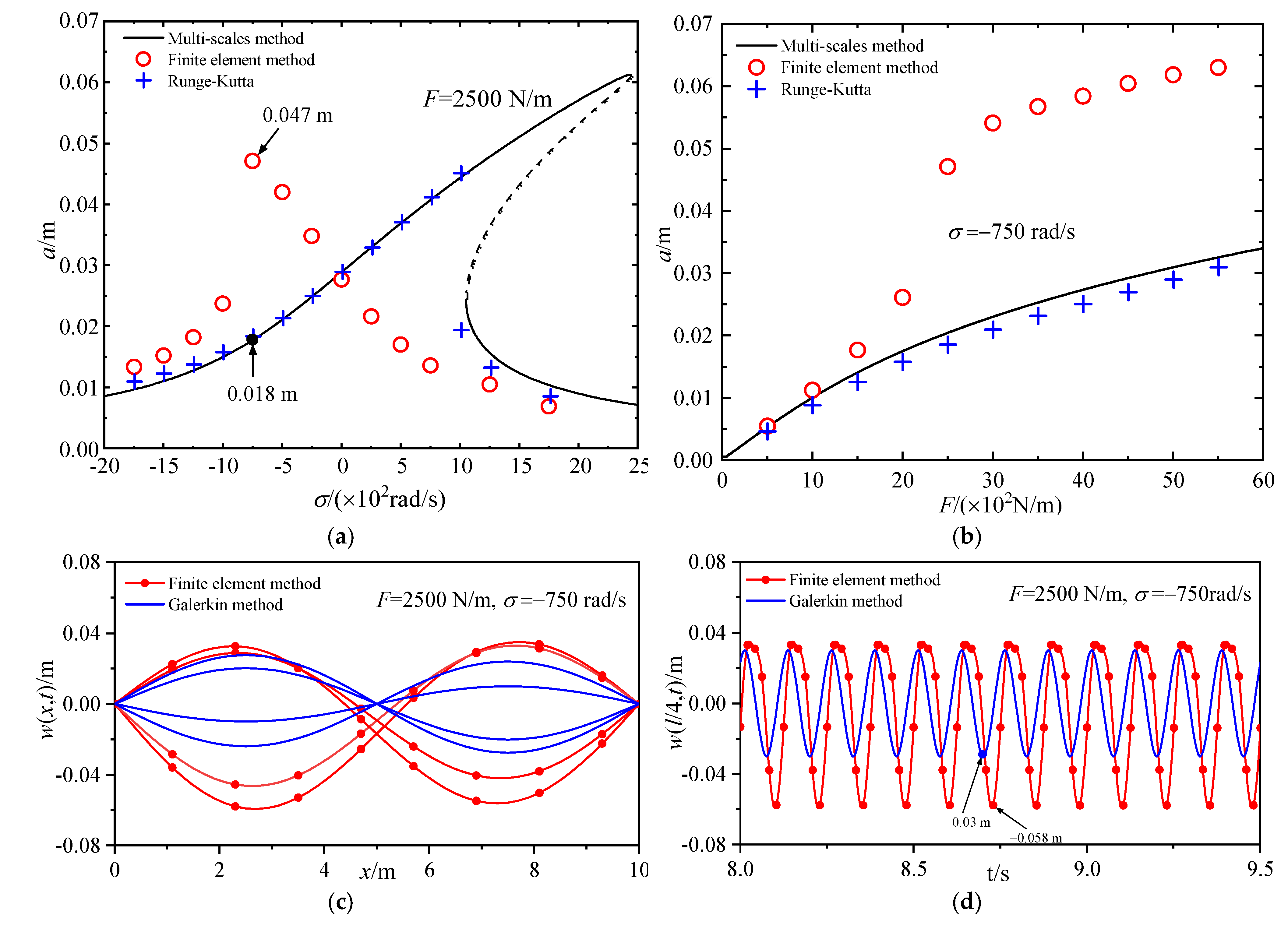
Next, we studied the second-order modal primary resonance. We also used the multiple scales method and the finite element method to solve the nonlinear response of hinged–hinged beams with the initial curvatures and . We obtained the amplitude–frequency response curves and the load–amplitude response curves of the second-order primary resonance of the beams, as shown in Figure 10 and Figure 11a,b. These figures represent the steady–state amplitude at 1/4 of beam length during steady–state motion. In the figure, “” is obtained by solving Equation (5) with the Runge–Kutta method.
Figure 10a shows that the amplitude–frequency response curves obtained by the two methods revealed hardening characteristics with a small initial curvature. However, there are quantitative differences in the steady–state amplitude. Figure 11a shows that the amplitude–frequency response curves obtained by the two methods demonstrate essential differences with the increase in the initial curvature of the beam. For example, the steady–state amplitude obtained with the Galerkin method is 0.018 m, whereas the steady–state amplitude obtained with the finite element method is 0.047 m at . Significant quantitative differences exist between the steady–state amplitudes of the two methods. Moreover, the amplitude–frequency response curves obtained by the Galerkin method have the hardening characteristic, while the amplitude–frequency response curve obtained with the finite element method has the softening characteristic. Figure 11b shows that there is no amplitude jump phenomenon in the load–amplitude response curve obtained by the Galerkin discrete method. On the contrary, the load–amplitude response curve with the finite element method indicates an amplitude jump phenomenon. Thus, these are qualitatively different dynamic behaviors obtained by the two methods. This phenomenon also indicates that the Galerkin method weakens the influence of the initial curvature and leads to erroneous results. Figure 11c shows the displacement of the second modal with time for the hinged–hinged beam with the initial curvature . Because the Galerkin single–mode discretization underestimates the effect of the square nonlinearity, the computed results do not display a significant drift phenomenon. On the contrary, the finite element method gives a significant drift phenomenon induced by the square nonlinearity. Figure 11d shows the time history of the second mode with the initial curvature under the primary resonance. In this case, there are obvious quantitative differences between the displacements obtained by the two methods. For example, the maximum displacement obtained by the Galerkin method is , whereas the maximum displacement obtained with the finite element method is . Moreover, since the drift phenomenon is caused by square nonlinearity, the vibration center of the beam is not at the position of . The above examples show that the Galerkin method with one modal may lead to erroneous results for nonlinear dynamic behaviors if a beam has a large initial curvature.
From the above discussion, we can find that the square nonlinear terms lead to different results with the two methods. Therefore, when nonlinear vibrations are analyzed for the structures without the initial curvature (e.g., strings, straight beams, and plates), one can use the Galerkin method to accurately obtain the dynamic behaviors of the structures. If the structures have initial curvature (e.g., buckled beam, shallow arch, sagged cable, and suspension bridges), the single–mode discretization obtained by the Galerkin method may lead to erroneous results. In these cases, the finite element method may be more suitable.
5. Conclusions
In the present study, we used the Galerkin method to obtain discrete equations, and the approximate analytical solutions for these discrete equations were obtained by the multiple scales method. Then, the full–scale accurate calculations of hinged–hinged beams were carried out using the finite element method. By comparing the results of these two methods, the following conclusions can be drawn.
- (1)
- If a beam does not have initial curvature, the amplitude–frequency response curves and the load–amplitude response curves calculated by the two methods are consistent. Therefore, one can use the Galerkin method to obtain the dynamic behaviors of straight beams accurately.
- (2)
- The initial curvature brings out a quadratic nonlinear term, and it has a softening effect on the amplitude–frequency response curve.
- (3)
- The mechanical behaviors of beams may change from hardening nonlinear behavior to softening nonlinear behavior with the increase in the initial curvature.
- (4)
- The square nonlinear terms drift the vibration’s center of the beams with the initial curvatures.
- (5)
- The Galerkin method may lead to a quantitative mistake at the single–mode discretization because the method underestimates the softening effect of the initial curvature.
Author Contributions
Conceptualization, K.H. and W.X.; methodology, K.H. and Y.Z.; software, Y.Z.; validation, Y.Z. and K.H.; formal analysis, Y.Z. and K.H.; resources, K.H.; data curation, W.X.; writing—original draft preparation, Y.Z.; writing—review and editing, K.H.; visualization, Y.Z.; supervision, K.H. and W.X.; project administration, W.X.; funding acquisition, K.H. All authors have read and agreed to the published version of the manuscript.
Funding
This work was supported by the National Natural Science Foundation of China (grant no. 12050001).
Data Availability Statement
No new data were created.
Conflicts of Interest
The authors declare no conflict of interest.
References
- Rega, G.; Lacarbonara, W.; Nayfeh, A.H. Reduction methods for nonlinear vibrations of spatially continuous systems with initial curvature. In Proceedings of the IUTAM Symposium on Recent Developments in Nonlinear Oscillations of Mechanical Systems, Hanoi, Vietnam, 2–5 March 1999; pp. 235–246. [Google Scholar]
- Kreider, W.; Nayfeh, A.H. Experimental investigation of single-mode responses in a fixed-fixed buckled beam. Nonlinear Dyn. 1998, 15, 155–177. [Google Scholar] [CrossRef]
- Tien, W.M.; Namachchivaya, N.S.; Bajaj, A.K. Non-linear dynamics of a shallow arch under periodic excitation–I. 1: 2 internal resonance. Int. J. Non-Linear Mech. 1994, 29, 349–366. [Google Scholar] [CrossRef]
- Huang, K.; Zhang, S.; Li, J.; Li, Z. Nonlocal nonlinear model of Bernoulli-Euler nanobeam with small initial curvature and its application to single-walled carbon nanotubes. Microsyst. Technol. 2019, 25, 4303–4310. [Google Scholar] [CrossRef]
- Qiao, W.; Guo, T.; Kang, H.; Zhao, Y. Softening–hardening transition in nonlinear structures with an initial curvature: A refined asymptotic analysis. Nonlinear Dyn. 2022, 107, 357–374. [Google Scholar] [CrossRef]
- Han, S.M.; Benaroya, H.; Wei, T. Dynamics of transversely vibrating beams using four engineering theories. J. Sound Vib. 1999, 225, 935–988. [Google Scholar] [CrossRef]
- Barari, A.; Kaliji, H.D.; Ghadimi, M.; Domairry, G. Non-linear vibration of Euler-Bernoulli beams. Lat. Am. J. Solids Struct. 2011, 8, 139–148. [Google Scholar] [CrossRef]
- Eltaher, M.A.; Khater, M.E.; Emam, S.A. A review on nonlocal elastic models for bending, buckling, vibrations, and wave propagation of nanoscale beams. Appl. Math. Model. 2016, 40, 4109–4128. [Google Scholar] [CrossRef]
- Younesian, D.; Hosseinkhani, A.; Askari, H.; Esmailzadeh, E. Elastic and viscoelastic foundations: A review on linear and nonlinear vibration modeling and Applications. Nonlinear Dyn. 2019, 97, 853–895. [Google Scholar] [CrossRef]
- Huang, K.; Feng, Q.; Qu, B. Bending aeroelastic instability of the structure of suspended cable-stayed beam. Nonlinear Dyn. 2017, 87, 2765–2778. [Google Scholar] [CrossRef]
- Huang, K.; Feng, Q.; Yin, Y. Nonlinear vibration of the coupled structure of suspended-cable-stayed beam–1:2 internal resonance. Acta Mech. Solida Sin. 2014, 27, 467–476. [Google Scholar] [CrossRef]
- Yao, J.; Huang, K.; Li, T. Vortex-Induced Nonlinear Bending Vibrations of Suspension Bridges with Static Wind Loads. Buildings 2023, 13, 2017. [Google Scholar] [CrossRef]
- Ansari, M.; Esmailzadeh, E.; Younesian, D. Internal-external resonance of beams on non-linear viscoelastic foundation traversed by moving load. Nonlinear Dyn. 2010, 61, 163–182. [Google Scholar] [CrossRef]
- Nayfeh, A.H. Reduced-order models of weakly nonlinear spatially continuous systems. Nonlinear Dyn. 1998, 16, 105–125. [Google Scholar] [CrossRef]
- Nayfeh, A.H. Introduction to Perturbation Techniques; Wiley-Interscience: New York, NY, USA, 1981. [Google Scholar]
- Ding, H.; Chen, L.-Q.; Yang, S.-P. Convergence of Galerkin truncation for dynamic response of finite beams on nonlinear foundations under a moving load. J. Sound Vib. 2012, 331, 2426–2442. [Google Scholar] [CrossRef]
- Chen, H.-Y.; Ding, H.; Li, S.-H.; Chen, L.-Q. The Scheme to Determine the Convergence Term of the Galerkin Method for Dynamic Analysis of Sandwich Plates on Nonlinear Foundations. Acta Mech. Solida Sin. 2021, 34, 1–11. [Google Scholar] [CrossRef]
- Chen, H.-Y.; Ding, H.; Li, S.-H.; Chen, L.-Q. Convergent term of the Galerkin truncation for dynamic response of sandwich beams on nonlinear foundations. J. Sound Vib. 2020, 483, 115514. [Google Scholar] [CrossRef]
- Lacarbonara, W. Direct treatment and discretizations of non-linear spatially continuous systems. J. Sound Vib. 1999, 221, 849–866. [Google Scholar] [CrossRef]
- Lacarbonara, W.; Nayfeh, A.H.; Kreider, W. Experimental validation of reduction methods for weakly nonlinear distributed-parameter systems: Analysis of a buckled beam. Nonlinear Dyn. 1998, 17, 95–117. [Google Scholar] [CrossRef]
- Rega, G.; Lacarbonara, W.; Nayfeh, A.H.; Chin, C.M. Multiple resonances in suspended cables: Direct versus reduced-order models. Int. J. Non-Linear Mech. 1999, 34, 901–924. [Google Scholar] [CrossRef]
- Pai, P.F.; Nayfeh, A.H. Fully nonlinear model of cables. AIAA J. 1992, 30, 2993–2996. [Google Scholar] [CrossRef]
- Arafat, H.N.; Nayfeh, A.H. Non-linear responses of suspended cables to primary resonance excitations. J. Sound Vib. 2003, 266, 325–354. [Google Scholar] [CrossRef]
- Pakdemirli, M.; Nayfeh, S.A.; Nayfeh, A.H. Analysis of one-to-one autoparametric resonances in cables–discretization vs. direct treatment. Nonlinear Dyn. 1995, 8, 65–83. [Google Scholar] [CrossRef]
- Rega, G. Nonlinear vibrations of suspended cable—Part II: Deterministic phenomena. Appl. Mech. Rev. 2004, 57, 479–514. [Google Scholar] [CrossRef]
- Nayfeh, A.H.; Nayfeh, J.F.; Mook, D.T. On methods for continuous systems with quadratic and cubic nonlinearities. Nonlinear Dyn. 1992, 3, 145–162. [Google Scholar] [CrossRef]
- Nayfeh, A.H.; Lacarbonara, W. On the discretization of distributed-parameter systems with quadratic and cubic nonlinearities. Nonlinear Dyn. 1997, 13, 203–220. [Google Scholar] [CrossRef]
- Ding, H.; Chen, L.-Q. Nonlinear vibration of a slightly curved beam with quasi-zero-stiffness isolators. Nonlinear Dyn. 2019, 95, 2367–2382. [Google Scholar] [CrossRef]
- Guo, T.D.; Rega, G. Direct and discretized perturbations revisited: A new error source interpretation, with application to moving boundary problem. Eur. J. Mech. A Solids 2020, 81, 103936. [Google Scholar] [CrossRef]
- Wang, S.; Wan, X.; Guo, M.; Qiao, H.; Zhang, N.; Ye, Q. Nonlinear Dynamic Analysis of the Wind–Train–Bridge System of a Long-Span Railway Suspension Truss Bridge. Buildings 2023, 13, 277. [Google Scholar] [CrossRef]
- Salenko, S.; Obukhovskiy, A.; Gosteev, Y.; Yashnov, A.; Lebedev, A. Strength, flexural rigidity and aerodynamic stability of fiberglass spans in pedestrian suspension bridge. Transp. Res. Procedia 2021, 54, 758–767. [Google Scholar] [CrossRef]
- Guan, Q.; Liu, L.; Gao, H.; Wang, Y.; Li, J. Research on Soft Flutter of 420m-Span Pedestrian Suspension Bridge and Its Aerodynamic Measures. Buildings 2022, 12, 1173. [Google Scholar] [CrossRef]
- Qi, D.; Chen, X.; Zhu, Y.; Zhang, Q. A new type of wind-resistance cable net for narrow suspension bridges and wind-resistance cable element for its calculation. Structures 2021, 33, 4243–4255. [Google Scholar] [CrossRef]
- Rodrigues, C.; Simões, F.M.F.; Pinto da Costa, A.; Froio, D.; Rizzi, E. Finite element dynamic analysis of beams on nonlinear elastic foundations under a moving oscillator. Eur. J. Mech. A Solids 2018, 68, 9–24. [Google Scholar] [CrossRef]
- Abdelrahman, A.A.; Nabawy, A.E.; Abdelhaleem, A.M.; Alieldin, S.S.; Eltaher, M.A. Nonlinear dynamics of viscoelastic flexible structural systems by finite element method. Eng. Comput. 2020, 38, 169–190. [Google Scholar] [CrossRef]
- Zhang, Y.; Teng, J.; Huang, J.; Zhou, K.; Huang, L. Free and Forced Vibration Analyses of Functionally Graded Graphene-Nanoplatelet-Reinforced Beams Based on the Finite Element Method. Materials 2022, 15, 6135. [Google Scholar] [CrossRef] [PubMed]
- Thompson, M.K.; Thompson, J.M. ANSYS Mechanical APDL for Finite Element Analysis; Elsevier Inc.: New York, NY, USA, 2017. [Google Scholar]
- Alawadhi, E.M. Finite Element Simulations Using ANSYS; CRC Press: Panama City, FL, USA, 2009. [Google Scholar]
- Lee, Y.Y.; Su, R.K.L.; Hui, C.K. The effect of the modal energy transfer on the sound radiation and vibration of a curved panel: Theory and experiment. J. Sound Vib. 2009, 324, 1003–1015. [Google Scholar] [CrossRef]
- Nayfeh, A.H.; Mook, D.T. Nonlinear Oscillations; John Wiley & Sons: New York, NY, USA, 2008. [Google Scholar]
- Bathe, K.J. Finite Element Procedures; Prentice Hall Inc.: Upper Saddle River, NJ, USA, 1996. [Google Scholar]
Figure 1.
Schematic diagram of a hinged–hinged beam.
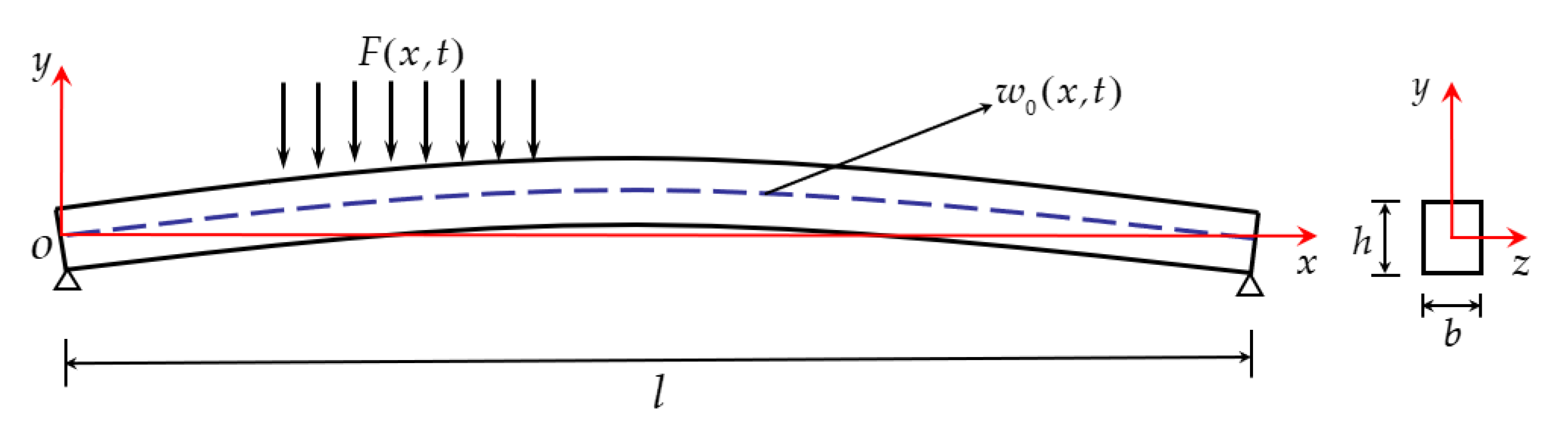
Figure 2.
Finite element model of the hinged–hinged beam.
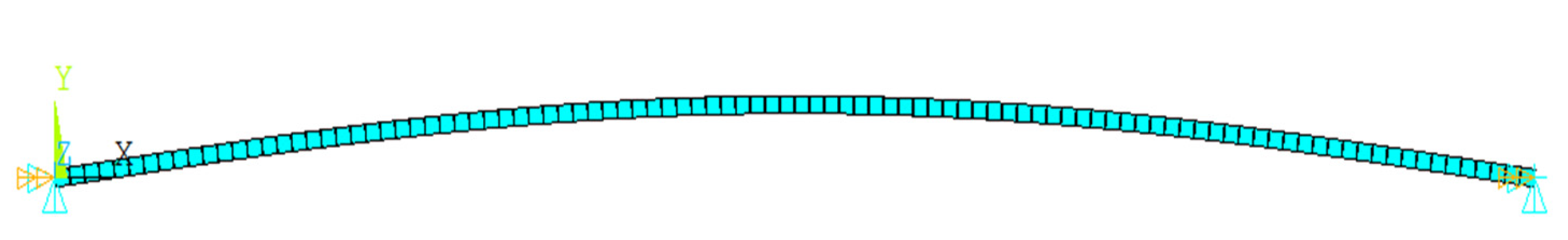
Figure 3.
Amplitude–frequency response curves: (a) primary resonance of the first-order modal and (b) primary resonance of the second-order modal.
Figure 3.
Amplitude–frequency response curves: (a) primary resonance of the first-order modal and (b) primary resonance of the second-order modal.
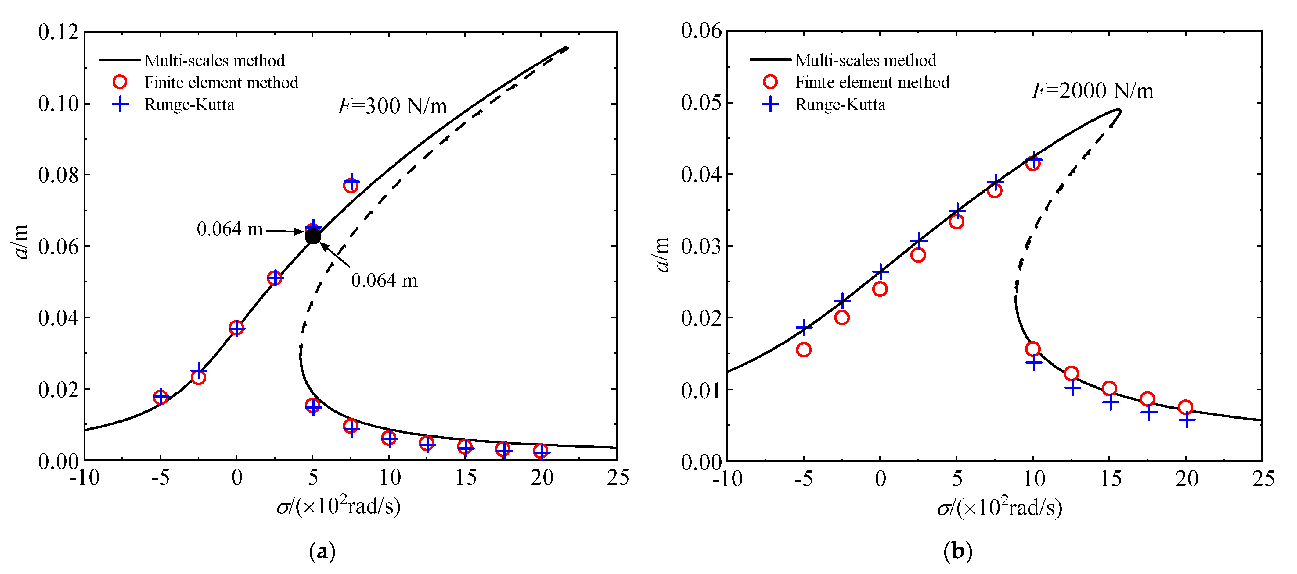
Figure 4.
Load–amplitude response curves: (a) primary resonance of the first-order modal and (b) primary resonance of the second-order modal.
Figure 4.
Load–amplitude response curves: (a) primary resonance of the first-order modal and (b) primary resonance of the second-order modal.
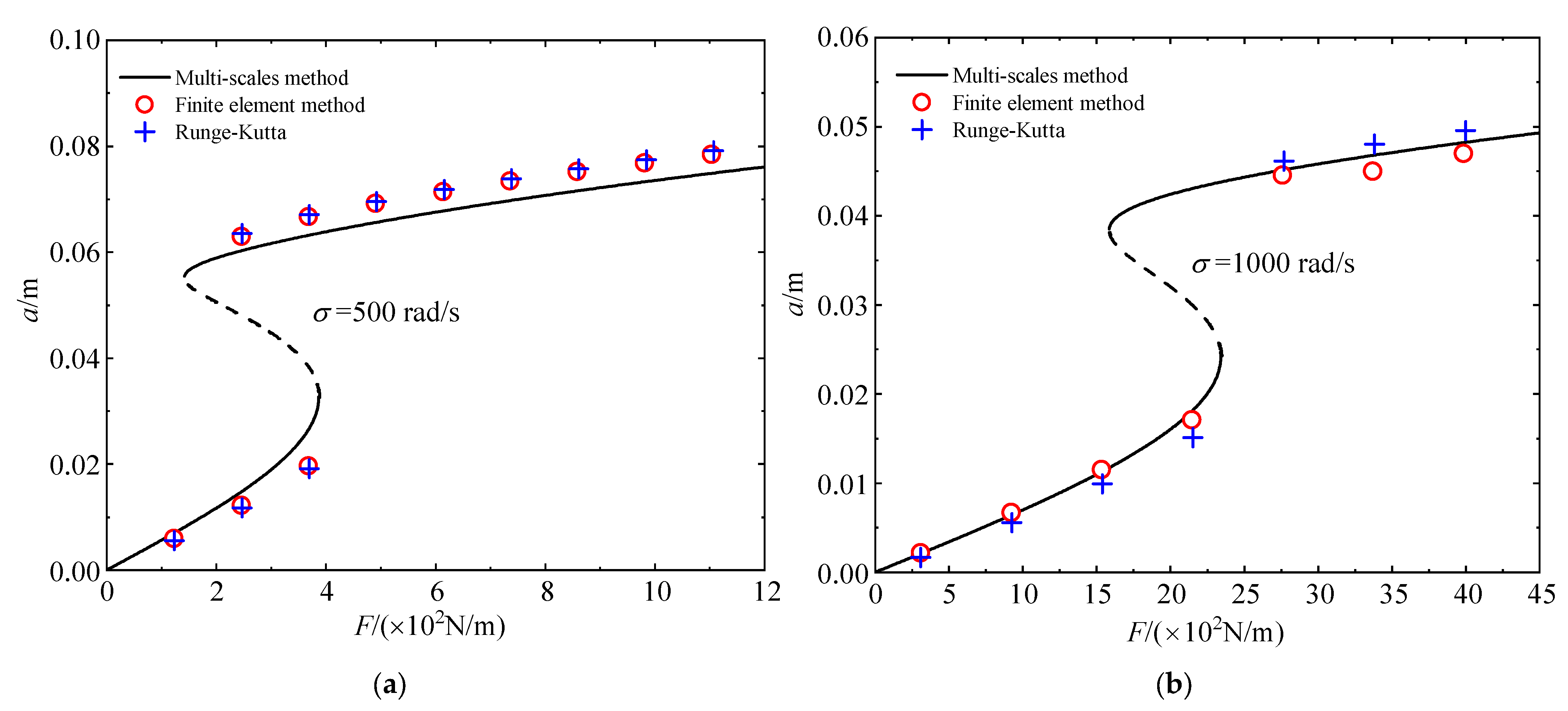
Figure 5.
Displacements at different instants: (a) primary resonance of the first-order modal and (b) primary resonance of the second-order modal.
Figure 5.
Displacements at different instants: (a) primary resonance of the first-order modal and (b) primary resonance of the second-order modal.
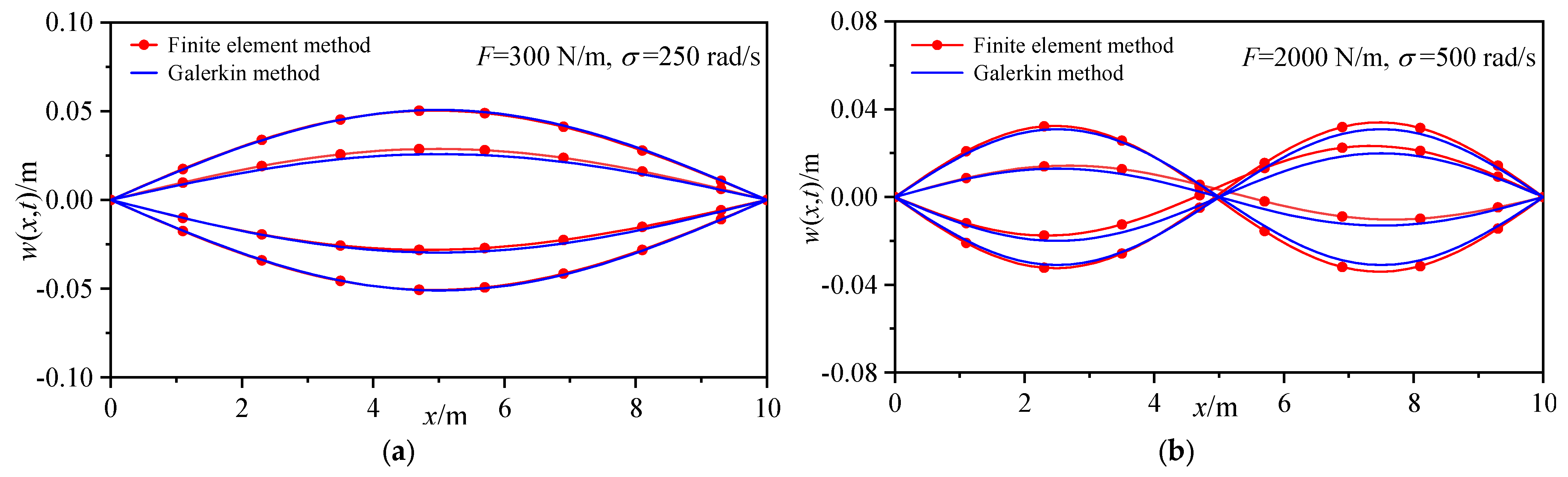
Figure 6.
Time history diagrams during steady–state motion: (a) primary resonance of the first-order modal and (b) primary resonance of the second-order modal.
Figure 6.
Time history diagrams during steady–state motion: (a) primary resonance of the first-order modal and (b) primary resonance of the second-order modal.
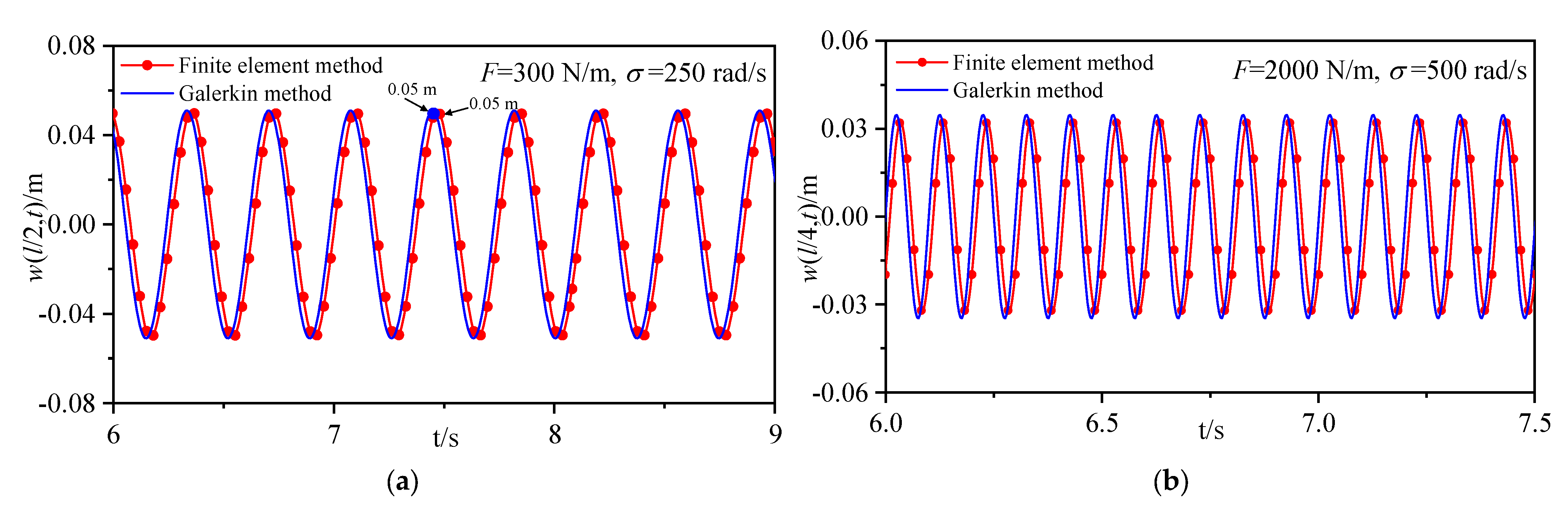
Figure 7.
First–mode primary resonance for (a) amplitude–frequency response curve and (b) load–amplitude response curve.
Figure 7.
First–mode primary resonance for (a) amplitude–frequency response curve and (b) load–amplitude response curve.
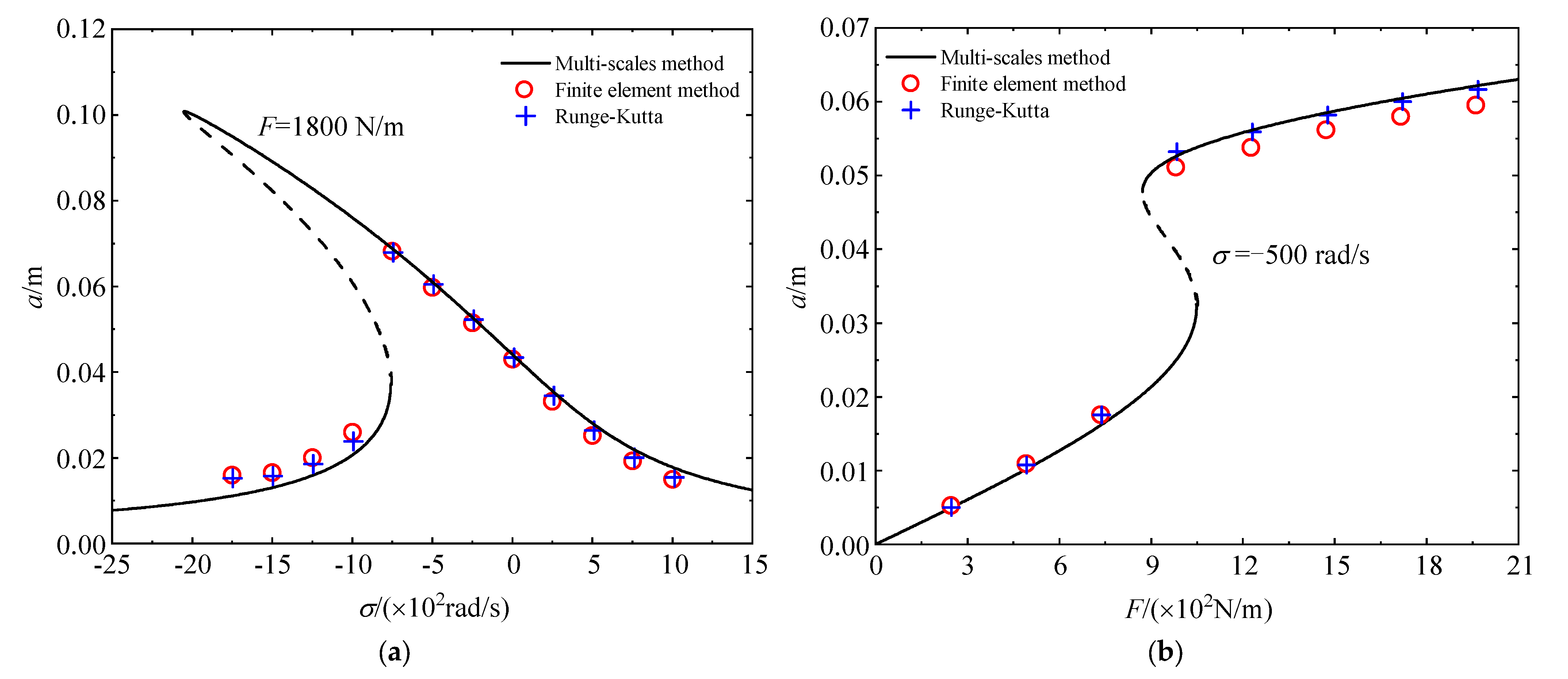
Figure 8.
First–mode primary resonance for (a) amplitude–frequency response curve and (b) load–amplitude response curve.
Figure 8.
First–mode primary resonance for (a) amplitude–frequency response curve and (b) load–amplitude response curve.
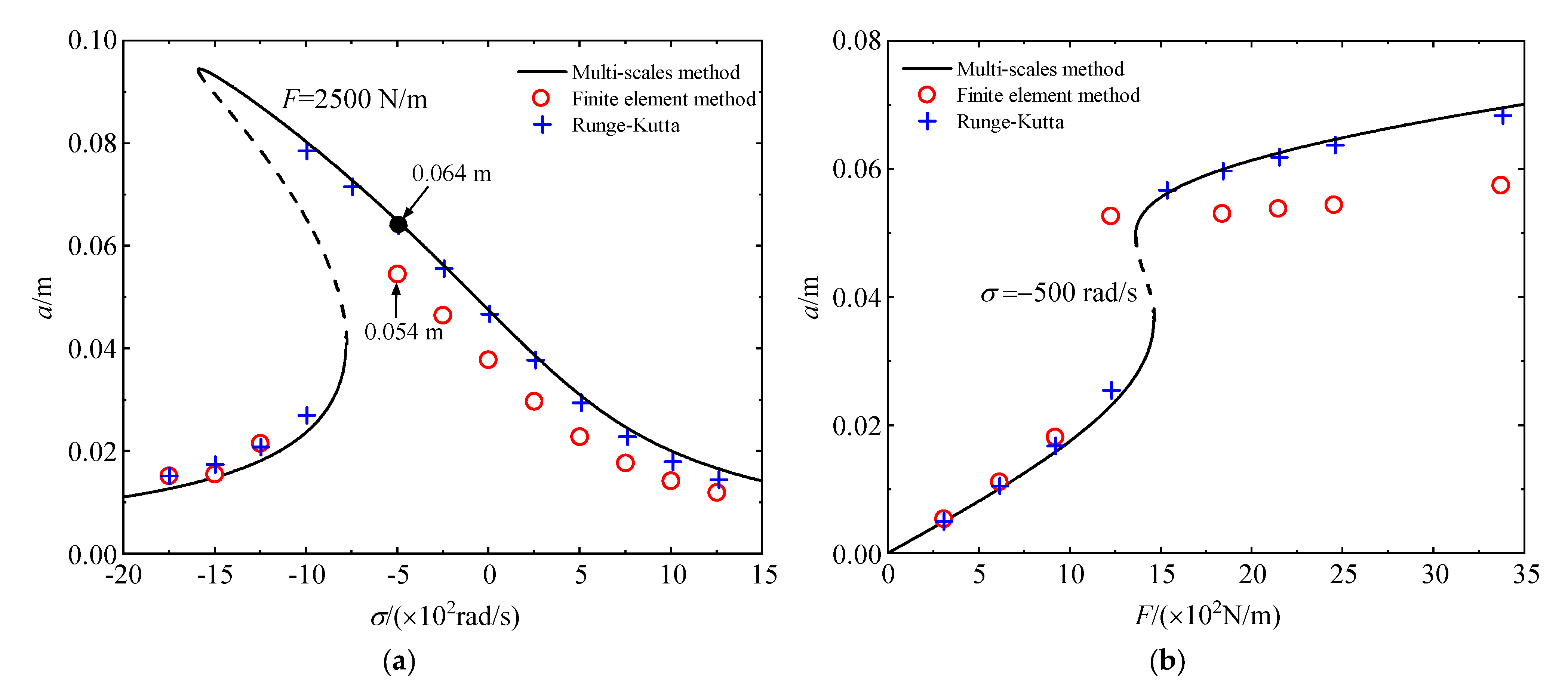
Figure 9.
First–mode primary resonance for (a) amplitude–frequency response curve, (b) load–amplitude response curve, (c) in–plane displacement of the first–mode solution at different instants, and (d) time history diagram.
Figure 9.
First–mode primary resonance for (a) amplitude–frequency response curve, (b) load–amplitude response curve, (c) in–plane displacement of the first–mode solution at different instants, and (d) time history diagram.

Figure 10.
Second–mode primary resonance for (a) amplitude–frequency response curve and (b) load–amplitude response curve.
Figure 10.
Second–mode primary resonance for (a) amplitude–frequency response curve and (b) load–amplitude response curve.

Figure 11.
Second–mode primary resonance for (a) amplitude–frequency response curve, (b) load–amplitude response curve, (c) in–plane displacements of the second mode at different instants, and (d) time history diagram.
Figure 11.
Second–mode primary resonance for (a) amplitude–frequency response curve, (b) load–amplitude response curve, (c) in–plane displacements of the second mode at different instants, and (d) time history diagram.

Table 1.
Physical and geometrical parameters of the beam.
| 78 | 10 | 0.1 | 0.1 | 200 | 0.05 |
Disclaimer/Publisher’s Note: The statements, opinions and data contained in all publications are solely those of the individual author(s) and contributor(s) and not of MDPI and/or the editor(s). MDPI and/or the editor(s) disclaim responsibility for any injury to people or property resulting from any ideas, methods, instructions or products referred to in the content. |
© 2023 by the authors. Licensee MDPI, Basel, Switzerland. This article is an open access article distributed under the terms and conditions of the Creative Commons Attribution (CC BY) license (https://creativecommons.org/licenses/by/4.0/).
Share and Cite
MDPI and ACS Style
Zhang, Y.; Huang, K.; Xu, W. Validity of Galerkin Method at Beam’s Nonlinear Vibrations of the Single Mode with the Initial Curvature. Buildings 2023, 13, 2645. https://doi.org/10.3390/buildings13102645
AMA Style
Zhang Y, Huang K, Xu W. Validity of Galerkin Method at Beam’s Nonlinear Vibrations of the Single Mode with the Initial Curvature. Buildings. 2023; 13(10):2645. https://doi.org/10.3390/buildings13102645
Chicago/Turabian StyleZhang, Yunbo, Kun Huang, and Wei Xu. 2023. "Validity of Galerkin Method at Beam’s Nonlinear Vibrations of the Single Mode with the Initial Curvature" Buildings 13, no. 10: 2645. https://doi.org/10.3390/buildings13102645
Note that from the first issue of 2016, this journal uses article numbers instead of page numbers. See further details here.