Pollutant Diffusion in an Infectious Disease Hospital with Different Thermal Conditions

1
Changsha University of Science and Technology, Changsha 410076, China
2
China Construction Fifth Engineering Bureau Co., Ltd., Changsha 410004, China
3
Hubei Business College, Wuhan 430079, China
4
Changsha University, Changsha 410012, China
*
Author to whom correspondence should be addressed.
Buildings 2024, 14(4), 1185; https://doi.org/10.3390/buildings14041185
Submission received: 6 March 2024
/
Revised: 16 April 2024
/
Accepted: 17 April 2024
/
Published: 22 April 2024
(This article belongs to the Section Building Energy, Physics, Environment, and Systems)
Abstract
:In recent years, the outbreak of infectious diseases has highlighted the need for improved planning of hospital buildings. Traditional planning for infectious disease hospitals only considers the impact of wind and pollutant diffusion, without analysing pollutant diffusion under different thermal conditions. To reveal the distribution of pollutants in infectious disease hospitals under different thermal conditions, this study conducted wind tunnel tests and numerical analyses of pollutant diffusion in the environment surrounding an infectious disease hospital in Changsha, China. The results show that the pollutant concentration mainly depends on the local wind speed. In the range of Rb = −1.25 to 1.25, the concentration of pollutants was mainly affected by the disturbance of the flow field in areas with rough surfaces, where the effect of the thermal stability of the atmosphere on pollutant diffusion was relatively small. However, in relatively flat regions, the thermal stability of the atmosphere played a significant role in pollutant diffusion around the buildings.
1. Introduction
Environmental problems caused by industrial waste gases, urban heat islands, and aerosol viruses have seriously threatened human health worldwide. In the past decades, many scholars have studied the diffusion of pollutants in the environment surrounding buildings [1,2,3,4]. The research methods mainly include wind tunnel tests [5,6], numerical simulations [7,8,9,10], and field measurements [11]. In 2011, Liu et al. (2011) analysed the wind environment in a residential community using field measurements, considering the influence of thermal conditions on the wind environment in detail [12]. Although the field measurement method can directly obtain flow field information, it has not been widely applied owing to the associated expense and difficulty of maintaining the measurement devices. Nardecchia et al. (2016) used numerical simulation methods to study the flow field around buildings, considering different thermal conditions [13], and Xie et al. (2006) used numerical simulations to study the effects of solar radiation on the diffusion of urban street valley pollutants [14]. However, owing to the uncertainty of the calculation parameters, numerical simulations often require wind tunnel tests and field measurements for verification [15,16]. With the rapid development of experimental technology, research on pollutant dispersion has developed rapidly. Ou et al. (2003) found that the concentration of pollutants is mainly affected by the inflow velocity [17]. Hajra and Stathopoulos (2012) reported that the height and spacing of downstream buildings are critical parameters influencing pollutant diffusion [18]. Gousseau et al. (2011) conducted a case study of a Montreal, Canada, community, analysing the pollutant diffusion near the ground to compare the results with those of numerical simulations [19]. Liu et al. (2010) used a wind tunnel test to study pollutant diffusion in the environment surrounding a typical building in Hong Kong and analysed the impact of the windows on the results [20]. To date, most pollutant studies have concentrated on urban street valleys and urban communities [21,22,23]; there is a notable lack of analysis of viral diffusion in the environment surrounding hospitals. During the 2003 outbreak of severe acute respiratory syndrome (SARS), the virus that is responsible for SARS was found on the windows and exterior walls of uninfected residents’ homes [9,24], indicating that it was able to diffuse into the air. Niu and Tung (2008) and Gao et al. (2008) reported that the virus transmission rate from a standard room to adjacent upper rooms was 7%. Later [25,26], Liu et al. (2010) and Wang et al. (2010) used wind tunnel tests to determine that the virus can spread in the horizontal and vertical directions around a building [27].
Although many researchers have used wind tunnel experiments to study pollutant dispersion, the effects of thermal conditions are rarely considered, because it can be challenging to apply the similarity ratio to such effects in wind tunnel tests. Chao et al. (2020) studied pollutant dispersion using simple standard models, considering the effect of the thermal condition, and pointed out that high buoyancy can effectively reduce the concentration of pollutants on the windows of a building [28]. However, different thermal conditions were not reflected in Chao’s study. Meanwhile, owing to the limitations of the experimental resolution, it has been difficult to determine the mechanism by which viruses spread. Therefore, numerical simulations are required to analyse the spread of viruses among buildings. Unstable and neutral atmospheres have primarily been studied [29,30,31,32,33,34,35,36,37], while very few studies have dealt with an atmosphere under stable conditions [38,39,40,41,42], and studies targeting the diffusion of viral pollutants under atmospheric conditions owing to thermal effects have not been reported to date.
Therefore, to address the limitations of previous research, this study conducted a comprehensive wind tunnel test and numerical analysis of pollutant diffusion in the environment surrounding an infectious disease hospital in Changsha, China, taking into account various thermal conditions. The paper is structured as follows: Section 2 briefly introduces the wind tunnel test setup, while Section 3 presents a detailed analysis of the experiment. Section 4 analyses the numerical simulation of the wind field and pollutant dispersion mechanism. Section 5 presents the conclusions.
2. Introduction of the Wind Tunnel Test
2.1. Wind Tunnel Test Setup
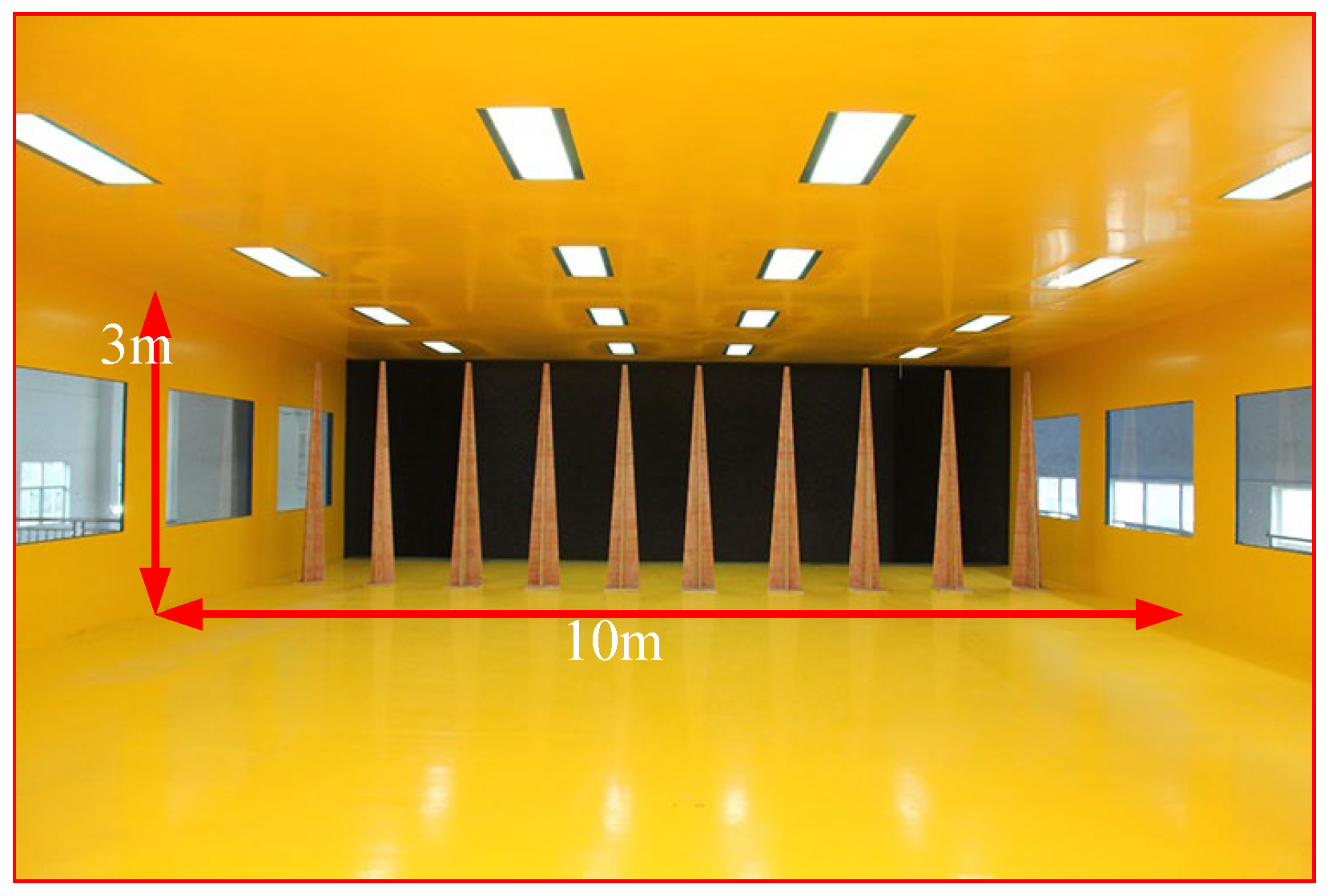
The wind tunnel tests were carried out at the Wind Engineering and Wind Environment Research Centre of Changsha University of Science and Technology. Figure 1 shows the cross-section of the wind tunnel, which is 10.0 m wide and 3.0 m high. The wind speed can be adjusted from 1.0 m/s to 18.0 m/s. To ensure the stability and reliability of the wind at low speeds, a system of variable angle fan blades was used.
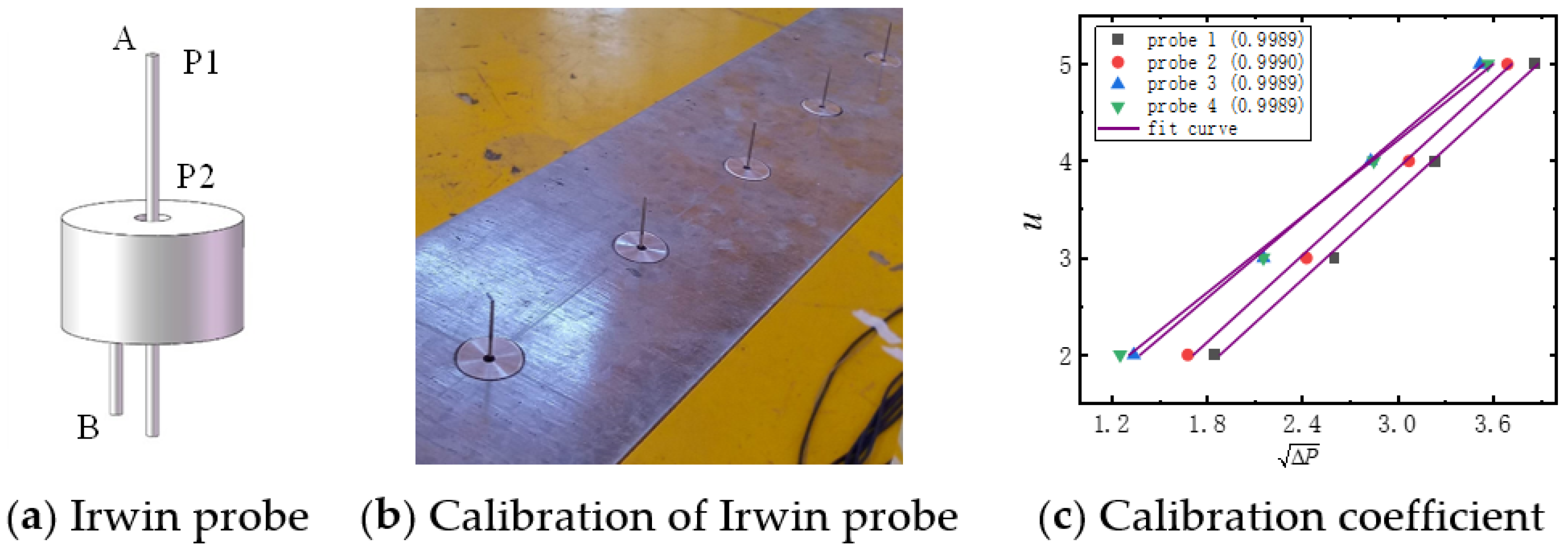
During the test, the horizontal pedestrian-level wind (PLW) velocities were measured using Irwin probes. A schematic diagram of an Irwin probe is shown in Figure 2a, in which the pressure value at the top is labelled P1 and the pressure value at the groove part is labelled P2. According to the Irwin probe theory [43,44,45], the relationship between the probe-measured pressure and the applied wind velocity can be expressed as follows:
where is the wind velocity at the test height, and and are calibration coefficients.
Prior to the test, the probe device setup shown in Figure 2b was used to calibrate the Irwin probe, with the resulting calibration coefficients being shown in Figure 2c. During the test, an electronic pressure scan valve was used to measure the wind pressure at a frequency of 350 Hz for 1 min, and a Cobra probe was used to measure the wind profile by the three-dimensional moving frame.
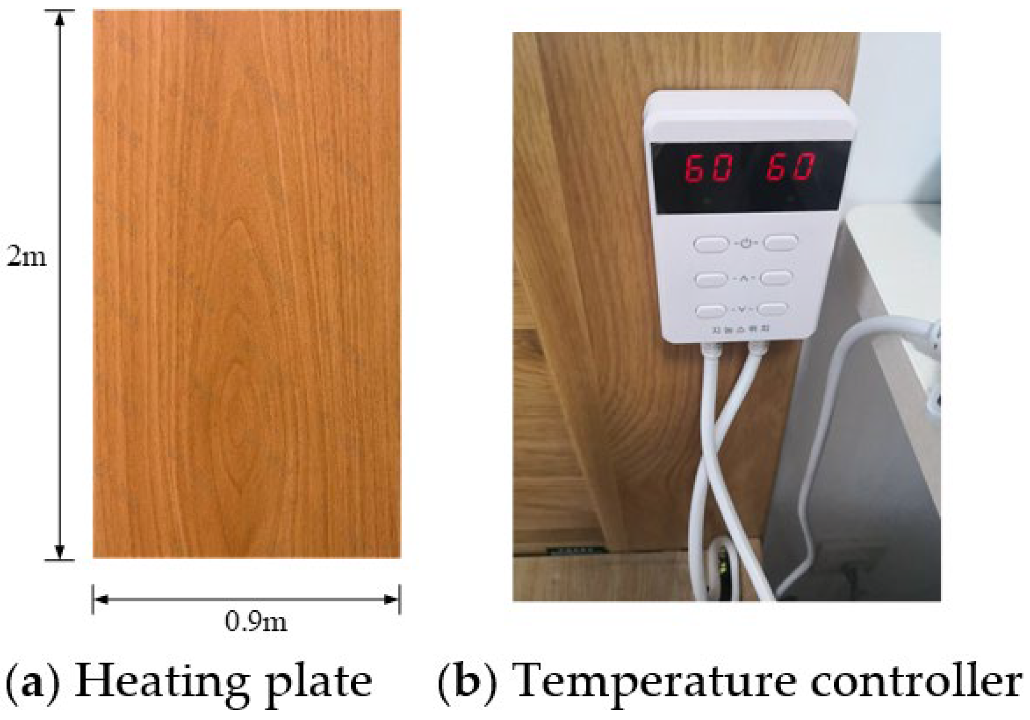
The temperature was adjusted using carbon fibre heating plates, as shown in Figure 3. The size of the plate is 2 m × 0.9 m, and 20 plates were employed to provide the temperate. The temperature range of the plate ranged from 0 °C to 60 °C. The temperature of the carbon fibre heating plate was calibrated within an accuracy margin of ±1 °C.
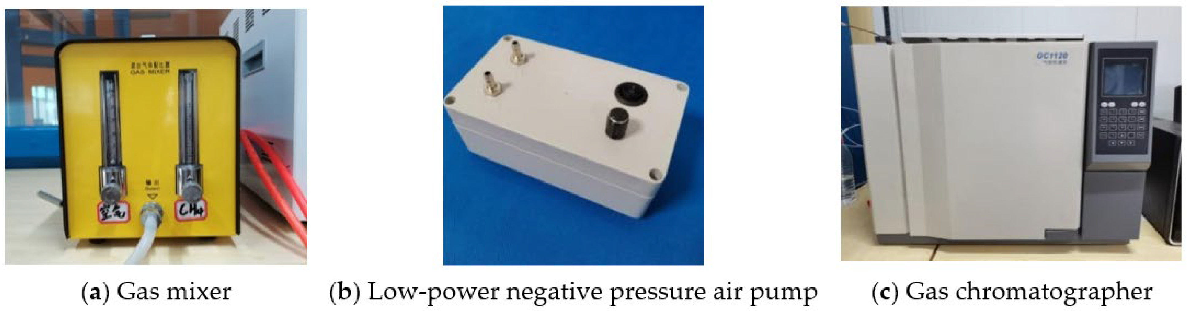
The wind tunnel tests used methane (CH4) as a tracer gas to simulate pollutant diffusion. The methane was emitted from a gas mixer (Figure 4a) located in front of the target building group. A low-power negative pressure air pump (Figure 4b) was employed to collect the air to the air bags, and gas chromatography (Figure 4c) was adopted to analyse the tracer gas concentration. The mixing ratio of tracer gas to air was 1:9. The overall schematic of the wind tunnel test is shown in Figure 5.
2.2. Similarity Conditions of Wind Tunnel Test
Wind tunnel tests must strictly control the similarity ratios of the parameters so that the test results can be scaled to a natural flow. When the simulation region is smaller than 5 km, Rossby (Ro) can be ignored. Because air is the medium of both the test model and the natural flow, Péclet (Pe) and Schmidt (Sc) can also be ignored. The value of Re for the target building is defined as
where is the density of air, u is the velocity of the incoming flow, L is the model building’s length, and μ is the viscous coefficient of air.
It is difficult to satisfy the similarity of Re in a wind tunnel test. Fortunately, the typical sections of the target building are primarily rectangular, and their flow field characteristics do not change significantly over a wide range of Re values. Lateb et al. (2013) pointed out that when the Re of a wind tunnel model is greater than the critical Re, the turbulent structure of the boundary layer can be fully developed, and the effect of Re on the field flow can be ignored [10]. The critical Re, defined as ReH, is approximately 1.1 × 10⁴; in the present study, Re was approximately 2 × 10⁵, which means that the flow field in the wind tunnel test had little effect on Re. To effectively consider the influence of the ground temperature effect on the flow field, the Rb (Richardson number) is applied to represent the intensity of the thermal condition owing to the ground surface temperature, and is defined as
where g is the gravitational acceleration, h0 is the model height, and Tb is the temperature at the top of the building. Ts is the temperature at the ground surface. u0 is the wind velocity at h0, and T0 is the average absolute temperature.
2.3. Geometric Model and Test Cases
An infectious disease hospital in Changsha was used as the case study, with a model scale ratio of 1:200, and the blockage rate was 2% in the wind tunnel test. A uniform wind velocity of 1.2 m/s was set as the inlet velocity. In all tests, 110 Irwin probes were used to capture the average wind velocity at a height of 2 m. During the test, the heating plate was used to create four different thermal conditions (Rb = 0, −0.17, −0.28, and −0.38) for the investigation of the building flow field distribution. Simultaneously, the flow field and pollutant concentration field for different building orientations were analysed in detail. The specific cases investigated in the wind tunnel tests are listed in Table 1. The hospital model and pollutant concentration monitoring points are shown in Figure 6.
3. Experimental Results and Discussions
3.1. Wind Field
As discussed in Section 2.2, the dimensionless distribution of a flow field does not change with the wind velocity within a specific range of Re. The mean wind velocity ratio (MVR) is defined as the ratio of the PLW velocity ui at monitoring point I to the inflow velocity u0 at the same height and can be expressed as follows:
The MVR values corresponding to different thermal conditions are compared for the prevailing wind direction in Figure 7, in which it can be observed that Rb mainly affected MVR values below 0.6. When the MVR was greater than 0.6, the thermal effect had little impact on the wind field distribution.
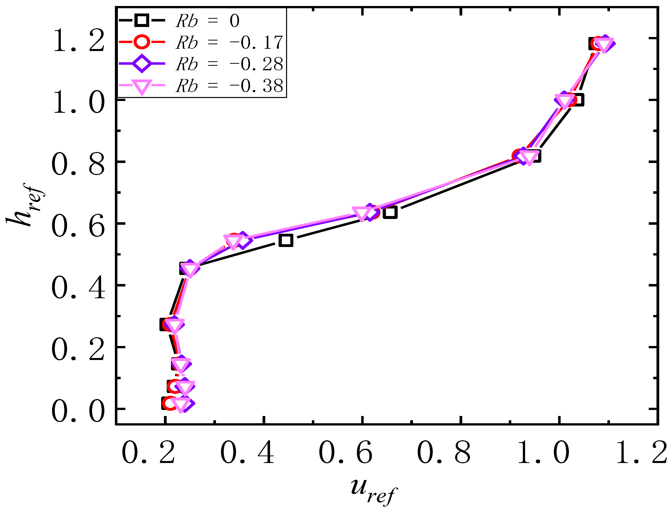
To determine the effect of the thermal condition on the wind profile, a detailed analysis of the wind profile at point 16 (shown in Figure 6b) was carried out, and the resulting longitudinal-direction dimensionless wind profile is shown in Figure 8, where href = h/h0, uref = u/u0, h0 = 0.5 m, and u0 is the wind speed at the height h0. It can be observed in Figure 8 that the shear wind height at point 16 was approximately 0.5href, and the average wind velocity at the shear height was approximately 0.2uref. Meanwhile, it can also be observed that the wind speed sharply increased between the heights [0.5href, 0.8href]. Generally speaking, the influence of Rb on the downwind wind speed was small, the main reason for this being that it was limited by the conditions of the wind tunnel test, and the degree of atmospheric instability was relatively low, so that the wind speed did not change significantly.
3.2. Tracer Gas Concentration Field
Methane was used as the tracer gas in this study. The methane concentration profile at point 16 was measured during the wind tunnel tests, and the results are shown in Figure 9, in which Cref = C/C0, where C is the methane concentration at the measurement height and C0 is the methane concentration at the roof height. It can be observed in the figure that the methane concentration was relatively high near the ground but decreased to nearly zero at the height of the building roof as the fresh air moving above the building diluted the tracer gas. The figure also shows that the methane concentration value in the height range [0.65href, 1.2href] exhibited no noticeable change according to the Rb value. However, when the height was less than 0.65href, the concentration of methane initially increased and then decreased as the Rb value increased. The methane concentration exhibited its maximum value at Rb = −0.28. Overall, with the increase in the Rb number, the concentration of pollutants did not change monotonously. The main reasons are that the monitoring point is located in the building complex, the surface wind field is disordered, and the pollutant concentration is affected by the coupling effect of the complex wind field and thermal effects.
3.3. Impact of Building Orientation on Tracer Gas Diffusion
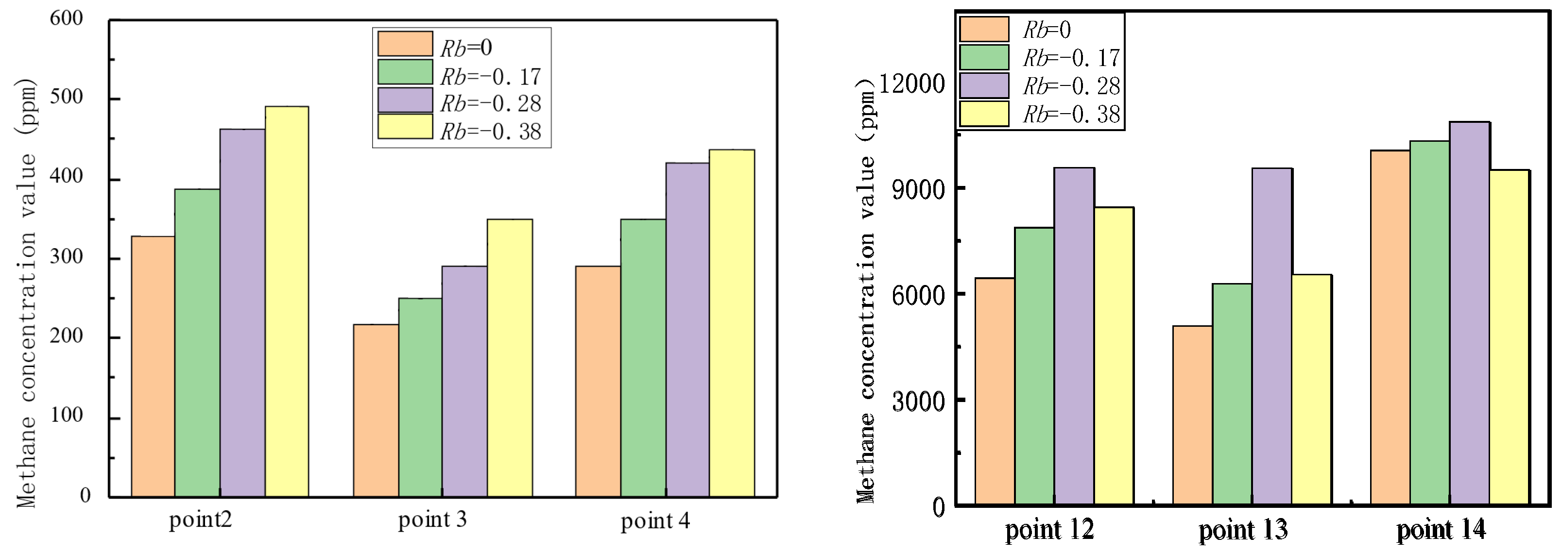
To analyse the effect of different building layouts on pollutant concentrations, four different building orientations were applied to building 3, as shown in Figure 10, to obtain the resulting distributions of the methane tracer gas around the building according to the thermal condition, as shown in Figure 11. It can be observed in the figures that under 0°, the wind speed at point 16 was relatively low, but the methane concentration was the highest, indicating that pollutant concentration is inversely proportional to wind speed. Figure 11 also shows that the methane concentrations at points 12 to 14 were relatively large when Rb = −0.28, indicating that pollutants are not easily diffused under this condition, which is consistent with the results shown in Figure 9. Figure 12 shows the pollutant concentration profiles at point 17, which indicate that pollutant concentrations decrease with increasing heights. For a building orientation angle of 45°, the methane concentrations decreased faster than for the other orientations, primarily because at 45°, the ventilation corridor of the building structure was aligned with the dominant wind direction, promoting pollutant diffusion. In addition, Figure 11 shows the concentration distribution of measuring points 12, 13, and 14. It is found from the figure that the concentration of pollutants in this area was significantly higher than those of measuring points 2, 3, and 4, mainly because these measuring points are affected by surface obstacles. The wind speed was relatively low, and the methane concentration at measuring point 13 was lower than those of measuring points 12 and 14. The reason is that measuring point 13 is located in the ventilation corridor of the building, and the accelerated flow field is conducive to the diffusion of pollutants. Therefore, it is recommended that architectural planners lay out buildings so that ventilation corridors align with the predominant wind directions in order to maximise the pollutant diffusion.
4. Numerical Simulation of Wind Environment and Pollutant Diffusion
4.1. Control Equation and Turbulence Model
The Reynolds-averaged Navier–Stokes (RANS) equations are commonly used to model turbulence in wind environment simulations of actual residential areas. The shear stress transport (SST) k–ω turbulence model is an approximation of the RANS equations that is suitable for calculating the inverse pressure gradient and separated flow and has been widely used in recent years. The SST control equation can be expressed as
where xj represents the spatial coordinates of points (i, j = 1, 2, 3); t is the time; ρ is the air density; υ is the air viscosity coefficient; p is the air pressure; k and ω are the turbulent kinetic energy and turbulent kinetic energy dissipation rate, respectively; Г, Гk, and Гω are the effective diffusion coefficients for the velocity, k, and ω, respectively; and Gω are the generation terms of k and ω, respectively, and Yk, Yω are the corresponding dissipation terms; Dω is the cross-diffusion of ω; and Si, Sk, and Sω are self-defining terms.
In this study, pollutant diffusion was modelled by the component transport mode, chemical reactions between components were not considered in the simulation process, and the mass conservation equation was applied as follows:
where cs is the volume concentration of the component, ρcs is the mass concentration, Ds is the diffusion coefficient, and Ss is the production rate.
4.2. Calculation Domain and Grids
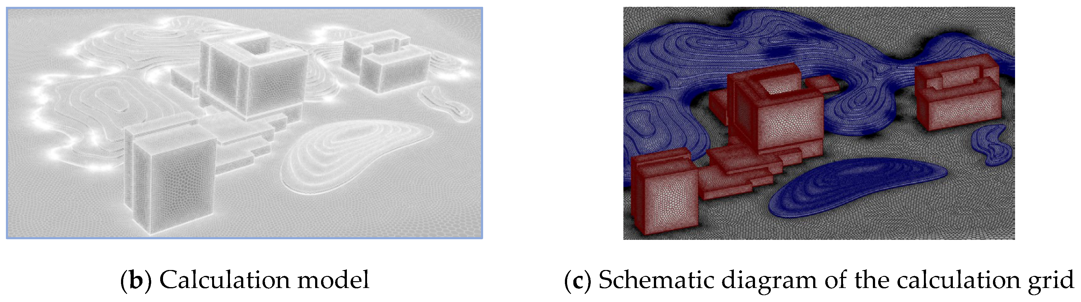
The numerical model corresponding to the wind tunnel tests is shown in Figure 13a. FLUENT software was used for the numerical simulations in this paper [46]. The domain size and meshes used in this study were determined according to the Architectural Institute of Japan guidelines. The inlet was set at a distance of 6H (H is the building height) from the building centre, the outlet was set at a distance of 22H from the building, and the height of the calculation domain was 6H. The coordinate origin was set at the bottom centre of the building model. A 7.8-million-cell polyhedral mesh was used in this study and is shown in Figure 13b. In the horizontal direction, local meshes were refined near the building and wake areas to accurately capture the changes in the flow fields around the building model. The mesh size near the surface was 0.0025 m, the largest mesh size in the horizontal direction was 0.3 m, and the stretching ratio was 1.2. The y+ of the mesh that was attached to the building surface and ground was less than 1. Three mesh systems with different resolutions were evaluated to verify grid independence, and the mesh system adopted in the present study met the grid independence requirements.
4.3. Boundary Condition and Parameter Setting
All calculation cases were performed on a workstation with a 12-core 24-thread Intel Core i9-7980 XE processor. The finite-volume method and the second-order central difference scheme were used for the convective and viscous terms, and a second-order implicit scheme was employed for the unsteady term. The semi-implicit pressure-linked equations (SIMPLE) algorithm was used to solve the discretised equations, as shown by Ferziger and Peric (2002) [47]. The computational parameters and details of the boundary conditions are presented in Table 2.
4.4. Results and Discussion
4.4.1. Validation of Numerical Simulation
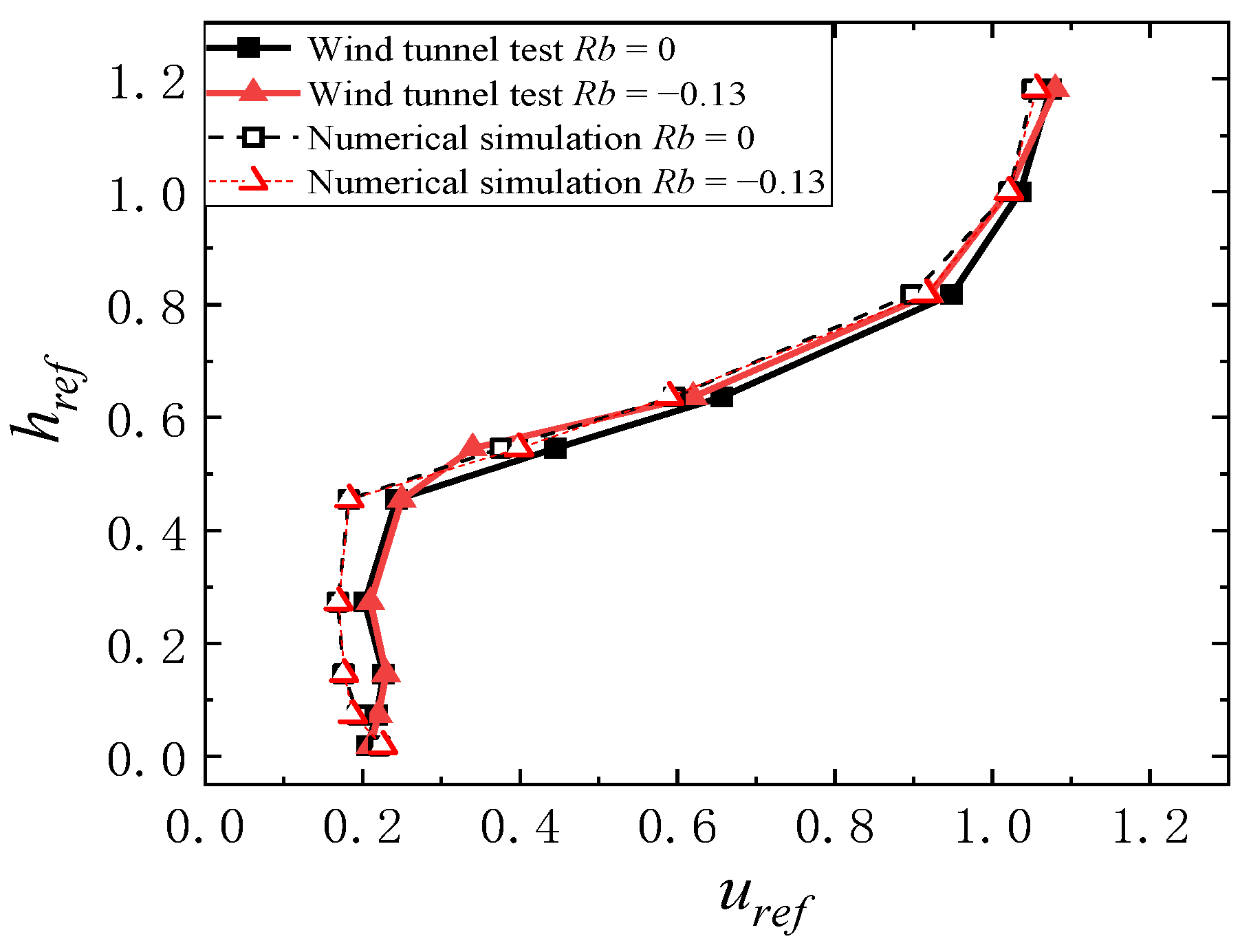
To verify the simulation results, the simulated wind profile at point 16 on the hospital building was compared with the experimental results, as shown in Figure 14. It can be seen that the numerical simulation of the longitudinal velocity was generally in good agreement with the experimental results.
Similarly, the methane tracer gas concentrations that were obtained by the numerical simulation were compared with those obtained in the wind tunnel test along the height of the building at point 16, as shown in Figure 15. The numerical simulation results were found to be consistent with the experimental results. Near the ground, the tracer gas concentration was considerably higher in the numerical simulation than in the wind tunnel test, primarily because the wind speed was relatively high in the wind tunnel test, promoting tracer gas diffusion. The general agreement of the wind and methane tracer gas concentration profiles therefore confirmed the accuracy of the numerical simulation.
4.4.2. Distribution of Wind Field and Temperature Field
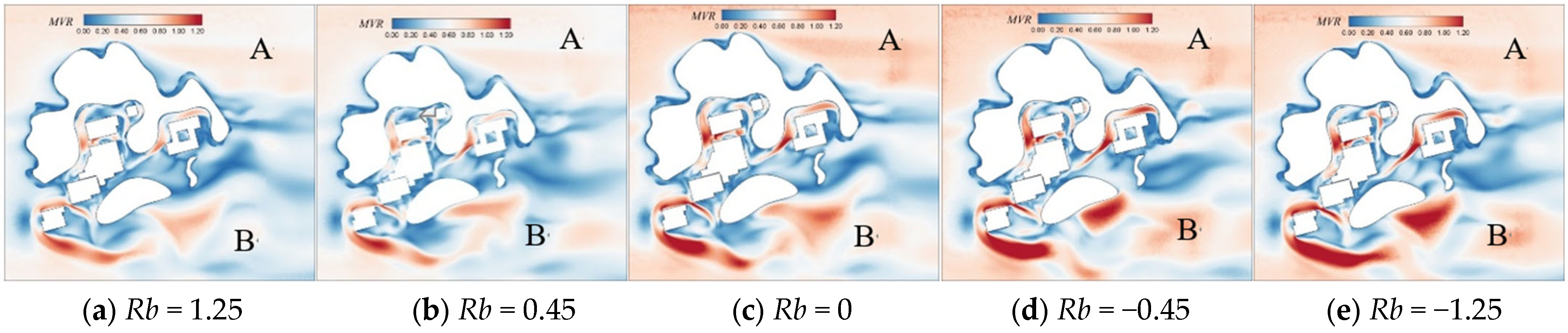
To determine the influence of different thermal conditions on pollutant dispersion in the simulation, five Rb values (Rb = −1.25, −0.45, 0, 0.45, and 1.25) were used to analyse the flow field in the case study. Figure 16 shows the PLW MVR contours according to different thermal conditions, in which it can be observed that the dimensionless flow field distribution maintained the same trend regardless of the thermal condition. However, in open areas, such as locations A and B, the dimensionless wind speed increased under decreasingly stable thermal conditions: the maximum MVR was obtained when Rb = −1.25, and the minimum MVR was obtained when Rb = 1.25. This indicates that unstable thermal conditions (represented by negative Rb values) cause a higher wind speed near the ground, promoting the diffusion of pollutants, whereas stable thermal conditions (represented by positive Rb values) have the opposite trend.
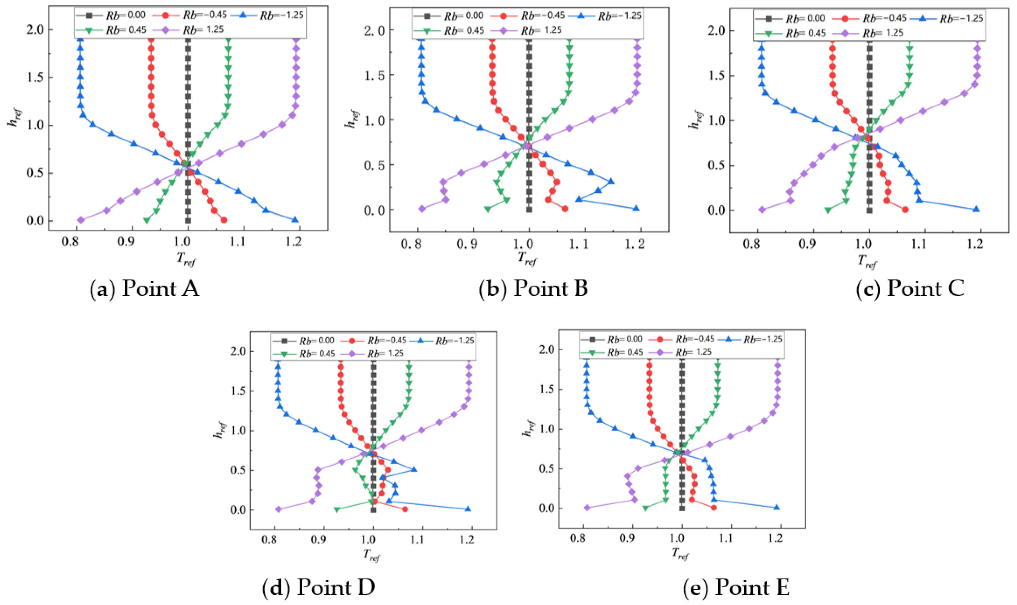
To further explore the mechanism by which the thermal condition affects the pollutant concentration distribution, the temperature profiles of the same five points were analysed along the height direction, as shown in Figure 17, in which Tref is the absolute temperature. It can be seen in the figure that point A was not disturbed by the surface, and the temperature was basically the same as the inlet flow. Points B, C, D, and E were leeward of the building model, where the temperature distribution exhibited an obvious change below 0.6href. The temperature below 0.6href was completely different from the inlet temperature, especially at points D and E, following inconsistent trends. Thus, the change in pollutant concentration exhibited no obvious regularity according to the thermal condition.
4.4.3. Distribution of Pollutant Concentration
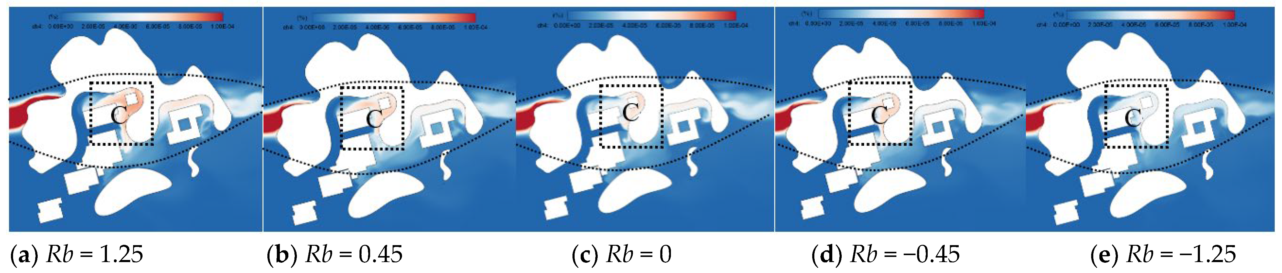
Figure 18 shows the pedestrian-height pollutant concentration distribution around the hospital according to the thermal condition. It can be observed that the flow field was influenced by a complex terrain, and the diffusion of pollutants around the hospital was contained within an area that was about 260 m long, or about four times the characteristic length of the building, as indicated by the dotted line. In region C, located behind building 3, the flow field was blocked by the surrounding mountainous terrain, allowing pollutants to readily accumulate in the area. Furthermore, Figure 18 indicates that the pollutant concentration was significantly higher under stable thermal conditions than under unstable thermal conditions.
Figure 19 shows the pollutant concentration distribution along the y = 0 sectional plane according to the thermal condition, in which it can be observed that the pollutant concentration decreased with increasing longitudinal distance. In Figure 19, the mountainous area and buildings are both in region D, where the flow field is highly disturbed by this complex terrain. In contrast, region E is a relatively flat area, where the flow field is relatively stable. The figure indicates that the concentration of pollutants in region D first increased and then decreased with increasingly unstable thermal conditions, representing a notable deviation from the conventional atmospheric stability theory. In region E, the pollutant concentration decreased consistently with increasingly unstable thermal conditions. Therefore, in an area with significant surface roughness, the concentration of pollutants will be affected considerably by the disturbance of the surface wind field, and the effect of the thermal stability of the atmosphere on the pollutant diffusion is relatively small. However, in relatively flat regions, the thermal stability of the atmosphere plays a significant role in pollutant diffusion.
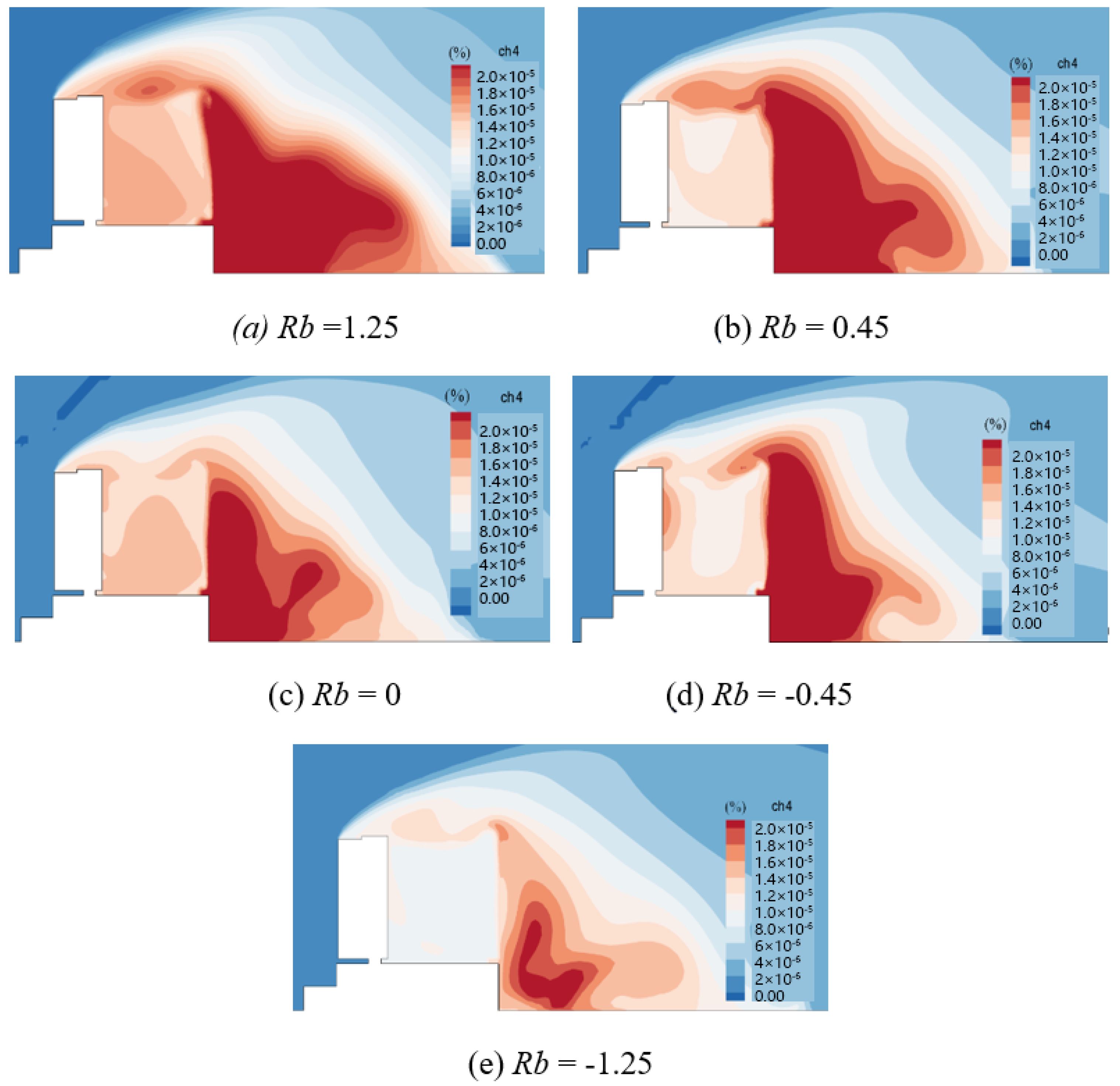
A local quantitative analysis of the pollutant concentration around building 3 was then conducted, with the results being shown in Figure 20. It can be observed that the blocking effect of the building prevents the air inside the yard from flowing readily, and the pollutant diffusion exhibits no apparent law according to the thermal condition. However, in the relatively open location at the tail of the building, the pollutant concentration is monotonically related to the thermal condition. The concentration of pollutants reached its maximum under stable thermal conditions, when Rb = 1.25. Such stable conditions generally occur in the morning or evening during winter, at which time special attention should be paid to the hazards posed by pollutants.
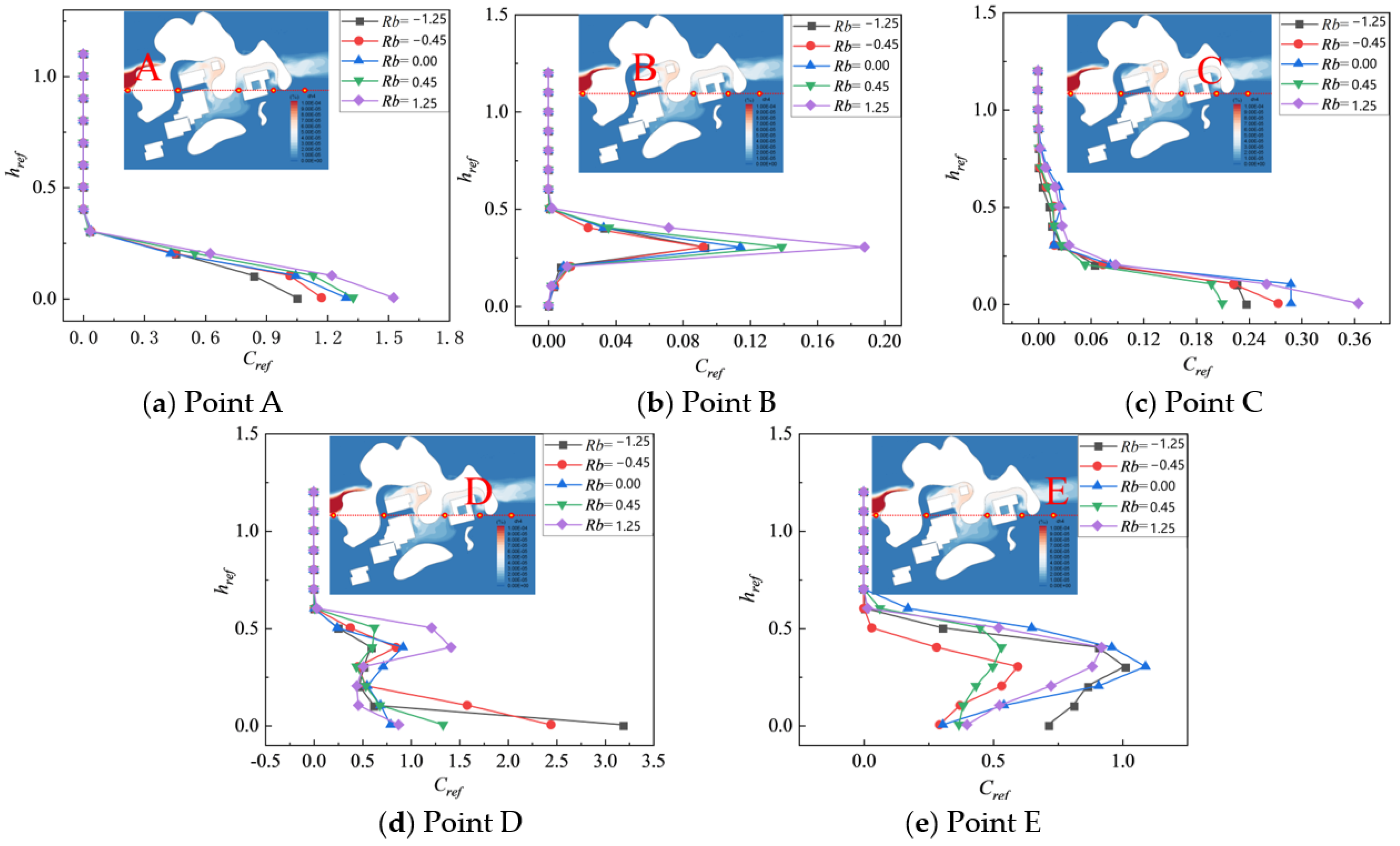
To quantitatively evaluate the pollutant concentration in different regions, measurements were collected at different heights at five points, labelled A, B, C, D, and E, along the y = 0 sectional plane of the simulation model, as shown in Figure 21. Point A was selected on the left of the mountain, where the flow field was not disturbed by surface roughness; the concentration of pollutants mainly remained below 0.25href, and the pollutant concentration increased with increasingly unstable thermal conditions. Point B was selected in the ventilation corridor; the pollutant concentration was relatively low, with its maximum value occurring near 0.3href and increasing consistently with increasingly unstable thermal conditions. Points C, D, and E were selected downwind of the hospital, where the wind field was significantly influenced by the terrain; as a result, the pollutant concentrations exhibited no obvious regularity, but were considerably affected by the thermal stability of the atmosphere. In areas with significant surface roughness, the pollutant concentration was affected by the interaction between the thermal conditions and complex surface turbulence, so the diffusion mechanism was more complex.
5. Conclusions
This study conducted experimental and numerical analyses of the outdoor wind environment around an infectious disease hospital in Changsha, considering the effects of thermal conditions. The wind field and pollutant concentration distributions were obtained according to the thermal stability of the atmosphere, and the following conclusions were obtained accordingly:
- (1)
- The results of the wind tunnel tests showed that the thermal conditions had little effect on the longitudinal component of the wind profile in the range of Rb = 0 to 0.38. The absolute value of the methane tracer gas concentration depended on the local wind speed. The maximum methane concentration occurred near the ground and decreased with increasing height. The influence of the thermal conditions on the methane tracer gas concentration mainly occurred below 60% of the building height; the pollutant concentration tended to be stable at heights that were greater than the building height.
- (2)
- The wind tunnel tests were able to capture the influence of the building layout on pollutant concentrations around the case study hospital, indicating that the coupling effects between the building shape, local wind speed, and direction should be considered in hospital planning. An orientation in which the building ventilation features were aligned with the dominant wind direction was most conducive to the reduction in pollutant concentrations.
- (3)
- Detailed flow field distributions around the case study hospital under different thermal conditions were obtained using verified numerical simulations. The results indicated that the concentration of pollutants was mainly affected by the disturbance of the flow field in areas with large surface roughness, and the effect of the thermal stability of the atmosphere on pollutant diffusion was relatively small in the range of Rb = −1.25 to 1.25. In relatively flat regions, the thermal stability of the atmosphere played a significant role in pollutant diffusion.
Author Contributions
Writing—original draft, Y.Y.; Writing—review & editing, J.H.; Project administration, Y.T.; Data curation, K.W.; Validation, L.S. All authors have read and agreed to the published version of the manuscript.
Funding
Changsha University of Science and Technology Graduate Research Innovation Project (CSLGCX23027). 2023 Hubei Construction Science and Technology Programme Project.
Data Availability Statement
The data that support the findings of this study are available on request from the corresponding author, Lian Shen, upon reasonable request.
Conflicts of Interest
Authors Ying Yang and Yigao Tan were employed by the company China Construction Fifth Engineering Bureau Co., Ltd. The remaining authors declare that the research was conducted in the absence of any commercial or financial relationships that could be construed as a potential conflict of interest.
References
- Wang, H.Q.; Huang, C.H.; Di, L.; Zhao, F.Y.; Sun, H.B.; Wang, F.F.; Li, C.; Ye, M.Q. Fume transports in a high rise industrial welding hall with displacement ventilation system and individual ventilation units. Build. Environ. 2012, 52, 119–128. [Google Scholar] [CrossRef]
- Zheng, X.; Montazeri, H.; Blocken, B. Large-eddy simulation of pollutant dispersion in generic urban street canyons: Guidelines for domain size. J. Wind Eng. Ind. Aerodyn. 2021, 211, 104527. [Google Scholar] [CrossRef]
- Dwivedi, A.; Khire, M.V. Application of split window algorithm to study Urban Heat Island effect in Mumbai through land surface temperature approach. Sustain. Cities Soc. 2018, 41, 865–877. [Google Scholar] [CrossRef]
- Ho, C.K. Modeling airborne pathogen transport and transmission risks of SARS-CoV-2. Appl. Math. Model. 2021, 95, 297–319. [Google Scholar] [CrossRef] [PubMed]
- Baik, J.J.; Park, R.S.; Chun, H.Y.; Kim, J.J. A laboratory model of urban street canyon flows. J. Appl. Meteorol. 2000, 39, 1592–1600. [Google Scholar] [CrossRef]
- Kellnerova, R.; Kukacka, L.; Jurcakova, K.; Uruba, V.; Janour, Z. PIV measurement of turbulent flow within a street canyon: Detection of coherent motion. J. Wind Eng. Ind. Aerodyn. 2012, 104, 302–313. [Google Scholar] [CrossRef]
- Gromke, C.; Buccolieri, R.; Sabatino, S.D.; Ruck, B. Dispersion study in a street canyon with tree planting by means of wind tunnel and numerical investigationse evaluation of CFD data with experimental data. Atmos. Environ. 2008, 42, 8640–8650. [Google Scholar] [CrossRef]
- Ai, Z.T.; Mak, C.M. CFD simulation of flow and dispersion around an isolated building: Effect of inhomogeneous ABL and near-wall treatment. Atmos. Environ. 2013, 77, 568–578. [Google Scholar] [CrossRef]
- Ai, Z.T.; Mak, C.M.; Niu, J.L. Numerical investigation of wind-induced airflow and interunit dispersion characteristics in multistory residential buildings. Indoor Air 2013, 23, 417–429. [Google Scholar] [CrossRef] [PubMed]
- Lateb, M.; Masson, C.; Stathopoulos, T.; Bedard, C. Comparison of various types of k-ε models for pollutant emissions around a two-building configuration. J. Wind Eng. Ind. Aerodyn. 2013, 115, 9–21. [Google Scholar] [CrossRef]
- Cheng, Y.; Lee, S.C.; Gao, Y.; Cui, L.; Deng, W.; Cao, J.; Sun, J. Real-time measurements of PM2.5, PM10-2.5, and BC in an urban street canyon. Particuology 2015, 20, 134–140. [Google Scholar] [CrossRef]
- Liu, Y.S.; Cui, G.X.; Wang, Z.S.; Zhang, Z.S. Large eddy simulation of wind field and pollutant dispersion in downtown Macao. Atmos. Environ. 2011, 45, 2849–2859. [Google Scholar] [CrossRef]
- Nardecchia, F.; Gugliermetti, F.; Bisegna, F. How temperature affects the airflow around a single-block isolated building. Energy Build. 2016, 118, 142–151. [Google Scholar] [CrossRef]
- Xie, Z.; Castro, I.P. LES and RANS for turbulent flow over arrays of Wall-Mounted obstacles. Flow Turbul. Combust. 2006, 76, 291–312. [Google Scholar] [CrossRef]
- Tominaga, Y.; Mochida, A.; Yoshie, R.; Kataoka, H.; Nozu, T.; Yoshikawa, M.; Shirasawa, T. AIJ guidelines for practical applications of CFD to pedestrian wind environment around buildings. J. Wind Eng. Ind. Aerodyn. 2008, 96, 1749–1761. [Google Scholar] [CrossRef]
- Blocken, B. Computational Fluid Dynamics for urban physics: Importance, scales, possibilities, limitations and ten tips and tricks towards accurate and reliable simulations. Build. Environ. 2015, 91, 219–245. [Google Scholar] [CrossRef]
- Ouyang, Y.; Jiang, W.M.; Hu, F.; Miao, S.G.; Zhang, N. Experimental study in wind yunnel in the field of air flows and pollutant dispersion in the urban sub-domain. J. Nanjing Univ. Nat. Sci. 2003, 6, 770–780. [Google Scholar]
- Hajra, B.; Stathopoulos, T. A Wind Tunnel Study of the Effect of Downstream Buildings on Near-field Pollutant Dispersion. Build. Environ. 2012, 52, 19–31. [Google Scholar] [CrossRef]
- Gousseau, P.; Blocken, B.; Stathopoulos, T.; Heijst, G.J.F. CFD simulation of near-field pollutant dispersion on a high-resolution grid: A case study by LES and RANS for a building group in downtown Montreal. Atmos. Environ. 2011, 45, 428–438. [Google Scholar] [CrossRef]
- Liu, X.P.; Niu, J.L.; Kwok, K.C.S.; Wang, J.H.; Li, B.Z. Investigation of indoor air pollutant dispersion and cross-contamination around a typical high-rise residential building: Wind tunnel tests. Build. Environ. 2010, 45, 1769–1778. [Google Scholar] [CrossRef]
- Huang, Y.D.; Wang, S.S.; Jin, X.; Sun, Y.N.; Jin, M.X. A comparative study of various turbulence models for simulating pollutant dispersion within an urban street canyon. J. Hydrodyn. 2008, 23, 189–195. [Google Scholar]
- Zhang, Y.; Kwok, K.C.S.; Liu, X.R.; Niu, J.L. Characteristics of air pollutant dispersion around a high-rise building. Environ. Pollut. 2015, 204, 280–288. [Google Scholar] [CrossRef] [PubMed]
- Shi, R.; Cui, G.; Wang, Z. Large eddy numerical simulation of urban residential area, air flow and traffic pollution. Prog. Nat. Sci. 2009, 19, 212–221. [Google Scholar]
- Health, Welfare & Food Bureau, 28 May 2003. Government of the Hong Kong Special Administrative Region. SARS Bulletin; 2012. Available online: http://www.info.gov.hk/info/sars/bulletin/bulletin0528e.pdf (accessed on 20 September 2008).
- Niu, J.; Tung, T.C.W. On-site quantification of re-entry ratio of ventilation exhausts in multi-family residential buildings and implications. Indoor Air 2008, 18, 12–26. [Google Scholar] [CrossRef] [PubMed]
- Gao, N.P.; Niu, J.L.; Perino, M.; Heiselberg, P. The airborne transmission of infection between flats in high-rise residential buildings: Tracer gas simulation. Build. Environ. 2008, 43, 1805–1817. [Google Scholar] [CrossRef] [PubMed]
- Wang, J.H.; Niu, J.L.; Liu, X.P.; Yu, C.W.F. Assessment of pollutant dispersion in the re-entrance space of a high-rise residential building, Using wind tunnel simulations. Indoor Built Environ. 2010, 19, 638–647. [Google Scholar] [CrossRef]
- Chao, L.A.; Ro, B.; Hk, B.; Ts, C.; Ma, C. Wind tunnel experiment on high-buoyancy gas dispersion around isolated cubic building. J. Wind. Eng. Ind. Aerodyn. 2020, 202, 104–226. [Google Scholar]
- Mestayer, A.P.G. Pollutant dispersion and thermal effects in urban street canyons. Atmos. Environ. 1996, 30, 2659–2677. [Google Scholar]
- Baik, J.J.; Kim, J.J. A numerical study of flow and pollutant dispersion characteristics in urban street canyons. J. Appl. Meteorol. 1999, 38, 1576–1589. [Google Scholar] [CrossRef]
- Xie, X.; Liu, C.H.; Leung, D.Y.C.; Leung, M.K.H. Characteristics of air exchange in a street canyon with ground heating. Atmos. Environ. 2006, 40, 6396–6409. [Google Scholar] [CrossRef]
- Li, X.X.; Liu, C.H.; Leung, D.Y.C. Large-Eddy simulation of flow and pollutant dispersion in High-Aspect-Ratio urban street canyons with wall model. Bound.-Layer Meteorol. 2008, 129, 249–268. [Google Scholar] [CrossRef]
- Li, X.X.; Britter, R.E.; Koh, T.Y.; Norford, L.K.; Liu, C.H.; Entekhabi, D.; Leung, D.Y.C. Large–Eddy simulation of flow and pollutant transport in urban street canyons with ground heating. Bound.-Layer Meteorol. 2010, 137, 187–204. [Google Scholar] [CrossRef]
- Li, X.X.; Britter, R.E.; Norford, L.K.; Koh, T.Y.; Entekhabi, D. Flow and pollutant transport in urban street canyons of different aspect ratios with ground heating: Large–Eddy simulation. Bound.-Layer Meteorol. 2012, 142, 289–304. [Google Scholar] [CrossRef]
- Dallman, A.; Magnusson, S.; Britter, R.; Norford, L.; Entekhabi, D.; Fernando, H.J.S. Conditions for thermal circulation in urban street canyons. Build. Environ. 2014, 80, 184–191. [Google Scholar] [CrossRef]
- Hang, C.; Nadeau, D.F.; Jensen, D.D.; Hoch, S.W.; Pardyjak, E.R. Playa soil moisture and evaporation dynamics during the MATERHORN field program. Bound.-Layer Meteorol. 2016, 159, 521–538. [Google Scholar] [CrossRef]
- Cui, P.Y.; Li, Z.; Tao, W.Q. Wind-tunnel measurements for thermal effects on the air flow and pollutant dispersion through different scale urban areas. Build. Environ. 2016, 97, 137–151. [Google Scholar] [CrossRef]
- Cheng, W.C.; Liu, C.H. Large-eddy simulation of turbulent transports in urban street canyons in different thermal stabilities. J. Wind Eng. Ind. Aerodyn. 2011, 99, 434–442. [Google Scholar] [CrossRef]
- Xie, Z.T.; Hayden, P.; Wood, C.R. Large–eddy simulation of approaching–flow stratification on dispersion over arrays of buildings. Atmos. Environ. 2013, 71, 64–74. [Google Scholar] [CrossRef]
- Boppana, V.B.L.; Xie, Z.T.; Castro, I.P. Thermal stratification effects on flow over a generic urban canopy. Bound. Layer Meteorol. 2014, 153, 141–162. [Google Scholar] [CrossRef]
- Li, X.X.; Britter, R.E.; Norford, L.K. Transport processes in and above two-dimensional urban street canyons under different stratification conditions: Results from numerical simulation. Environ. Fluid Mech. 2015, 15, 399–417. [Google Scholar] [CrossRef]
- Tomas, J.M.; Pourquie, M.J.B.M.; Jonker, H.J.J. The influence of an obstacle on flow and pollutant dispersion in neutral and stable boundary layers. Atmos. Environ. 2015, 113, 236–246. [Google Scholar] [CrossRef]
- Irwin, H. A simple omnidirectional sensor for wind-tunnel studies of pedestrian-level winds. J. Wind Eng. Ind. Aerodyn. 1981, 7, 219–239. [Google Scholar] [CrossRef]
- Wu, H.; Stathopoulos, T. Further experiments on Irwin’s surface wind sensor. J. Wind Eng. Ind. Aerodyn. 1994, 53, 441–452. [Google Scholar] [CrossRef]
- Monteiro, J.P.; Viegas, D.X. On the use of Irwin and Preston wall shear stress probes in turbulent incompressible flows with pressure gradients. J. Wind Eng. Ind. Aerodyn. 1996, 64, 15–29. [Google Scholar] [CrossRef]
- Fluent. Fluent 18.0 Documentation [R]; Fluent Inc.: New York, NY, USA, 2014. [Google Scholar]
- Ferziger, J.H.; Peric, M. Computational Methods for Fluid Dynamics; Springer: Berlin/Heidelberg, Germany, 2002; p. 50. [Google Scholar]
Figure 1.
Wind tunnel.

Figure 2.
Irwin sensors.

Figure 3.
Heating device.

Figure 4.
Pollutant concentration test devices.

Figure 5.
Schematic of pollutant dispersion wind tunnel test. NOTE: 1. Wind tunnel; 2. wedge; 3. roughness element; 4. air pump; 5. methane supply tank; 6. flowmeter; 7. spiral tube; 8. magnetic bead glass bottle; 9. pollutant emitter; 10. building model; 11. fixed frame; 12. collecting rake; 13. monitoring tube; 14. delivery pump; 15. collecting bags; 16. chromatographic analyser; and 17. computer.

Figure 6.
Wind tunnel model and test setup.

Figure 7.
Comparison of PLW MVR values according to thermal condition.

Figure 8.
Wind profiles at point 16 according to thermal condition.

Figure 9.
Methane concentration profiles for different Rb numbers.

Figure 10.
Four cases with different building orientations.

Figure 11.
Methane tracer gas concentration at pedestrian level according to thermal condition (points 2–4 in the south-western part of the model, points 12–14 in the eastern of the model).
Figure 11.
Methane tracer gas concentration at pedestrian level according to thermal condition (points 2–4 in the south-western part of the model, points 12–14 in the eastern of the model).

Figure 12.
Methane tracer gas concentration profiles at point 17 according to building orientation.

Figure 13.
Calculation domain and meshes.


Figure 14.
Comparison of the test’s obtained and simulated wind profiles.

Figure 15.
Comparison of the test’s obtained and simulated methane tracer gas concentration profiles.
Figure 15.
Comparison of the test’s obtained and simulated methane tracer gas concentration profiles.

Figure 16.
Pedestrian-height MVR contours according to different thermal conditions.

Figure 17.
Temperature distributions along the height direction according to the thermal condition.

Figure 18.
Pedestrian-height pollutant concentration contours according to thermal condition.

Figure 19.
Pollutant concentration contours at plane y = 0 according to thermal condition.

Figure 20.
Pollutant concentrations behind building 3 according to thermal condition.

Figure 21.
Pollutant concentration profile under different thermal conditions.


Table 1.
Wind tunnel test cases.
| Factor | Cases | Description | Rb | Building Orientation |
|---|---|---|---|---|
| Thermal effect | 1 | Average wind speed: 1.2 m/s | 0 | 0° |
| 2 | Average wind speed: 1.2 m/s | −0.17 | 0° | |
| 3 | Average wind speed: 1.2 m/s | −0.28 | 0° | |
| 4 | Average wind speed: 1.2 m/s | −0.38 | 0° | |
| Building orientation | 5 | Average wind speed: 1.2 m/s | 0 | 0° |
| 6 | Average wind speed: 1.2 m/s | 0 | 45° | |
| 7 | Average wind speed: 1.2 m/s | 0 | 90° | |
| 8 | Average wind speed: 1.2 m/s | 0 | 135° |
Table 2.
Boundary conditions.
| Name | Boundary | Conditions |
|---|---|---|
| Inlet | Velocity inlet | 1.2 m/s |
| Outlet | Outflow | |
| Top surface | Free slip wall | |
| Bottom surface | No slip wall | u = 0, v = 0, w = 0, ∂p/∂n = 0 |
| Side surface | Symmetric boundary | |
| Building and mountain surface | No slip wall | u = 0, v = 0, w = 0, ∂p/∂n = 0 |
Disclaimer/Publisher’s Note: The statements, opinions and data contained in all publications are solely those of the individual author(s) and contributor(s) and not of MDPI and/or the editor(s). MDPI and/or the editor(s) disclaim responsibility for any injury to people or property resulting from any ideas, methods, instructions or products referred to in the content. |
© 2024 by the authors. Licensee MDPI, Basel, Switzerland. This article is an open access article distributed under the terms and conditions of the Creative Commons Attribution (CC BY) license (https://creativecommons.org/licenses/by/4.0/).
Share and Cite
MDPI and ACS Style
Yang, Y.; Hu, J.; Tan, Y.; Wang, K.; Shen, L. Pollutant Diffusion in an Infectious Disease Hospital with Different Thermal Conditions. Buildings 2024, 14, 1185. https://doi.org/10.3390/buildings14041185
AMA Style
Yang Y, Hu J, Tan Y, Wang K, Shen L. Pollutant Diffusion in an Infectious Disease Hospital with Different Thermal Conditions. Buildings. 2024; 14(4):1185. https://doi.org/10.3390/buildings14041185
Chicago/Turabian StyleYang, Ying, Jiayi Hu, Yigao Tan, Kuo Wang, and Lian Shen. 2024. "Pollutant Diffusion in an Infectious Disease Hospital with Different Thermal Conditions" Buildings 14, no. 4: 1185. https://doi.org/10.3390/buildings14041185
Note that from the first issue of 2016, this journal uses article numbers instead of page numbers. See further details here.