Article

Deep Reinforcement Learning for Flow Control Exploits Different Physics for Increasing Reynolds Number Regimes

1
CMT—Motores Térmicos, Universitat Politècnica de València, 46022 Valencia, Spain
2
Barcelona Super Computing Center—Centro Nacional de Supercomputación (BSC-CNS), 08034 Barcelona, Spain
3
FLOW, Engineering Mechanics, KTH Royal Institute of Technology, 114 28 Stockholm, Sweden
4
Norwegian Meteorological Institute, 0313 Oslo, Norway
*
Author to whom correspondence should be addressed.
Actuators 2022, 11(12), 359; https://doi.org/10.3390/act11120359
Submission received: 31 October 2022 / Revised: 28 November 2022 / Accepted: 29 November 2022 / Published: 2 December 2022
(This article belongs to the Special Issue Active Flow Control: Recent Advances in Fundamentals and Applications)

Abstract

:
The increase in emissions associated with aviation requires deeper research into novel sensing and flow-control strategies to obtain improved aerodynamic performances. In this context, data-driven methods are suitable for exploring new approaches to control the flow and develop more efficient strategies. Deep artificial neural networks (ANNs) used together with reinforcement learning, i.e., deep reinforcement learning (DRL), are receiving more attention due to their capabilities of controlling complex problems in multiple areas. In particular, these techniques have been recently used to solve problems related to flow control. In this work, an ANN trained through a DRL agent, coupled with the numerical solver Alya, is used to perform active flow control. The Tensorforce library was used to apply DRL to the simulated flow. Two-dimensional simulations of the flow around a cylinder were conducted and an active control based on two jets located on the walls of the cylinder was considered. By gathering information from the flow surrounding the cylinder, the ANN agent is able to learn through proximal policy optimization (PPO) effective control strategies for the jets, leading to a significant drag reduction. Furthermore, the agent needs to account for the coupled effects of the friction- and pressure-drag components, as well as the interaction between the two boundary layers on both sides of the cylinder and the wake. In the present work, a Reynolds number range beyond those previously considered was studied and compared with results obtained using classical flow-control methods. Significantly different forms of nature in the control strategies were identified by the DRL as the Reynolds number R e increased. On the one hand, for R e 1000 , the classical control strategy based on an opposition control relative to the wake oscillation was obtained. On the other hand, for R e = 2000 , the new strategy consisted of energization of the boundary layers and the separation area, which modulated the flow separation and reduced the drag in a fashion similar to that of the drag crisis, through a high-frequency actuation. A cross-application of agents was performed for a flow at R e = 2000 , obtaining similar results in terms of the drag reduction with the agents trained at R e = 1000 and 2000. The fact that two different strategies yielded the same performance made us question whether this Reynolds number regime ( R e = 2000 ) belongs to a transition towards a nature-different flow, which would only admits a high-frequency actuation strategy to obtain the drag reduction. At the same time, this finding allows for the application of ANNs trained at lower Reynolds numbers, but are comparable in nature, saving computational resources.

1. Introduction

In transport applications (especially, in aeronautics), drag reduction is directly related to a decrease in fuel use, which translates into reducing pollution and greenhouse-gas emissions [1]. In the past decades, several techniques have been developed and used to reduce drag, both passively (Bechert and Bartenwerfer [2]) and actively (Gad-el Hak [3]). Passive methods typically rely on fixed geometric changes without using actuators. An example of this technology would be the widespread use of winglets in aircraft. Inspired by bird wings, winglets consist of small wing extensions at the wing tip with an angle relative to the wing-span direction. Using winglets, lift-induced drag is decreased by reducing the size and formation of vortices at the wing tip [4], incurring (hopefully) small increases in the structural weight and parasitic drag. Regarding active methods, diverse techniques are used to reduce aircraft drag and associated emissions. In the work of Tiseira et al. [5] and Serrano et al. [6,7], the use of distributed electric propulsion is combined with boundary-layer ingestion, setting small propellers along the wing near the trailing edge. Thanks to both technologies, it is possible to increase the aerodynamic efficiency of small aircraft or unmanned air vehicles (UAVs). In the same way, the location and use of both jet pumps in wings and synthetic jets are studied to reduce the drag of different aerodynamic bodies. An example of blowing and suction used to control turbulent boundary layers is provided by Kametani and Fukagata [8], and a number of studies have shown the feasibility of this approach in turbulent wings [9,10,11,12].
Additional examples can be found in the work of Voevodin et al. [13] and Yousefi and Saleh [14], where the placement of the suction and ejection in wing airfoils is studied to reduce aerodynamic drag or achieve efficient control of the flow around the wing in specific flight-operating conditions. In the same way, the use of synthetic jets has been studied to achieve this same objective, as displayed in the work of Cui et al. [15] on an Ahmed body, or the investigation of Park et al. [16] using an array of synthetic jets applied to a car. A comprehensive review of active flow control in a turbulent flow is provided by Choi et al. [17].
Active-control methods rely on complicated control strategies due to their variable behaviors and dependencies. As shown by Muddada and Patnaik [18], even the control of simple actuators to reduce the drag of a cylinder immersed in a low Reynolds number flow can be complicated due to the interaction between boundary layers, separating shear layers and wake. In this case, by correctly developing a control algorithm, the drag is reduced by about 53%, leaving ample room for improvement in the case of achieving better control. However, thanks to the application of artificial neural networks (ANNs) and deep reinforcement learning (DRL), it is possible to develop functional control strategies at an affordable computational cost in similar problems, as shown by the work by Rabault et al. [19]. An ANN is a non-parametric tool formed by layers of connected processing nodes or neurons and it can be trained to solve complex problems [20,21]. The ANN training can take place through different types of learning, where DRL is one of the fastest-growing in solving a wide range of cases [22,23], including flow control in complex geometries [24,25].
DRL is based on maximizing a reward by means of an agent interacting with the environment through actions, based on partial observations of the environment. Note that the combination of DRL and ANN was successfully carried out to solve active flow control in the work of Rabault et al. [19]. A proximal policy optimization (PPO) is used to obtain the control policy of two synthetic jets on a two-dimensional cylinder in a low Reynolds number flow. PPO parameterizes a policy function using an ANN with a set of neuron weights given an observation state. The ANN then produces a set of moments that describe a distribution function from which actions are sampled. It is possible to obtain an expression for the estimation of the gradient of the reward as a function of the neuron weights. Additionally, the PPO uses a critic network that estimates the new reward function, which is helpful with stochastic data. Moreover, there is a limit to the maximum update at every training step, preventing rare events from producing large rewards [26]. It was shown that DRL was feasible and enabled finding a control strategy, such that the cylinder drag was reduced by 8%. Rabault and Kuhnle [27] developed a framework to parallelize environments, enabling speeding up computation and learning, thus reaching a better solution faster. Additionally, Tang et al. [28] validated the DRL approach in a more complex problem using four jets on the cylinder and extending the Reynolds number range. The results of Rabault et al. in [19,27] have been utilized in a multitude of studies in recent years. For example, the works of Tokarev et al. [29] and Xu et al. [30], where oscillatory rotary controls were applied to the cylinder; the study of linear stability and low sensitivity that allows a better understanding of DRL by Li and Zhang [31], or the effort of Ren et al. [32] where the same DRL approach is used with a solver that allows calculations at higher Reynolds numbers, with the additional problem of controlling the increase in turbulence around the cylinder. Applications to square cylinders, which are relevant to civil engineering, have also been presented recently [33], as well as using traditional modal analysis methods for defining effective reward functions [34]. Regarding these works, there is room for improvement through the application of high-performance computing (HPC), enabling conducting faster calculations at higher Reynolds numbers not previously calculated.
The main objective of this work is, indeed, to demonstrate the capabilities of the HPC resources available today to perform aerodynamic optimization with DRL-based control at much higher Reynolds numbers than the ones already studied in the literature. This project proposes the use of the numerical code Alya, developed in the Barcelona Supercomputer Center (BSC-CNS) [35], employing the HPC MareNostrum IV cluster. Alya is a tier-0 massively parallel code and is designed to solve discretized partial differential equations using finite elements. This code has been successfully used in different problems of fluid mechanics, including simulations of turbulent flows [36,37].
In the present work, the methodology is first detailed in Section 2, dedicated to the numerical setup and the application of the DRL and the ANN. The results are then summarized and discussed in Section 3, which starts with the validation of the Alya solver in the combination of an HPC cluster to solve the DRL problem in the cylinder. Then, the results derived from the increase in the Reynolds number, which exceed the conditions reported in the literature, are shown. Finally, the main conclusions are collected in Section 4.

2. Methods

This section is divided into two parts: (1) the problem description and the domain setup along the methodology (regarding the numerical simulations) and (2) the framework, including the DRL algorithm.

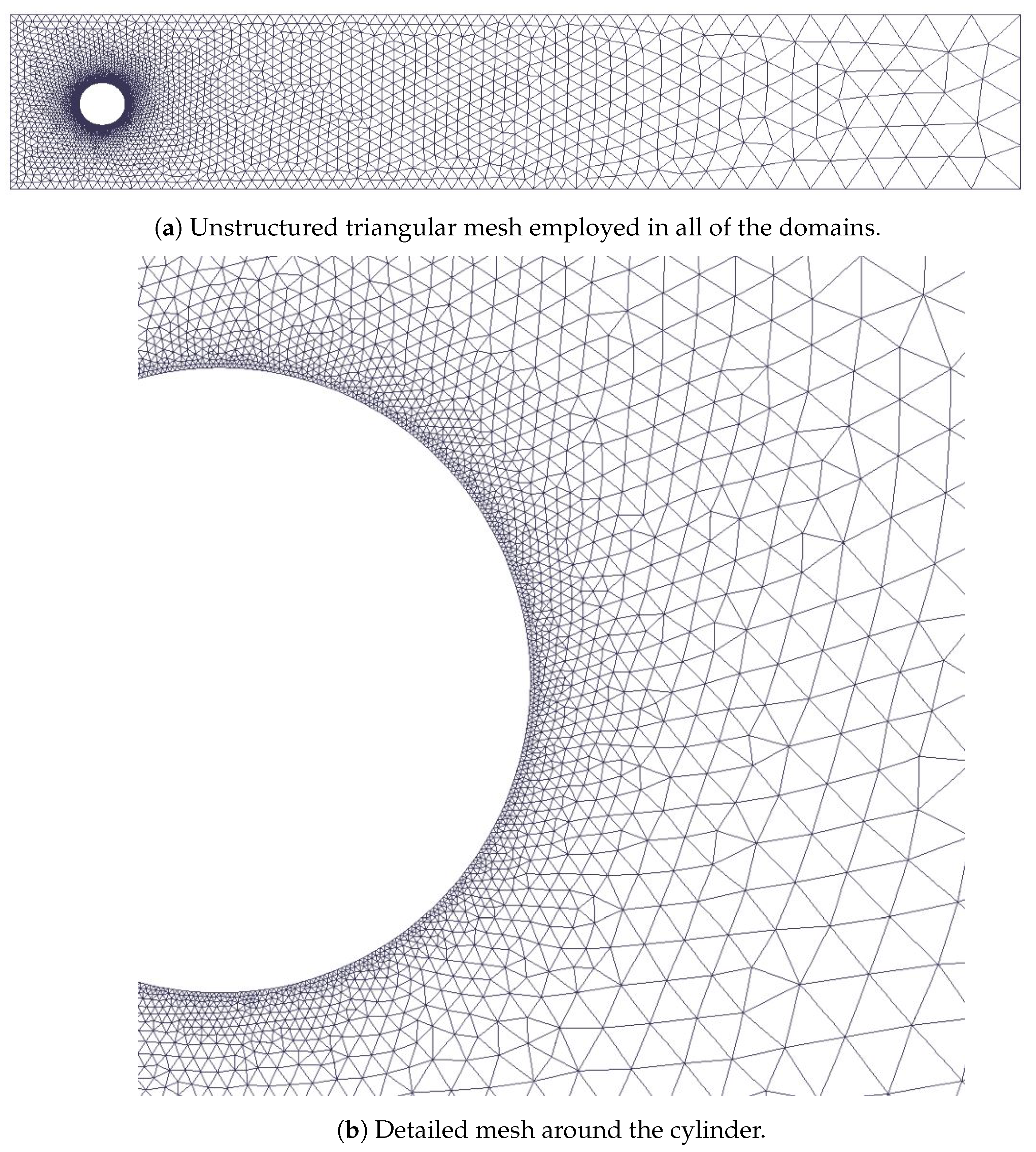
2.1. Problem Configuration and Numerical Setup
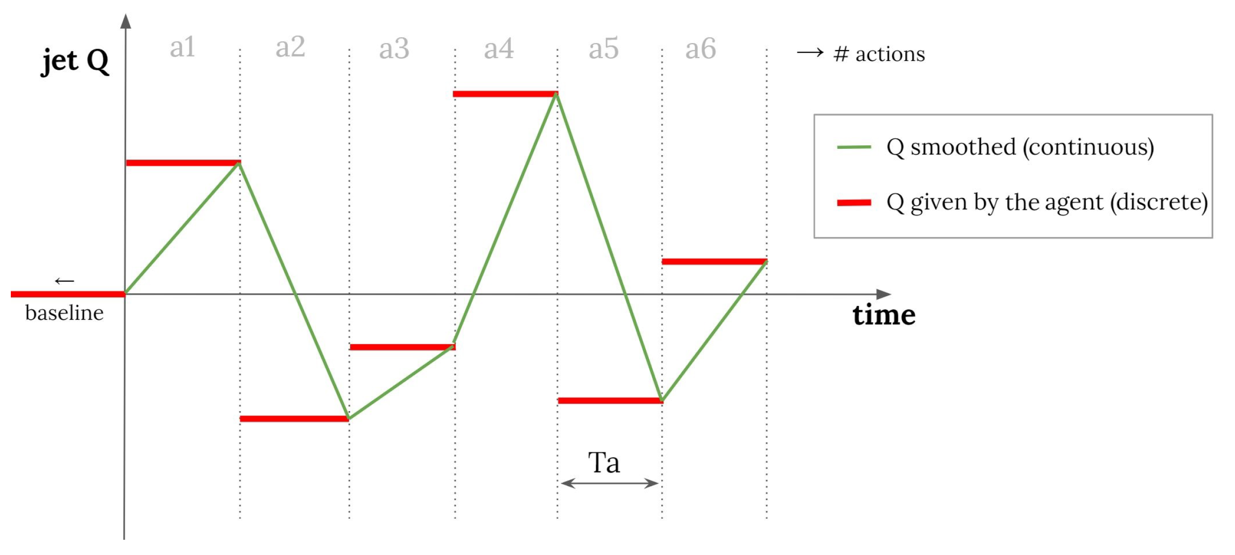
The domain simulation is two-dimensional (2D) and consists of a cylinder immersed in a flat rectangular channel without any curvature, in the same configuration as that described in the work by Rabault et al. [19]. The domain is normalized using a cylinder with diameter D as the reference length scale. The channel has a dimension of L = 22 in length, aligned with the main flow direction, and a height equal to H = 4.1 . The origin of the coordinate system is set on the left-bottom corner of the channel, and the center of the cylinder displaced towards the bottom by 0.05 D units, to develop the vortex-shedding behind it. A schematic representation of the domain is depicted in Figure 1. Aligned with the vertical axis and symmetrically on the cylinder wall, one at the top and one at the bottom, there are two synthetic jets with total openings of ω = 10 each. These positions of the jets were chosen so their actuations were normal to the flow and drag reduction came from effective actuations rather than the injection of momentum.
Regarding the boundary conditions of the problem, an inlet parabolic velocity condition was imposed and expressed as in Equation (1):
U in y = U max [ 1 2 y H / 2 H 2 ] ,
where [ U in ( y ) , V in ( y ) = 0 ] is the velocity vector and U max is the maximum velocity reached at the middle of the channel, which is equal to 1.5 times the mean velocity U ¯ , defined as shown in Equation (2):
U ¯ = 1 H 0 H U in ( y ) d y = 2 3 U max .
A value of U max = 1.5 is used so that the scaling velocity of the problem is U ¯ = 1 . A no-slip condition is imposed on the cylinder solid wall, while a smooth-wall condition is imposed on the channel walls. The right boundary of the channel is set as a free outlet with zero velocity gradient and constant pressure. The jet velocity ( v i ) is a function of both the set jet angle ( θ ) and the mass flow rate (Q) determined by the ANN, as described in Equation (3):
v i = Q π 2 ω R 2 cos [ π ω ( θ θ 0 ) ] ,
where θ 0 corresponds to the angle where the jet is centered and R is the cylinder radius. The scaling factor π / ( 2 ω R 2 ) is used so that the integration of the jet velocity over the jet width gives the desired mass flow rate Q. More details about the intensity parameters are provided in Section 2.2.
The Reynolds number R e = U ¯ D / ν of the simulation is varied between 100, 1000 and 2000, where ν is the fluid kinematic viscosity. For the mesh, an unstructured mesh of triangular elements with refinement near the cylinder wall and the jets was used, as shown in Figure 2. The number of elements changes with the Reynolds number as expressed in Table 1.
Alya is used to simulate the flow. This solver assumes that the flow is viscous and incompressible, where the governing Navier–Stokes equations can be written for a domain Ω as in Equation (5):
t u + ( u · ) u · ( 2 ν ϵ ) + p = f in Ω ( t 0 , t f ) ,
· u = 0 in Ω ( t 0 , t f ) ,
where ϵ is a function of the velocity u , which defines the velocity strain-rate tensor ( ϵ = 1 / 2 ( u + T u ) ) and f is the external body force. In Equation (4), the convective form of the nonlinear term, C nonc ( u ) = ( u · ) u , is expressed as a term conserving energy, momentum and angular momentum [38,39]. This form is known as EMAC (energy-, momentum-, and angular-momentum-conserving equation), and its expression appears in Equation (6). The EMAC form (Equation (6)) adds to the equation the conservation of energy as well as linear and angular momentum at the discrete level:
C emac = 2 u · ϵ + ( · u ) u 1 2 | u | 2 .
The spatial discretization of the Navier-Stokes equations is performed by means of the finite-element method (FEM). Meanwhile, the time discretization uses a semi-implicit Runge–Kutta scheme of second order for the convective term, and a Crank–Nicolson scheme for the diffusive term [40]. In the time integration, Alya uses an eigenvalue time-step estimation as described by Trias and Lehmkuhl [41]. The complete formulation of the flow solver is described in the work by Lehmkuhl et al. [37].
At each time step, the numerical solution is obtained, and the drag F D and lift F L forces are integrated over the cylinder surface S as follows (Equation (7)):
F = ( ς · n ) · e j d S ,
where ς is the Cauchy stress tensor, n is the unit vector normal to the cylinder and e j is a unit vector in the direction of the main flow velocity when calculating the drag and a vector perpendicular to the velocity of flow for the calculation of the lift force. The drag C D and lift C L coefficients are computed as described in Equations (8) and (9):
C D = 2 F D ρ U ¯ 2 D ,
C L = 2 F L ρ U ¯ 2 D .

2.2. DRL Setup

As discussed in the introduction, the DRL interacts with the domain through three channels. The first channel is the observation state (s), based on the extraction of pressure values at a series of predefined points along the domain. These points, known as witness points or probes, are located in the same positions as in Rabault et al. [19]. Moreover, 151 witness points were distributed around the cylinder and along the wake, as shown in Figure 3. The values of the pressure obtained at the witness points are normalized by a factor s norm so that the state values given to the agent are between 1 and 1, approximately. The values of s norm for each Reynolds number case are given in Table 1.
The second channel of interaction between the DRL and the numerical simulation is the action that is given by the control of the jets on the cylinder (a). The value of action a is directly related to the control value of the upper jet intensity Q 1 , while the bottom jet will do the opposite control to ensure a global zero mass flow rate between both jets, i.e., Q 2 = Q 1 . This is a more realistic control and helps to make the numerical scheme more stable as reflected by Rabault et al. [19]. During the training, the maximum value of | Q 1 | is limited to | Q 1 | < 0.06 Q ref 0.88 for the R e = 100 case, as in the work by Rabault et al. [19], to avoid unrealistically large actuations. Note that Q ref is the mass flow rate intercepting the cylinder, and it is calculated as in Equation (10):
Q ref = D / 2 D / 2 ρ U in ( y ) d y .
For higher Reynolds numbers, this clipping value of | Q 1 | is reduced to 0.04 . An observation should be made here about the energy consumption of the jets. If one reduces the drag, it would lead to a performance improvement. Nevertheless, the positive energy balance should be obtained when comparing the energy saved by reducing the drag compared with the energy used to actuate with the jets. However, one cannot determine the actual energy consumption of the jets in a numerical simulation, since this highly depends on the systems used on a real setup and, therefore, it is related to experiments and not numerical simulations. An estimation of the energy consumption would consist of a combination of the kinetic energy of the flow injected and the opposing to the local pressure when injecting. Nevertheless, by restricting the mass flow rate of the jets to only 6 % of the mass flow intercepting the cylinder, the energy consumption of the jets is guaranteed to be negligible compared with the drag reduction obtained. In addition, even though the value of Q selected by the ANN is unique in each action, Q is not imposed as a constant value during the entire action duration. In particular, Q is assessed as a curve to prevent significant changes in the boundary condition between actions that could lead to numerical discrepancies, similar to how the smooth control was presented by Tang et al. [28]. This way, the imposed mass flow starts from the previous value Q 0 and increases or decreases linearly until the new value Q 1 is achieved during the entire action time T a = t 1 t 0 . Consequently, Q in Equation (3) is presented as a function of time in Equation (11) and is illustrated in Figure 4.
Q ( t ) = Q 1 Q 0 T a ( t t 0 ) + Q 0 .
It should be noted that the first action of each episode (an episode is understood as a sequence of interactions between the neural network and the simulation, which generates the input data for the agent algorithm) always starts from a baseline case, i.e., a periodically stable flow without jet actuation. This baseline case uses the same domain, and the flow is fully developed without applying jet control.
The third interaction channel between the DRL and the numerical simulation is the reward or goal (r), which in this case is aimed at minimizing the cylinder drag; it is defined in Equation (12):
r = r norm ( C D ¯ w C L ¯ + C offset ) ,
where · indicates averaging over a baseline vortex-shedding period, w is a lift penalization factor, C offset is a coefficient to center the initial reward around 0, obtained from the value of r at the end of the baseline simulation, and r norm is used to normalize this reward between 0 and 1 approximately. In such a way, the agent receives the reward in an optimal range. Note that the value of r norm is set from an a priori guess of the expected maximum reward. The lift penalization factor is set in such a way that the drag is minimized, and at the same time, the effect of the possible growth of induced lift is mitigated. If this lift penalization is not introduced into the reward function, the agent can find a strategy where both jets blow in the same direction at their maximum strength, as discussed in Rabault and Kuhnle [27]. The values of w, C offset , and r norm are given in Table 1 for the different Reynolds numbers.
To summarize, the agent will choose an action (a) given a specific state (s) in order to maximize a reward (r). The function that determines what will be the reward is a normal distribution. During the training process, the agent will choose an action around the average of this normal distribution. This is known as the exploration noise and it helps the method to converge toward a better solution. Once the training has been performed, the agent can be tested in a deterministic mode. Here, the most probable action in the normal distribution is chosen in order to maximize the reward with the learning obtained during the training.
Following the work by Rabault et al. [19], the ANN is designed with two dense layers of 512 neurons and a PPO agent is selected to carry out the control. The PPO agent follows a policy-gradient method in order to obtain the weights of the ANN. The implementation of the DRL is done through the open-source Tensorforce library [42], which is built from the TensorFlow open-source library [43], and it includes defining and creating both the ANN and the control agent. The selection of the initial parameters of the DRL depends intrinsically on the problem itself. In this case, the total number of actions is related to the vortex-shedding period T k = 1 / f k through the Strouhal number S t = f k · D / U ¯ .
Figure 5 shows the lift coefficient of the baseline case. This figure shows that the vortex-shedding period is T k = 3.37 time units for the R e = 100 case and S t = 0.29 ; this is in agreement with both experiments [44] and simulations [19]. Taking the vortex-shedding period as reference, the action time T a is defined as 7.5 % of T k , as in Rabault et al. [19]. This period of actuation was found to be large enough so the consequences of the actuation can be perceived by the flow, and small enough so that the actuations can anticipate and adapt to the needs of the control. In the higher- R e cases, this actuation period is reduced to T a = 0.2 due to their more chaotic flow behavior and, therefore, the necessity to adapt the actuations faster. Note that because this is a 2D flow, the word chaotic and not turbulent is employed, which restricts more to 3D flows. Based on this simulation, it can be concluded that before starting the DRL, the baseline case needs to be run for over 50 time units in order to obtain a periodic stabilized flow. As suggested in the work of Rabault et al. [19], at R e = 100 the typical time of an episode should be between 6 and 8 vortex sheddings so that the agent has enough time to learn the suitable control policy. A total of 80 actuations are carried out on each episode, resulting in an episode duration of 20 time units. In the case of a higher Reynolds number, a total of 100 actions are conducted in each episode, since the duration of each actuation is reduced.
For the high Reynolds numbers of 1000 and 2000, a parallel environment framework was adopted to speed up the learning process using a total of 20 environments. Moreover, in the case at R e = 1000 , a comparison of the results was done when a single environment was employed. A total of 46 MareNostrum IV central-processing units (CPUs) were used in each environment. Therefore, a total of 46 or 920 CPUs were used depending on whether a single environment or 20 environments were considered in the case, respectively. All of these parameters are presented in Table 1. The general DRL framework is summarized in Figure 6.

3. Results and Discussion

This section is divided into three parts. First, the results obtained using the Alya solver and the DRL applied are validated using literature data. Once validated, the higher Reynolds number results are discussed, for which no precedent has been found in the literature. Finally, a cross-application of agents is analyzed to save computational resources in resolving cases with high Reynolds numbers.

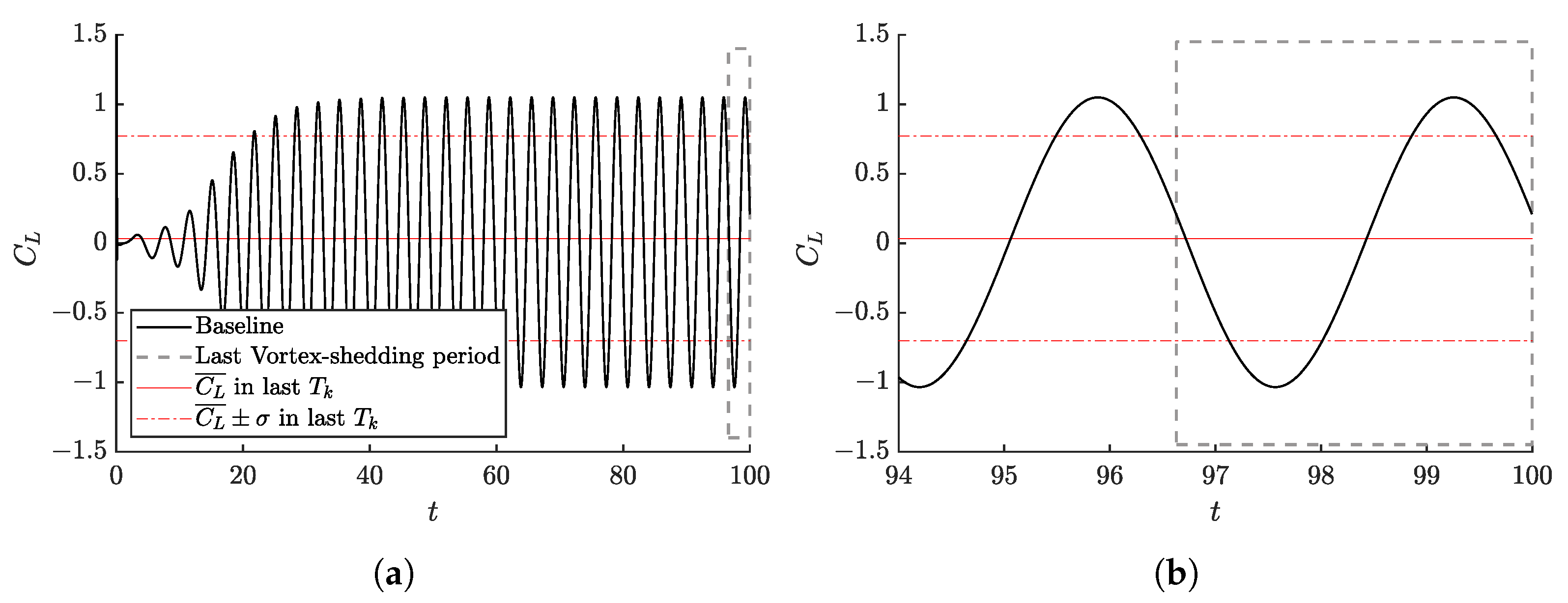
3.1. CFD and DRL Code Validation

As can be seen in the work by Rabault et al. [19], for a R e = 100 , through the correct actuation of the DRL, it was possible to achieve a decrease in the cylinder drag of 8%. These results were validated in other simulations, such as Li and Zhang [31], and applied in similar research [29,45,46].
Figure 7 shows eleven different “trainings” launched and the average C D obtained for the last vortex-shedding period of the different episodes. It can be seen that all cases follow the same learning trend, where most of the said learning is observed in the first hundred episodes. The main trend is obtained by adjusting a fourth-degree polynomial fit using the average coefficient data, and its purpose is to help to visualize the data. From this point on, the slope of the C D decrease is not so pronounced, reaching a stable solution for 350 episodes.
The obtained learning is then applied to the previously-shown baseline. To this end, one of the 11 trained agents is randomly selected and is run in a deterministic mode. This deterministic simulation is initiated from the conditions of the baseline case at 100 time units from the start. The C D and C L trends are shown in Figure 8, which indicates that a value of C D = 2.95 is obtained after applying the control, i.e., a decrease of 8.9% compared with the baseline case. The C D improvement is calculated as a function of the baseline C D :
improvement = 1 C D controlled C D baseline × 100 .
This result is rapidly achieved from the moment the control is applied. In the case of C L , the mean remains approximately at 0. However, the amplitude of the variation of this coefficient has been reduced, as shown by the lower standard deviation obtained. This may indeed have great beneficial consequences from the structural and stability points of view.
The control imposed on each jet is represented in Figure 9. As discussed above, the control starts at 100 time units of simulation, so the values of injected or suctioned mass prior to this time are null. Having imposed the synthetic-jet condition, everything injected by one jet (positive values) will be equivalent to what is suctioned by the other (negative values). In the first 10 time units approximately, the control of greater amplitude leads to a significant reduction in the drag, maximizing the reward. Next, the transitional control seeks to obtain a more stable actuation. After 25 time units, the solution is practically periodic.
More information about the control is obtained by observing the contours of instantaneous velocity and pressure for the controlled and uncontrolled cases, as shown in Figure 10. The DRL agent reduces C D by manipulating the wake vortex: it increases the size of the recirculation region and reduces both the frequency and the amplitude of the von Kármán street downstream of the cylinder. A similar conclusion is obtained from the instantaneous pressure field, which exhibits a decrease in the pressure maxima after applying the control. Comparing our results with those by Rabault et al. [19], it can be seen that the response of the control is practically the same except for very small differences that can come from the different numerical schemes to resolve the flow.
Increasing the Reynolds number also requires reducing the period of actuation, as mentioned in Section 2.2. Additionally, increasing the Reynolds number leads to a more complex flow, thus a higher number of episodes are expected to be necessary to complete the training. Therefore, parallelization using 20 environments has been adopted when simulating higher- R e cases. The parallelization using a multi-environment approach is fully detailed in the work of Rabault and Kuhnle [27].
In Figure 11, a comparison between employing a single environment and a 20 multi-environment approach is conducted for a case of R e = 1000 . It can be observed that if the Reynolds increases an order of magnitude, in this case, the number of episodes for the DRL to act to the same degree is three times greater using only one environment, as compared with Figure 7. The same solution can be obtained by parallelizing through 20 environments, using 50 episodes in each environment, which helps to reduce the real calculation time significantly.
As mentioned before, the flow is more complex, and its structures are less periodic and more chaotic. To analyze the flow, the instantaneous and average velocity fields are represented in Figure 12.
The obtained results are consistent with those of Ren et al. [32], which report an extensive flow analysis of the same Reynolds number. The control produces an elongation of the recirculation bubble behind the cylinder, reducing at the same time the hydrodynamic drag. For this Reynolds number, the control strategy found by the PPO agent is based on synchronous blowing. This strategy is similar to that found in lower Reynolds numbers: the jets produce an ejection or suction, generating a flow opposite to that caused by the wake.

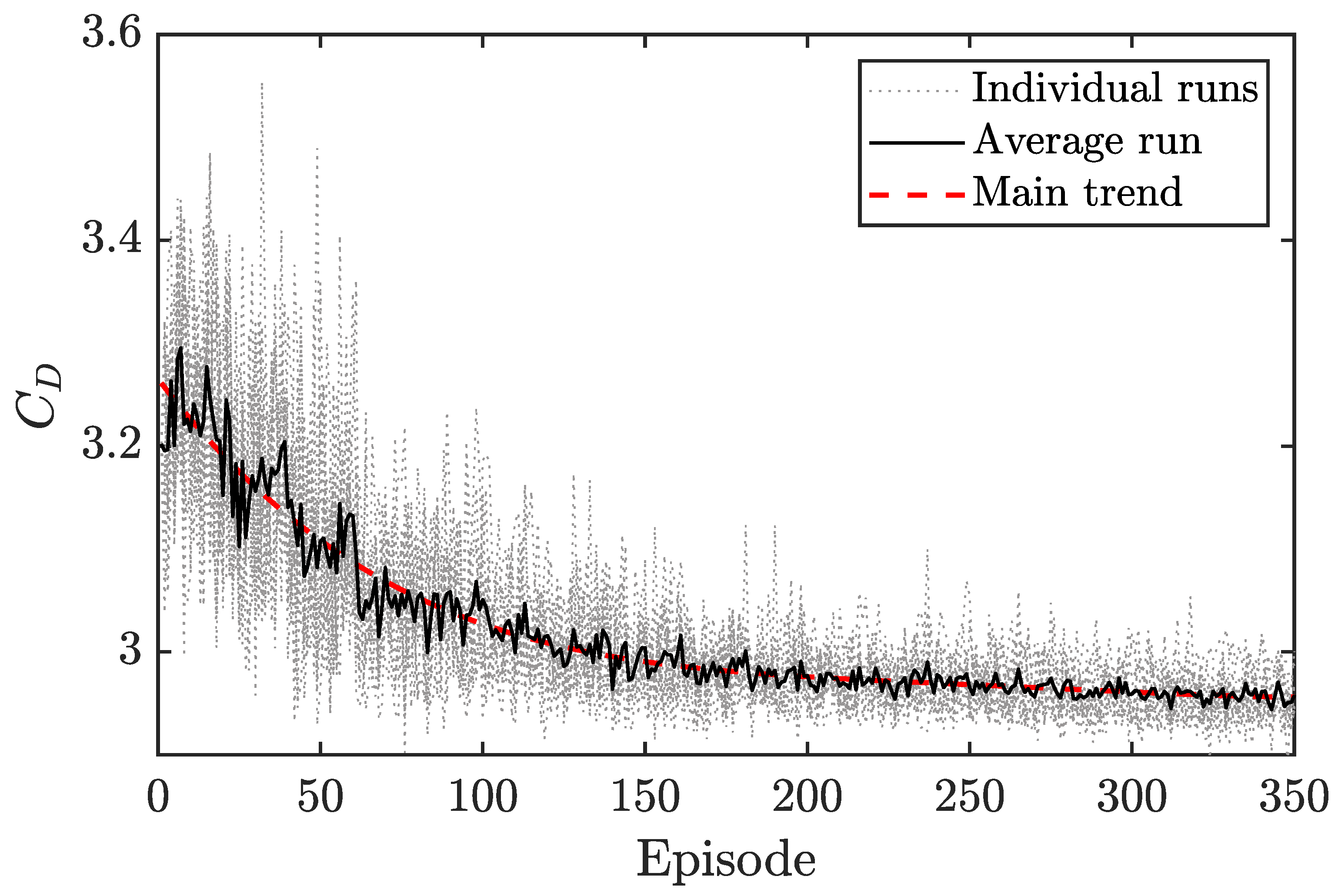
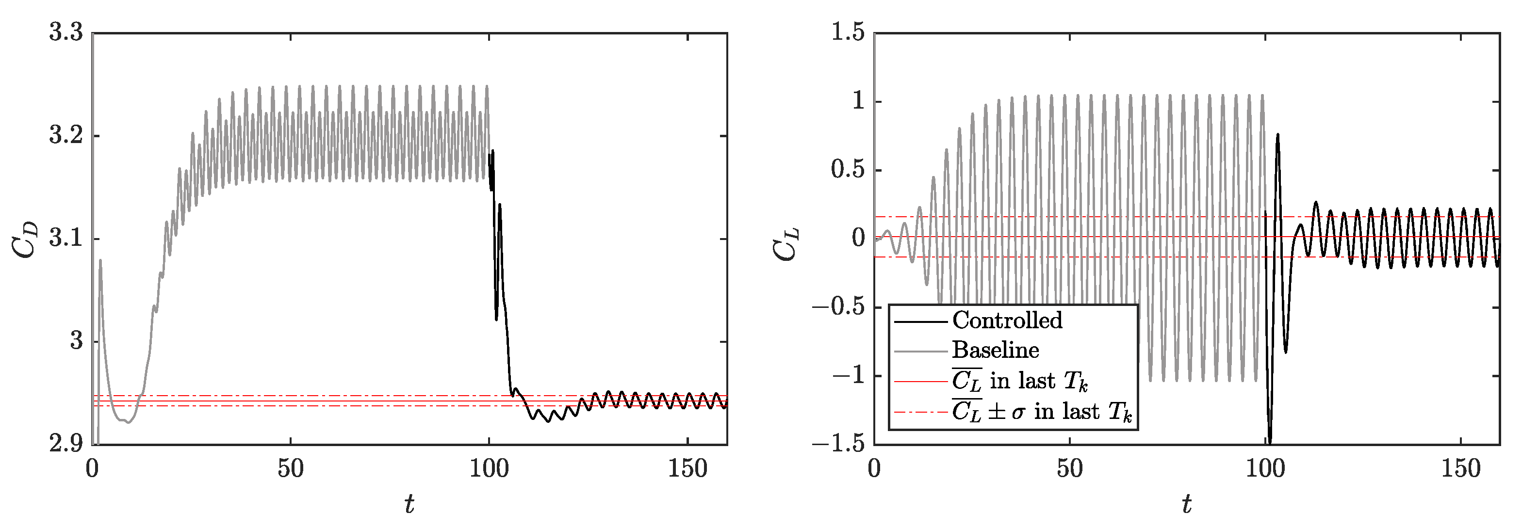
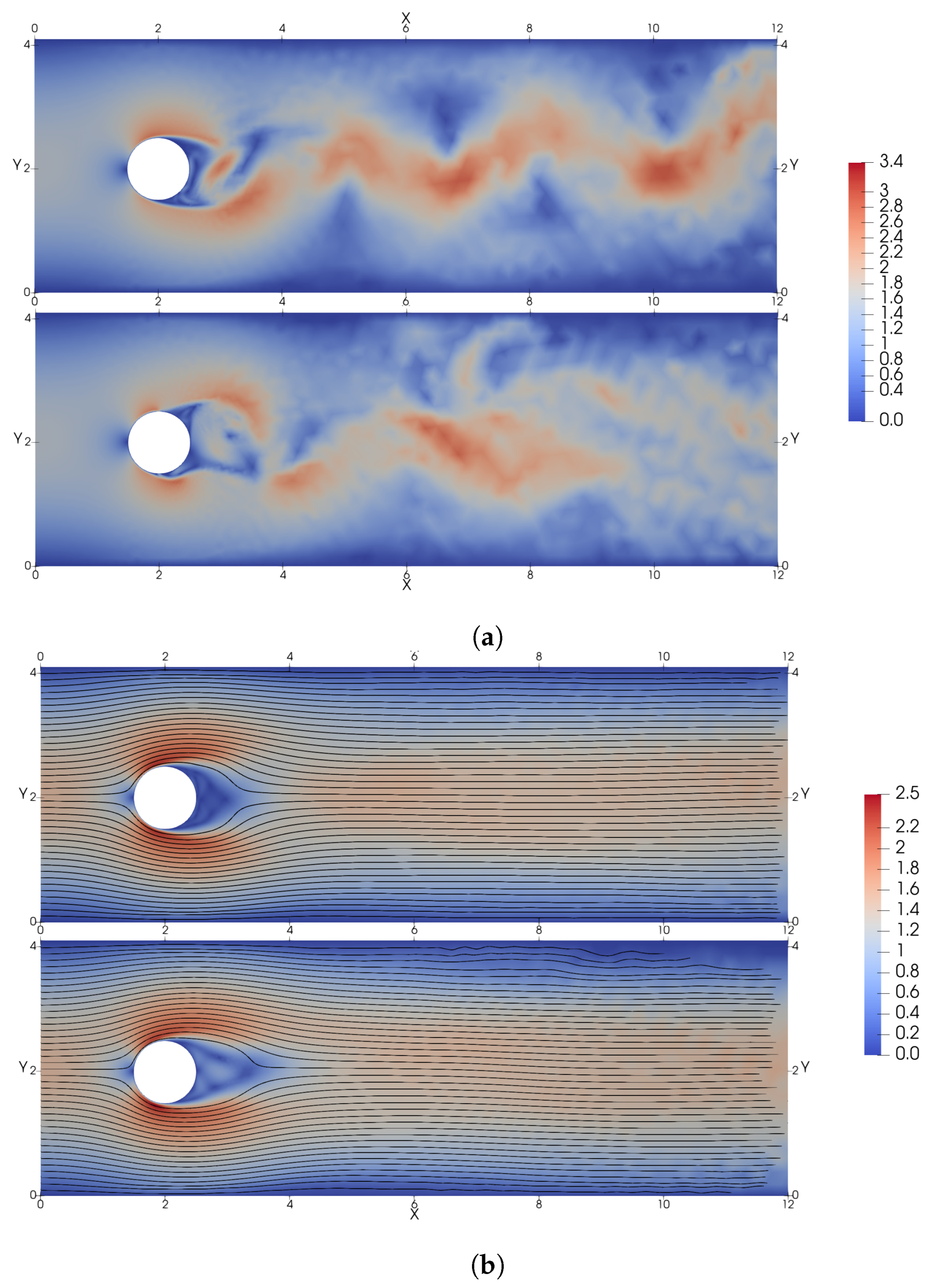
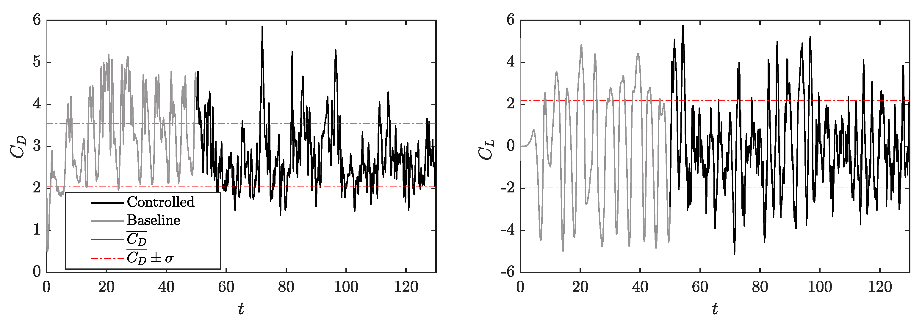
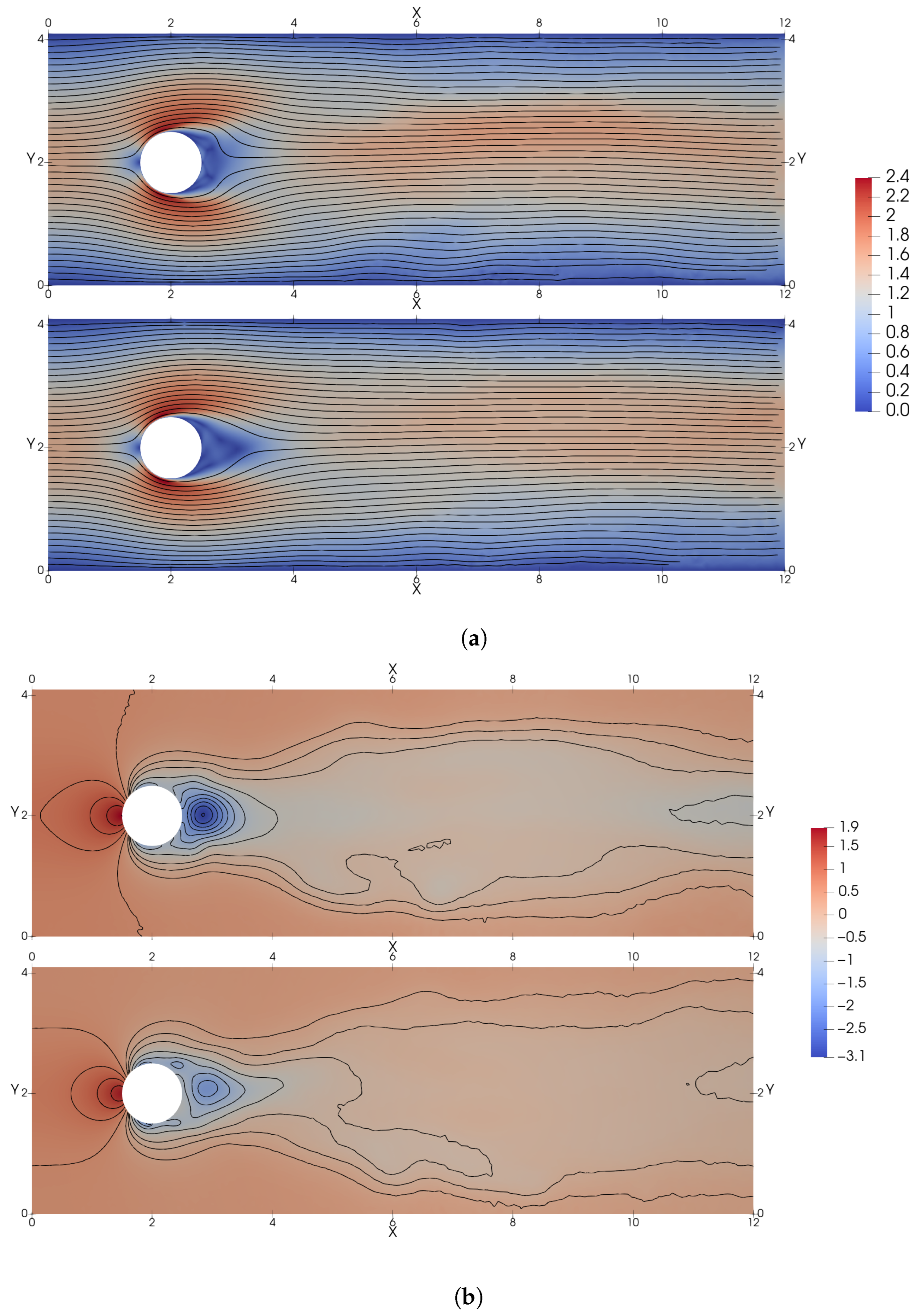
3.2. DRL Application at Reynolds Number 2000

Through the use of parallelization with a multi-environment strategy, even higher Reynolds numbers can be achieved. The results obtained for training with R e = 2000 are discussed below and, to the authors’ knowledge, there is no record of applying DRL control to such a high Reynolds number in the literature.
The C D and C L obtained through the application of learning in a deterministic mode are represented in Figure 13. This figure contrasts sharply with the one observed with R e = 100 (Figure 8). In this case, the starting baseline flow is much more chaotic, which can be seen in the magnitude of the peaks of both variables. The average drag coefficient of the non-controlled flow is C D = 3.39 . After the control, the average in this period is C D = 2.79 , which means more than 17% of C D improvement. In this case, it has been chosen to represent the mean in the entire controlled period and not during the last vortex-shedding since, as the solution behaves more erratically, it could lead to an average that is far from reality. Regarding the lift coefficient, the applied control manages to set the average C L with a close value to 0, maximizing the reward function as desired and avoiding a systematic biased strategy (see Appendix B in Rabault and Kuhnle [27]). Moreover, the absolute value of the peaks during the oscillating periods is reduced but not as much as in the case of Reynolds number 100, due to the chaotic nature of the flow at this higher Reynolds number.
In Figure 14 the average velocity and pressure fields are shown both for the baseline and the controlled deterministic case. As can be seen in the average velocity field comparison, the separation point in the controlled case is further downstream of the cylinder. This way, the average wake is narrowed faster in the controlled case, lowering the drag produced. This phenomenon is easier to observe if the difference between the baseline and the controlled case is considered as shown in Figure 15. This figure shows that the more significant difference between the controlled and uncontrolled cases occurs in the separation zone. At the same time, as observed for lower-Reynolds number control, the pressure drop behind the cylinder is reduced when controlled.
This control strategy is completely different from that used low at lower Reynolds numbers of values R e = 100 and 1000. In order to better understand this control strategy, a chronological velocity and pressure field snapshot is plotted in Figure 16. In this case, the control strategy does not involve the elongation of the recirculation bubble behind the cylinder. The flow separation is controlled and energized by a high-frequency actuation of the jets. The separation point is moved behind the cylinder lowering the drag of the cylinder, similar to the Eiffel paradox phenomenon, also known as the drag crisis, as defined by Stabnikov and Garbaruk [47]. The agent attempts to minimize the drag with this high frequency, breaking the vortices produced after the cylinder into smaller and less-energetic ones.
Additionally, one video (of the velocity and pressure fields) is shared to aid the visualization. The corresponding link can be found at the end of the document in the “Data Availability Statement”.

3.3. Cross-Application of Agents

Once the C D improvement results have been obtained for all the calculated Reynolds numbers thanks to the use of DRL, the cross-application of agents for a flow at R e = 2000 is studied.
Cross-application of agents involves applying a previously trained ANN with a different Reynolds number flow to solve a similar problem, using the achieved learning in other conditions. The final objective is to reduce the computational cost of training the DRL agent, since training an ANN with a lower Reynolds number is less expensive. This approach can be very beneficial as long as the results produced by the agent are comparable, i.e., the physics are similar enough between the two different cases.
Here it is investigated the drag reduction obtained by the agents previously trained for Reynolds numbers 100 and 1000 when they are applied in a deterministic mode to the flow of R e = 2000 , as can be seen in Figure 17.
The cross-application of the agent trained at R e = 100 does not yield a result that reduces drag in a flow at R e = 2000 . No drag improvement is obtained because the nature of the flow where the agent is applied is too different from the one where it was trained. However, when the trained agent at R e = 1000 is applied for the case of R e = 2000 , a significant drag reduction is produced. An average C D value of 2.74 is obtained, translating into a 19% drag reduction improvement compared with the baseline flow. This is a slightly larger drag reduction than that obtained by the agent trained at R e = 2000 . This small difference can be attributed to the chaotic nature of the flow, from evaluation run to evaluation run, and sub-optimal trade-off with respect to the actual reward function due to less good control of the lift and drag fluctuations, as will be discussed later. The fact that two similar results are obtained with different natures of control strategies, as explained in Section 3.2, may indicate that the flow at R e = 2000 belongs to a transition regime toward a higher Reynolds number flow, which only admits a high-frequency control in order to obtain the drag reduction. Therefore, being in this transition regime would admit both controls yielding comparable results. In order to go deep into this topic, higher Reynolds numbers must be simulated, but that goes beyond the scope of this article. At the same time, this is a doubly positive result since it confirms the fact that it is possible to apply deep-learning models previously trained at lower Reynolds number but within the same R e regime (similar dynamics) while saving time and computational resources [48].
The average C D comparisons for each agent used in the cross-application at R e = 2000 are shown in Figure 18 (left). As detailed in the previous section, the control strategy varies significantly as the Reynolds number increases. At R e = 100 and 1000, the control attempts to keep the recirculation bubble behind the cylinder, at R e = 2000 , high-frequency suction and blowing of the jets is applied to quickly force the flow transition, breaking the vortices into smaller ones. Despite these differences in the control strategies between the agents trained at R e = 1000 and 2000, both are capable to obtain a comparable drag reduction in a flow at R e = 2000 . As shown in Figure 18 (right), the C L bias obtained using the policy from R e = 1000 is higher than that obtained using the policy of R e = 2000 . Moreover, C L fluctuations are larger when employing the agent trained at R e = 1000 (not shown here for the sake of brevity). Note that the R e = 2000 strategy reduces the drag almost as much as using cross-application of agents and, at the same time, exhibits a slightly better performance in the lift; since the lift is part of the reward function, the agent trained at R e = 2000 achieves a higher reward at R e = 2000 than the agent trained at R e = 1000 . Nevertheless, the small differences between both "trainings" may be reversed for different baseline flows (changing the initial condition). This is similar to the results observed by Ren et al. [32].
In Figure 19, the average magnitude of velocity field at R e = 2000 is shown for the cross-application of the agent trained at R e = 1000 . At first glance, the existent bias in the average velocity field, which is directly linked with the asymmetric lift behavior, is noticeable.
In order to quantitatively observe the different control strategies, the power-spectral density (PSD) of the actions is plotted for the policy of R e = 2000 , and the cross-application of agents, R e = 1000 and 100, in Figure 20 (left). The latter two agents share the same strategy, which consists of a low-frequency action with no significant content at medium and high frequencies. In contrast, with the policy of R e = 2000 , the frequency spectrum is distributed, with a peak at a frequency of 1.1 . In Figure 20 (right), the frequency spectrum of the pressure at the probe in the detachment region indicated in Figure 3 is shown. A low frequency of 0.24 governs the baseline flow, corresponding to the vortex-shedding frequency. This frequency is mitigated by the policy of R e = 2000 in higher frequencies. Specifically, the frequency peak at 1.1 is a consequence of the corresponding actuation at this frequency, which is responsible for breaking the flow into smaller vortices as seen in Figure 16. On the other hand, it can be seen how the agent trained at R e = 1000 tends towards a completely different strategy in terms of frequency, actuating with a low-frequency strategy. The agent trained at R e = 100 , also uses this low-frequency actuation, but it does not have the capabilities to influence the pressure field. As mentioned before, in those cases, the agent attempts an opposition control strategy increasing the recirculation bubble to minimize the drag.

4. Conclusions

In this work, the high-performance CFD solver Alya was coupled with an ANN DRL agent to simulate and control the flow around a 2D cylinder with two jets attached to the cylinder surface. The main control objective was set on the reduction of the average drag. For the first time, the Reynolds number of the canonical 2D cylinder control problem from Rabault et al. [19] was extended to R e = 2000 , providing new insights into the DRL control strategies for highly complex and dynamic flows. Additionally, the R e = 100 and R e = 1000 cases were studied for validation and comparison purposes.
The most striking outcome of the R e = 2000 case is that the DRL agent uses a radically different strategy from those obtained at lower Reynolds numbers while still being able to provide a 17% drag reduction. In the new strategy, the agent attempts to delay the detachment point in the cylinder surface using a high-frequency signal in the actuation of the jets, similar to what can be observed in drag crisis phenomena. It is shown that the cylinder wake is narrowed by the breakdown of the detaching vortices into smaller structures. This strategy contrasts with the one obtained at a lower Reynolds number, where the agent acts at a lower frequency to perform opposition control and to elongate the recirculation bubble behind the cylinder. These results are further verified with the spectral analysis of the jet actuating signals and a pressure witness point in the wake. Table 2 summarizes the results from this paper and provides an overview of the results in previous works. Information about drag reduction, the control strategy, and the configuration of the jet location is also provided.
The applications of agents trained at R e = 100 and R e = 1000 on the R e = 2000 case were investigated (namely cross-applications). It was shown that the R e = 100 agent is not able to reduce the drag in the high Reynolds number regime due to the different dynamics of the system. On the other hand, the R e = 1000 provides satisfactory results, which even beat the R e = 2000 agent itself ( 19% drag reduction), even though the mean wake displays an asymmetric pattern in this case, which corresponds to an overall reward (including lift bias penalization) that is lower than with the agent trained at R e = 2000 . Still, this opens up the door to accelerating the training of an agent by first exposing it to a lower Reynolds number flow, which demands a lower computational effort, and then finalize the training at the target Reynolds number condition.
As a final observation, the actual time that the agent takes to calculate the output action once it receives the input state is negligible for an ANN consisting of 2 layers of 512 neurons each, and it could be considered instantaneous. Therefore, it will be completely possible to implement these schemes in real time. In the experiments, there can be some non-negligible delay times depending on the hardware systems used in the experiment. However, if the training is performed in the same conditions, i.e., the delay is also present during the training, the agent will learn a strategy that works under such circumstances. In addition, if the agent is trained in a numerical environment and applies it on the experimental side, then the state sent as an input must consider the known delay in the experiment.

Author Contributions

Conceptualisation: R.V., J.R. and O.L.; investigation: all authors; data curation: P.V., P.S., F.A.-Á., A.M., J.R. and B.F.; software: J.R., A.M., B.F. and O.L.; writing—original draft: P.V., P.S. and F.A.-Á.; editing: all authors; funding: L.M.G.-C., O.L. and R.V. All authors have read and agreed to the published version of the manuscript.

Funding

Pau Varela is partially supported through a grant for the mobility of doctoral students provided by Universitat Politècnica de València and the program Erasmus Prácticas E+ 2020-1. R.V. acknowledges funding from the ERC through grant no. “2021-CoG-101043998, DEEPCONTROL”.

Institutional Review Board Statement

Not applicable.

Informed Consent Statement

Not applicable.

Data Availability Statement

The data presented in this study are available upon request from the corresponding author. The YouTube link to “Deep reinforcement learning for flow control on a cylinder at Re = 2000” is https://youtu.be/8R3adCQmeEA, accessed on 28 November 2022.

Acknowledgments

The authors acknowledge the contribution of Maxence Deferrez to this work. R.V. acknowledges funding from the ERC through grant no. “2021-CoG-101043998, DEEPCONTROL”.

Conflicts of Interest

The authors declare no conflict of interest. The funders had no role in the design of the study; in the collection, analyses, or interpretation of data; in the writing of the manuscript, or in the decision to publish the results.

Abbreviations

The following abbreviations are used in this manuscript:
Abbreviations
AFCactive flow control
ANNartificial neural network
BSC-CNSBarcelona Supercomputing Center—Centro Nacional de Supercomputación
CFDcomputational fluid dynamics
CFLCourant–Friedrichs–-Lewy
CPUcentral processing unit
DRLdeep reinforcement learning
EMACenergy-, momentum-, and angular-momentum-conserving equation
FEMfinite-element method
HPChigh-performance computing
PPOproximal policy optimization
PSDpower-spectral density
UAVunmanned aerial vehicle
Roman letters
aaction
C L lift coefficient
C D drag coefficient
C offset offset coefficient of the reward
Dcylinder diameter
e j vector used in force calculation
fexternal forces, frequency
f k vortex shedding frequency
FForce
F D drag force
F L lift force
Hchannel height
Lchannel length
nunit vector normal to the cylinder
Qmass flow rate
Q * normalized mass flow rate
Q ref reference mass flow rate
ppressure
rreward
r norm reference value of the reward after control
Rcylinder radius
R e Reynolds number
Ssurface
sobservation state
s norm reference pressure in the observation state
S t Strouhal number
ttime
t 0 initial time
t f final time
T a action period
T k vortex-shedding period
uflow speed
U ¯ mean velocity
U in inlet boundary velocity in x direction
U max inlet boundary velocity in the middle of the channel
V in inlet boundary velocity in y direction
v i jet velocity
wlift penalization
xhorizontal coordinate
yvertical coordinate
Greek letters
ϵ velocity strain-rate tensor
ν kinematic viscosity
Ω domain
ω jet angular opening
ρ density
σ standard deviation
ς Cauchy stress tensor
θ jet angle
θ 0 center jet angle

References

  1. Howell, J.P. Aerodynamic Drag Reduction for Low Carbon Vehicles; Woodhead Publishing Limited: Sawston, UK, 2012; pp. 145–154. [Google Scholar] [CrossRef]
  2. Bechert, D.W.; Bartenwerfer, M. The viscous flow on surfaces with longitudinal ribs. J. Fluid Mech. 1989, 206, 105–129. [Google Scholar] [CrossRef]
  3. Gad-el Hak, M. Active, and Reactive Flow Management; Cambridge University Press: Cambridge, UK, 2000. [Google Scholar] [CrossRef]
  4. Guerrero, J.; Sanguineti, M.; Wittkowski, K. CFD Study of the Impact of Variable Cant Angle Winglets on Total Drag Reduction. Aerospace 2018, 5, 126. [Google Scholar] [CrossRef] [Green Version]
  5. Tiseira, A.O.; García-Cuevas, L.M.; Quintero, P.; Varela, P. Series-hybridisation, distributed electric propulsion and boundary layer ingestion in long-endurance, small remotely piloted aircraft: Fuel consumption improvements. Aerosp. Sci. Technol. 2022, 120, 107227. [Google Scholar] [CrossRef]
  6. Serrano, J.R.; García-Cuevas, L.M.; Bares Moreno, P.; Varela Martínez, P. Propeller Position Effects over the Pressure and Friction Coefficients over the Wing of an UAV with Distributed Electric Propulsion: A Proper Orthogonal Decomposition Analysis. Drones 2022, 6, 38. [Google Scholar] [CrossRef]
  7. Serrano, J.R.; Tiseira, A.O.; García-Cuevas, L.M.; Varela, P. Computational Study of the Propeller Position Effects in Wing-Mounted, Distributed Electric Propulsion with Boundary Layer Ingestion in a 25 kg Remotely Piloted Aircraft. Drones 2021, 5, 56. [Google Scholar] [CrossRef]
  8. Kametani, Y.; Fukagata, K. Direct numerical simulation of spatially developing turbulent boundary layers with uniform blowing or suction. J. Fluid Mech. 2011, 681, 154–172. [Google Scholar] [CrossRef] [Green Version]
  9. Fan, Y.; Atzori, M.; Vinuesa, R.; Gatti, D.; Schlatter, P.; Li, W. Decomposition of the mean friction drag on an NACA4412 airfoil under uniform blowing/suction. J. Fluid Mech. 2022, 932, A31. [Google Scholar] [CrossRef]
  10. Atzori, M.; Vinuesa, R.; Schlatter, P. Control effects on coherent structures in a non-uniform adverse-pressure-gradient boundary layer. Int. J. Heat Fluid Flow 2022, 97, 109036. [Google Scholar] [CrossRef]
  11. Atzori, M.; Vinuesa, R.; Stroh, A.; Gatti, D.; Frohnapfel, B.; Schlatter, P. Uniform blowing and suction applied to nonuniform adverse-pressure-gradient wing boundary layers. Phys. Rev. Fluids 2021, 6, 113904. [Google Scholar] [CrossRef]
  12. Fahland, G.; Stroh, A.; Frohnapfel, B.; Atzori, M.; Vinuesa, R.; Schlatter, P.; Gatti, D. Investigation of Blowing and Suction for Turbulent Flow Control on Airfoils. AIAA J. 2021, 4422–4436. [Google Scholar] [CrossRef]
  13. Voevodin, A.V.; Kornyakov, A.A.; Petrov, A.S.; Petrov, D.A.; Sudakov, G.G. Improvement of the take-off and landing characteristics of wing using an ejector pump. Thermophys. Aeromech. 2019, 26, 9–18. [Google Scholar] [CrossRef]
  14. Yousefi, K.; Saleh, R. Three-dimensional suction flow control and suction jet length optimization of NACA 0012 wing. Meccanica 2015, 50, 1481–1494. [Google Scholar] [CrossRef]
  15. Cui, W.; Zhu, H.; Xia, C.; Yang, Z. Comparison of Steady Blowing and Synthetic Jets for Aerodynamic Drag Reduction of a Simplified Vehicle; Elsevier B.V.: Amsterdam, The Netherlands, 2015; Volume 126, pp. 388–392. [Google Scholar] [CrossRef] [Green Version]
  16. Park, H.; Cho, J.H.; Lee, J.; Lee, D.H.; Kim, K.H. Experimental study on synthetic jet array for aerodynaic drag reduction of a simplified car. J. Mech. Sci. Technol. 2013, 27, 3721–3731. [Google Scholar] [CrossRef]
  17. Choi, H.; Moin, P.; Kim, J. Active turbulence control for drag reduction in wall-bounded flows. J. Fluid Mech. 1994, 262, 75–110. [Google Scholar] [CrossRef]
  18. Muddada, S.; Patnaik, B.S. An active flow control strategy for the suppression of vortex structures behind a circular cylinder. Eur. J. Mech. B/Fluids 2010, 29, 93–104. [Google Scholar] [CrossRef]
  19. Rabault, J.; Kuchta, M.; Jensen, A.; Réglade, U.; Cerardi, N. Artificial neural networks trained through deep reinforcement learning discover control strategies for active flow control. J. Fluid Mech. 2019, 865, 281–302. [Google Scholar] [CrossRef] [Green Version]
  20. Ghraieb, H.; Viquerat, J.; Larcher, A.; Meliga, P.; Hachem, E. Optimization and passive flow control using single-step deep reinforcement learning. Phys. Rev. Fluids 2021, 6. [Google Scholar] [CrossRef]
  21. Pino, F.; Schena, L.; Rabault, J.; Mendez, M. Comparative analysis of machine learning methods for active flow control. arXiv 2022, arXiv:2202.11664. [Google Scholar]
  22. Garnier, P.; Viquerat, J.; Rabault, J.; Larcher, A.; Kuhnle, A.; Hachem, E. A review on deep reinforcement learning for fluid mechanics. Comput. Fluids 2021, 225, 104973. [Google Scholar] [CrossRef]
  23. Rabault, J.; Ren, F.; Zhang, W.; Tang, H.; Xu, H. Deep reinforcement learning in fluid mechanics: A promising method for both active flow control and shape optimization. J. Hydrodyn. 2020, 32, 234–246. [Google Scholar] [CrossRef]
  24. Vinuesa, R.; Brunton, S.L. Enhancing computational fluid dynamics with machine learning. Nat. Comput. Sci. 2022, 2, 358–366. [Google Scholar] [CrossRef]
  25. Vinuesa, R.; Lehmkuhl, O.; Lozano-Durán, A.; Rabault, J. Flow Control in Wings and Discovery of Novel Approaches via Deep Reinforcement Learning. Fluids 2022, 7, 62. [Google Scholar] [CrossRef]
  26. Belus, V.; Rabault, J.; Viquerat, J.; Che, Z.; Hachem, E.; Reglade, U. Exploiting locality and translational invariance to design effective deep reinforcement learning control of the 1-dimensional unstable falling liquid film. AIP Adv. 2019, 9, 125014. [Google Scholar] [CrossRef] [Green Version]
  27. Rabault, J.; Kuhnle, A. Accelerating deep reinforcement learning strategies of flow control through a multi-environment approach. Phys. Fluids 2019, 31, 094105. [Google Scholar] [CrossRef] [Green Version]
  28. Tang, H.; Rabault, J.; Kuhnle, A.; Wang, Y.; Wang, T. Robust active flow control over a range of Reynolds numbers using an artificial neural network trained through deep reinforcement learning. Phys. Fluids 2020, 32, 053605. [Google Scholar] [CrossRef]
  29. Tokarev, M.; Palkin, E.; Mullyadzhanov, R. Deep reinforcement learning control of cylinder flow using rotary oscillations at low reynolds number. Energies 2020, 13, 5920. [Google Scholar] [CrossRef]
  30. Xu, H.; Zhang, W.; Deng, J.; Rabault, J. Active flow control with rotating cylinders by an artificial neural network trained by deep reinforcement learning. J. Hydrodyn. 2020, 32, 254–258. [Google Scholar] [CrossRef]
  31. Li, J.; Zhang, M. Reinforcement-learning-based control of confined cylinder wakes with stability analyses. J. Fluid Mech. 2022, 932, A44. [Google Scholar] [CrossRef]
  32. Ren, F.; Rabault, J.; Tang, H. Applying deep reinforcement learning to active flow control in weakly turbulent conditions. Phys. Fluids 2021, 33, 037121. [Google Scholar] [CrossRef]
  33. Wang, Q.; Yan, L.; Hu, G.; Li, C.; Xiao, Y.; Xiong, H.; Rabault, J.; Noack, B.R. DRLinFluids: An open-source Python platform of coupling deep reinforcement learning and OpenFOAM. Phys. Fluids 2022, 34, 081801. [Google Scholar] [CrossRef]
  34. Qin, S.; Wang, S.; Rabault, J.; Sun, G. An application of data driven reward of deep reinforcement learning by dynamic mode decomposition in active flow control. arXiv 2021, arXiv:2106.06176. [Google Scholar]
  35. Vazquez, M.; Houzeaux, G.; Koric, S.; Artigues, A.; Aguado-Sierra, J.; Aris, R.; Mira, D.; Calmet, H.; Cucchietti, F.; Owen, H.; et al. Alya: Towards Exascale for Engineering Simulation Codes. arXiv 2014, arXiv:1404.4881. [Google Scholar]
  36. Owen, H.; Houzeaux, G.; Samaniego, C.; Lesage, A.C.; Vázquez, M. Recent ship hydrodynamics developments in the parallel two-fluid flow solver Alya. Comput. Fluids 2013, 80, 168–177. [Google Scholar] [CrossRef] [Green Version]
  37. Lehmkuhl, O.; Houzeaux, G.; Owen, H.; Chrysokentis, G.; Rodriguez, I. A low-dissipation finite element scheme for scale resolving simulations of turbulent flows. J. Comput. Phys. 2019, 390, 51–65. [Google Scholar] [CrossRef]
  38. Charnyi, S.; Heister, T.; Olshanskii, M.A.; Rebholz, L.G. On conservation laws of Navier–Stokes Galerkin discretizations. J. Comput. Phys. 2017, 337, 289–308. [Google Scholar] [CrossRef] [Green Version]
  39. Charnyi, S.; Heister, T.; Olshanskii, M.A.; Rebholz, L.G. Efficient discretizations for the EMAC formulation of the incompressible Navier–Stokes equations. Appl. Numer. Math. 2019, 141, 220–233. [Google Scholar] [CrossRef] [Green Version]
  40. Crank, J.; Nicolson, P. A practical method for numerical evaluation of solutions of partial differential equations of the heat-conduction type. Adv. Comput. Math. 1996, 6, 207–226. [Google Scholar] [CrossRef]
  41. Trias, F.X.; Lehmkuhl, O. A self-adaptive strategy for the time integration of navier-stokes equations. Numer. Heat Transf. Part B Fundam. 2011, 60, 116–134. [Google Scholar] [CrossRef]
  42. Kuhnle, A.; Schaarschmidt, M.; Fricke, K. Tensorforce: A TensorFlow Library for Applied Reinforcement Learning. 2017. Available online: https://tensorforce.readthedocs.io (accessed on 28 November 2022).
  43. Abadi, M.; Agarwal, A.; Barham, P.; Brevdo, E.; Chen, Z.; Citro, C.; Corrado, G.S.; Davis, A.; Dean, J.; Devin, M.; et al. TensorFlow: Large-Scale Machine Learning on Heterogeneous Systems. 2015. Available online: tensorflow.org (accessed on 28 November 2022).
  44. Schäfer, M.; Turek, S.; Durst, F.; Krause, E.; Rannacher, R. Benchmark Computations of Laminar Flow Around a Cylinder; Vieweg+Teubner Verlag: Wiesbaden, Germany, 1996; pp. 547–566. [Google Scholar] [CrossRef]
  45. Elhawary, M. Deep reinforcement learning for active flow control around a circular cylinder using unsteady-mode plasma actuators. arXiv 2020, arXiv:2012.10165. [Google Scholar]
  46. Han, B.Z.; Huang, W.X.; Xu, C.X. Deep reinforcement learning for active control of flow over a circular cylinder with rotational oscillations. Int. J. Heat Fluid Flow 2022, 96, 109008. [Google Scholar] [CrossRef]
  47. Stabnikov, A.; Garbaruk, A. Prediction of the drag crisis on a circular cylinder using a new algebraic transition model coupled with SST DDES. J. Phys. Conf. Ser. 2020, 1697, 012224. [Google Scholar] [CrossRef]
  48. Guastoni, L.; Güemes, A.; Ianiro, A.; Discetti, S.; Schlatter, P.; Azizpour, H.; Vinuesa, R. Convolutional-network models to predict wall-bounded turbulence from wall quantities. J. Fluid Mech. 2021, 928, A27. [Google Scholar] [CrossRef]
Figure 1. Main domain dimensions in terms of the cylinder diameter D, where ω represents the jet width and θ 0 is the angle of the center of the jet. In light blue, the parabolic velocity profile of the inlet and the jet are represented. The domain representation is not to scale.
Actuators 11 00359 g001
Figure 2. Computational grid used for the R e = 100 calculations.
Actuators 11 00359 g002
Figure 3. Schematic representation of the computational domain, where the red dots correspond to the location of the probes. The position of two probes is remarked as black dots for further analysis in Section 3.3.
Actuators 11 00359 g003
Figure 4. Flow rate of the jet Q smoothed and applied in the numerical simulation (green) versus the discrete Q decided by the DRL agent (red).
Actuators 11 00359 g004
Figure 5. Temporal evolution of the lift coefficient in the baseline case (without jet actuation). (a) Baseline lift-coefficient results. The vortex-shedding period is 3.37 time units. (b) Zoom-in view of the vortex-shedding period in the baseline case.
Actuators 11 00359 g005
Figure 6. General overview of the DRL-CFD (computational fluid dynamics) framework employed in this work. A multi-environment approach was used to parallelize the learning and speed up training.
Actuators 11 00359 g006
Figure 7. Evolution of C D in the last vortex-shedding period as a function of the episode.
Actuators 11 00359 g007
Figure 8. Temporal evolution of C D (left) and C L (right) obtained through the application of the DRL control (at t = 100 ), run in a deterministic mode, for R e = 100 .
Actuators 11 00359 g008
Figure 9. Flow rate through each jet as a function of time after applying the DRL control.
Actuators 11 00359 g009
Figure 10. Instantaneous flow fields at R e = 100 , where for each pair of images, the baseline case without control is depicted on the top and the controlled case is depicted on the bottom. (a) Instantaneous magnitude of the velocity fields. (b) Instantaneous pressure fields.
Actuators 11 00359 g010
Figure 11. Evolution of C D in the last vortex-shedding for each episode employing a single environment (left) or a 20-multi-environment approach (right) showing the learning curve indexed by the episode number for one of the 20 environments.
Actuators 11 00359 g011
Figure 12. Instantaneous and average flow fields at R e = 1000 , where for each pair of images, the baseline case without control is depicted on the top and the controlled case is depicted on the bottom. (a) Instantaneous magnitude of velocity fields. (b) Average magnitude of velocity fields, where the mean streamlines are indicated in black.
Actuators 11 00359 g012
Figure 13. Temporal evolution of C D (left) and C L (right) obtained through the application of the DRL control (at t = 50 ), run in a deterministic mode, for R e = 2000 .
Actuators 11 00359 g013
Figure 14. Average flow fields at R e = 2000 , where each pair of images, the baseline case without control is depicted on the top and the controlled case is depicted on the bottom. (a) Average magnitude of velocity fields. (b) Average pressure fields.
Actuators 11 00359 g014
Figure 15. Difference in the mean flow fields at R e = 2000 , between the controlled and baseline case. (a) Difference in the mean magnitude of velocity fields. (b) Difference in mean pressure fields.
Actuators 11 00359 g015
Figure 16. Magnitude of the velocity (left) and pressure (right) field progression at R e = 2000 . The control starts at t = 50 , therefore the first two panels of each column correspond to the uncontrolled case and the rest (involving smaller vortices) correspond to the controlled flow.
Actuators 11 00359 g016
Figure 17. Temporal evolution of C D obtained through cross-application of agents trained at R e = 100 (left) and R e = 1000 (right) in a deterministic mode to a case with a Reynolds number of 2000.
Actuators 11 00359 g017
Figure 18. Average C D (left) and average C L (right) comparison between three different cross-application of agents.
Actuators 11 00359 g018
Figure 19. Average flow fields at R e = 2000 , using the training obtained for R e = 1000 .
Actuators 11 00359 g019
Figure 20. Power-spectral density of the action output, Q, for the R e = 2000 case, with its own policy and two cross-application policies (left) and for pressure in the probe near the cylinder in the separation zone (right).
Actuators 11 00359 g020
Table 1. Parameters of the simulations for each Reynolds number considered in this work.
Re 10010002000
Mesh cells (approximately)11,00019,00052,000
Number of witness points151151151
| Q | max 0.0880.040.04
s norm 1.722
C offset 3.173.293.29
r norm 51.251.25
w0.211
T k 3.373.044.39
T a 0.250.20.2
Actions per episode80100100
Number of episodes35010001400
CPUs per environment464646
Environments11 or 2020
Total CPUs4646 or 920920
Baseline duration100250100
Table 2. Summary of the results and strategies. In the strategy, column E states the elongation of the bubble of recirculation and D states the delay of the detachment point through a high-frequency actuation. Note that for the four cases of Tang et al. [28], a unique agent is trained through transfer learning for all four Reynolds numbers and jets have small x-velocity components.
Re WorkCD ReductionStrategyConfiguration
100Present work 8.9 % E2 jets (1 top & 1 bottom)
100Rabault et al. [19] 8 % E2 jets (1 top & 1 bottom)
100Tang et al. [28] 5.7 % E4 jets (2 top & 2 bottom)
200Tang et al. [28] 21.6 % E4 jets (2 top & 2 bottom)
300Tang et al. [28] 32.7 % E4 jets (2 top & 2 bottom)
400Tang et al. [28] 38.7 % E4 jets (2 top & 2 bottom)
1000Present work 20.0 % E2 jets (1 top & 1 bottom)
1000Ren et al. [32] 30 % E2 jets (1 top & 1 bottom)
2000Present work 17.7 % D2 jets (1 top & 1 bottom)
Publisher’s Note: MDPI stays neutral with regard to jurisdictional claims in published maps and institutional affiliations.

