
Electrohydraulic and Electromechanical Buoyancy Change Device Unified Vertical Motion Model


1
INEGI, Faculdade de Engenharia, Universidade do Porto, Rua Dr. Roberto Frias, s/n, 4200-465 Porto, Portugal
2
Faculdade de Engenharia, Universidade do Porto, Rua Dr. Roberto Frias, 400, 4200-465 Porto, Portugal
3
INESC TEC, Faculdade de Engenharia, Universidade do Porto, Rua Dr. Roberto Frias, 4200-465 Porto, Portugal
*
Author to whom correspondence should be addressed.
Actuators 2023, 12(10), 380; https://doi.org/10.3390/act12100380
Submission received: 20 August 2023
/
Revised: 20 September 2023
/
Accepted: 3 October 2023
/
Published: 8 October 2023
(This article belongs to the Section Control Systems)
Abstract
:Depth control is crucial for underwater vehicles, not only to perform certain tasks that require the vehicle to be still at a given depth but also because most propeller-driven vehicles waste a considerable amount of energy to counteract the passively tuned positive buoyancy. The use of a variable buoyancy system (VBS) can effectively address these items, increasing the energetic efficiency and thus mission length. Achieving accurate depth controllers is, however, a complex task, since experimental controller development in sea or even in test pools is unpractical and the use of simulation requires accurate vertical motion models whose parameters might be difficult to obtain or measure. The development of simple, yet comprehensive, dynamic models for devices incorporating VBS is therefore of upmost importance, as well as developing procedures that allow a simple determination of their parameters. This work contributes to this field by deriving a unified model for the vertical motion of a VBS actuated device, irrespective of the specific technological actuation solution employed, whether it be electromechanical or electrohydraulic. A concise analysis of the open-loop stability of the unified model is presented and a straightforward yet efficient procedure for identifying several of its parameters is introduced. This identification procedure is designed to be convenient and can be carried out in shallow waters, such as test pools, while its results are applicable to the deeper water model as well. To validate the procedure, experimental values obtained from an electromechanical VBS actuated device are used. Closed-loop control of the electromechanical VBS actuated device is conducted through simulation and experimental tests. The results confirm the effectiveness of the proposed unified model and the parameter identification methodology.
1. Introduction
In recent decades, ocean monitoring and exploration have become increasingly vital, driven by a combination of scientific and economic factors. This improved significance has underscored the demand for enhanced precision and durability in equipment, enabling a sustained human presence in marine environments. The advancement of submersible vehicles stands out as a prominent trend in this domain, offering superior survivability compared to their surface counterparts. Furthermore, economic interests are driving the development of submersible vehicles since it is estimated that there are significant mineral resources at the bottom of the sea [1,2]. Although the majority of commercial unmanned underwater robots are connected with tethers and operated remotely (the remotely operated vehicles, ROV), their application is restricted due to substantial operational expenses, among other factors [1]. Given the scenario described above and the limitations of ROV, there is an increasing demand for cutting-edge underwater autonomous robot technologies.
Research in this field has been rich with different studies addressing the vehicle structure [3], namely by incorporating shape-optimized and bio-mimetic components to decrease drag and increase the energetic efficiency [4,5,6,7]. A relevant issue in this field is the difficulty found in underwater communications. Recent trends [3] are the use of wireless optical communication [8,9] and hybrid acoustic and RF communication [10]. Navigation and control are also important topics of research in this area. Current developments in navigation and motion planning include neural networks, computer vision and image recognition to develop less expensive object detection, obstacle avoidance [11] and visual odometry systems [12,13]. Present day advancements in vehicle control include the use of sliding mode [14], fuzzy [15] and neural network [16,17] controllers to cope with the highly nonlinear behavior of the vehicle dynamics.
Variable buoyancy systems (VBS) play a crucial role in developing the functionality and efficiency of underwater robotics [18,19]. By adjusting their buoyancy, these systems enable underwater vehicles to control their depth in water, mimicking the natural behavior of marine creatures. This capability is particularly significant in various applications such as marine exploration, underwater inspections and environmental monitoring. By utilizing variable buoyancy, underwater robots can achieve precise positioning and stabilization, enabling them to navigate complex underwater environments with ease.
Another important aspect is the conservation of energy and extended operational endurance. By utilizing variable buoyancy devices, underwater vehicles may minimize energy expenditure when moving through water or when remaining stationary for long periods [20], therefore conserving battery life, and thus extending their operational duration. This is especially valuable in scientific research or exploration missions where prolonged periods of data collection or monitoring are necessary.
In order to take advantage of the benefits that a variable buoyancy system may provide, a suitable controller should be devised. The controller might be tuned to increase performance, whenever the task requires accurate depth control, like for instance when performing underwater filming tasks [21] or detecting seismic ocean waves [22], or on energy saving, whenever the goal is to extend the mission duration, like for instance in tasks requiring the inspection of long-distance water tunnels [23]. Despite the particular focus of the control task, an accurate dynamic model of the system is of upmost importance to develop the controller. In fact, experimentally developing controllers is challenging and often impractical due to the high costs and time required for conducting pool tests or sea trials. Although several studies in the literature present experimental and simulation results of depth control in vehicles using buoyancy change devices [22,24,25,26,27,28], the accuracy of the model, namely for depth control purposes, is usually discarded. For instance, in [22], the model of an electrohydraulic VBS vertical motion is developed and used to synthesize several linear and nonlinear controllers. However, no experimental validation of the model is provided. In [24], the vertical motion model of an electromechanical VBS is modelled and used in simulation to tune a PD controller. Once again, no direct experimental validation of the model is presented. In [25], the mathematical dynamic model for a deep-sea electrohydraulic buoy is established, accounting for the pressure hull deformation and the current disturbances on the vertical motion. A finite-time boundedness (FTB) depth control strategy is then developed and simulated on the proposed model of the buoy. Although sea experimental closed-loop control results are presented, there appears to be a considerable difference between the results predicted with the model and the ones obtained experimentally. In [26], depth controllers for the vertical motion of a variable buoyancy module are developed. The controllers are developed based on a complete model of the system comprehending actuator dynamics and vertical motion dynamics. Although the authors of [26] state that the model parameters were determined through rigorous experimentation, no presentation of such experimental procedures is provided and no experimental validation of the model is presented. In [27], the vertical motion model of a low-cost autonomous profiling float, able to dive up to 50 m, is developed and used to devise a state-feedback depth controller. The model does not include actuator dynamics. Since some of the model parameters are hard to determine, an Extended Kalman Filter is used to estimate some of the model parameters. Experimental results show accurate control performance, but once again no comparison between model simulation and experimental results is provided.
As can be seen from the description above, many works in the literature use the vertical motion model of a VBS to develop the controller in simulation, but there is not any comparison between the experimental and simulated results. A notable exception may be found in [28], where an electromechanical actuated VBS is developed for incorporation in a hybrid aerial underwater vehicle. In this work, a complete motion 3D model is developed, and the pitch angle and heave velocity simulation results obtained in closed-loop control using a PID controller are compared against the ones obtained in lake experiments. The model does not comprehend, however, the actuator dynamics, and there is no experimental procedure to determine the model parameters. This is of particular importance given that the vertical motion requires many parameters that might be difficult to experimentally determine or to obtain from manufacturer’s datasheets. Although an observer could be used to estimate such parameters, following a strategy similar to the one in [27], such a strategy involves more computing power and complexity of the control law.
This paper is an evolution of a previous work by the authors [29] where the dynamic model of an electromechanical actuated VBS model was devised and experimentally identified. The main novel contributions of this paper are the following: (i) it is shown that a unified model for the vertical motion of a VBS can be found, regardless of the technological actuation solution used, electromechanical or electrohydraulic. The focus is exclusively on the vertical motion component, assuming that the device is either a float without pitch and roll characteristics or that these variables are managed with other vehicle actuators; (ii) the open-loop stability of the unified model is briefly analyzed and a simple, yet effective, procedure to identify several of the unified model parameters is proposed. For convenience, this procedure was designed to be performed in shallow waters (for example, in test pools), although its results are appliable to the deeper water model; (iii) the procedure is validated through experimental values obtained using an electromechanical VBS; and (iv) closed-loop control of an electromechanical VBS is performed both in simulation and experimentally. Results validate the proposed unified model and the parameter identification methodology.
The paper is organized as follows: Section 2 presents the dynamic model of the vertical motion of a VBS actuated device. This section starts by presenting the detailed actuation models for the motor in Section 2.1.1 and electrohydraulic and electromechanical solutions in Section 2.1.2 and Section 2.1.3, respectively. Then, in Section 2.1.4, a unified actuation model is presented. The model presented in Section 2.1.4 is combined with the submerged device dynamics leading to the overall vertical motion model in Section 2.2. The model devised in Section 2.2 is then simplified in Section 2.3 to be able to determine its parameters in a shallow water experimental procedure. In Section 2.4, the model determined in Section 2.2 is rewritten as a function of the parameters determined in Section 3.1. Section 2.5 presents a concise analysis of the open-loop stability of the model presented in Section 2.4. Section 3 presents the experimental results obtained in the model identification procedure, as well as the ones obtained in closed-loop control. A comparison between these results and the ones obtained in simulation is also provided.
2. Dynamic Model of the Vertical Motion of a VBS Actuated Device
2.1. Actuation System Model
As presented in Section 1, many solutions to implement the actuator element of a VBS can be found in the literature. However, the majority of them are either (a) an electrohydraulic solution, consisting of a motor driving a pump inserting/retrieving a nearly incompressible fluid in/from a flexible volume or (b) an electromechanical solution, consisting of a linear actuator pushing/retracting a piston. These two solutions can be described with the scheme presented in Figure 1, where the hydraulic transmission is a pump, the mechanical transmission is typically a gearbox and a spindle and the mechanical converter is a bladder or a piston.
2.1.1. Motor Model
In this work, it will be assumed that the motor driving either the electromechanical or electrohydraulic solutions is a voltage-driven permanent magnet DC motor, for which the model presented in Figure 2 applies [30]:
In Figure 2, R is the coils’ resistance, L is the coils’ inductance, kT is the current to torque gain, kemf is the back electromotive force gain, Jm is the inertia of the rotor, Bm is a coefficient describing the torque losses proportional to motor velocity, is a torque representing losses due to motor viscous friction, brushes’ friction and eddy currents, is the motor torque, is an external torque and and are the motor acceleration, velocity and angular position, respectively.
Since the electrical dynamics are much faster than the mechanical dynamics of the motor, they will be neglected in this work. In this case, the model reduces to the following model, presented in Figure 3:
Where , relating the applied voltage with the stall torque , and is the total torque decrease with velocity.
2.1.2. Electrohydraulic Solution Model
The typical electrohydraulic circuit used in VBS comprehends a motor driving a pump and a piston or bladder, with possibly a pressure amplifier, as depicted in Figure 4. The amplifier has a gain of , where can generically be higher or lower than one and A1 and A2 are the areas defined in Figure 4. It is typically desired that the pump operating pressure is lower than the sea pressure, so that .
Hydraulic valves are omitted from this circuit as it is assumed that they do not impose significant pressure drops.
Using the mass conservation principle, the pressure evolution inside the oil chamber can be written as follows [31]:
where is the volumetric flow from/to the pump, is the volume of the chamber connected to the pump and is the oil effective isothermal bulk modulus (accounting for trapped air). For a mineral oil at 5 MPa, the bulk modulus is approximately Pa [32]. For this example, the relative variation of volume for a pressure variation, , of 10 MPa (corresponding to a working depth of 1000 m) would be very small, as shown below:
Based on the assumption that the oil is essentially incompressible, the inertia of the hydraulic transmission and of the pressure amplifier/reducer may be lumped into the inertia of the motor whose model is depicted in Figure 3. By doing so, the model of the electrohydraulic actuation system can be represented as in the block diagram of Figure 5.
In the diagram of Figure 5, is the motor speed, is the torque the motor has to surpass due to the increase in pressure with depth, is the inertia of the motor plus the reflected inertia on the motor of the pump, moving oil, piston and added mass of the displaced water, is a parameter equal to the sum of with a term representing pump and piping viscous friction, V is the volume displaced using the piston or bladder and is a constant relating the change in buoyancy force with the change in the volume (assuming that water density is essentially constant). Also, the leakage-caused volume change can be written as
where is the leakage flow of the pump, assumed to be proportional using the factor to the pump operating pressure:
can therefore be written as
where is the leakage coefficient defined with
In the diagram of Figure 5, the influence of the depth on the motor torque, denoted with , is characterized using the factor , which can be written as
where is the pump displacement, is the mechanical efficiency of the pump and is the ratio between areas defined above.
Finally, can be written as
2.1.3. Electromechanical Solution Model
A typical electromechanical solution comprehends an electrical motor, a mechanical reducer and a spindle, as depicted in Figure 6.
In this case, since the mechanical transmission stiffness is very high, the moving masses of both the mechanical reducer and the piston can be lumped into the electrical motor inertia, leading to the block diagram of Figure 7.
Where is the inertia of the motor plus the reflected inertia on the motor of the mechanical reducer, spindle, piston and added mass of the displaced water, is a parameter equal to the sum of with a term representing mechanical transmission viscous friction, is a constant accounting for the transmission ratio between the force exerted with the outside pressure and the corresponding torque caused on the motor, is the transmission efficiency, is the area of the piston in contact with sea water, is the transmission pitch and . All other remaining variables are defined as in Figure 5.
2.1.4. Unified Model for the Actuation System of the VBS
Comparing the block diagrams of Figure 5 and Figure 7, it is possible to check that in both cases, there is a second-order, type-one transfer function between the voltage applied to the motor and the buoyancy change. The model of the actuator part of the VBS can therefore be defined generically as in Figure 8:
Where the several constants and variables are resumed in Table 1.
For the block diagram presented in Figure 8, the transfer function between the control action and the volume V(s) is given with
It is clear from the analysis of transfer function (9). that the volume of the piston is affected by the depth at which the VBS is. This means that if the controller of V(s) is not able to fully reject the disturbance caused by Z(s), the depth of the VBS will affect, with a negative sign, V(s). As it will be seen in the next section, this means that if the controller is not able to fully reject Z(s), then positive feedback will occur, making the system unstable.
2.2. Overall Vertical Motion Model of the VBS Actuated Device
In this work, it will be assumed that the device is either a float, for which pitch and roll do not exist, or that these variables are controlled with other vehicle actuators. Consequently, the free body diagram of a buoyancy change device with overall structure and added masses m can be represented schematically as in Figure 9. Two of the forces appearing in this diagram have the same value and opposite signs: the forces , due to the weight of the vehicle, and , the buoyancy force caused by the immersed volume at its equilibrium position (which is trimmed to compensate for the vehicle weight). is the buoyancy force caused by changing the immersed volume and , the hydrodynamic drag force, assumed to be proportional to the square of the vehicle velocity [25]. Finally, is the buoyancy force caused by the relative variation of the vehicle hull and sea water volumes with pressure, which can be written as [27].
Applying Newton’s second law to the VBS device, according to Figure 9, leads to the following equation, where denotes the prototype depth:
By considering Equation (10) and the ones resulting from the block diagram of Figure 8, Equations (11)–(13) can be found. Equations (11) and (12) derive directly from the block diagram of Figure 8 and Equation (13) can be obtained by rewriting Equation (10) using the definitions of and previously presented at the beginning of this section. The block diagram corresponding to these equations is detailed in Figure 10.
Equations (11) and (12) can be further collapsed into Equation (14), leading to the following model:
where is the drag force defined as
where is a parameter defining the transition between laminar and turbulent flow regimes, characterized, respectively, with and . From a control perspective, it is interesting to have a linearized model around an equilibrium point corresponding to small vehicle vertical velocities. In this case, the flow regime is laminar, so that Equations (17) and (18) apply:
Applying the Laplace transform to Equations (17) and (18), transfer functions (19) and (20) can be found, where, as expected, transfer function (19) is similar to transfer function (9) as they both represent the actuator dynamics:
2.3. Simplified Model for Parameter Identification in Shallow Water
In order to fully know the model represented in Equations (19) and (20), a total of nine parameters is required. Some of those parameters might be difficult to determine because they are not directly measurable and/or the manufacturer does not provide their values. In this section, the model presented in Equations (19) and (20) will be rewritten so that a simple experimental procedure to determine its parameters can be derived. This procedure is meant to be used, for convenience, in shallow waters, although the parameters determined from it are still valid for the deeper water model. This procedure is based on rewriting the model as two first-order transfer functions, one between and and one between and . As will be presented in the following, this allows four of the model parameters to be directly estimated with simple shallow water experiments. The remaining five parameters can be either measured, retrieved from the manufacturer’s datasheets or estimated using basic physics laws.
For shallow waters, the values of and can be neglected, since the value of is low. Applying this simplification to the block diagram of Figure 10 leads to the following transfer function between and :
The transfer function (21) can be rewritten as
where
and
Using the same reasoning as above, for shallow waters, the force can be neglected in the block diagram of Figure 10. The transfer function between and in this situation simplifies to
The transfer function (25) can be rewritten as
or
where
2.4. Overall Vertical Motion Model with Identification Parameters
The parameters of the model determined in the previous section can be identified at low depths. However, for control purposes, for instance, it is useful to have a model that is valid at any depth. Rewriting Equation (20) using the coefficients defined in the previous section leads to Equation (30).
In Equation (30), from Equation (28) and can be written as follows [27]:
where (m3/m) is a parameter expressing the loss of volume per meter depth due to the relative variation of volume of the prototype’s structure compared to the comparable one of water, under the same pressure. Using this information, (30) can be further written as
Rewriting Equation (19) using the coefficients determined in the previous section leads to Equation (33):
2.5. Open-Loop Stability Analysis
Combining Equations (32) and (33) leads to the open-loop transfer function between the applied voltage and the VBS depth:
According to the Routh [33] criterion, the open-loop system is unstable. In fact, given that all parameters of the transfer function are positive, at least two of the coefficients of the characteristic equation are negative.
One interesting conclusion that can be made from the analysis of transfer function (34) is that, contrary to what has been described in the literature, even if is negative, which happens whenever the effect of the increase in water density with pressure is higher than the decrease in volume of the VBS device due to pressure, the system remains unstable due to and .
An interesting case occurs when considering that
- , which is expected in the electromechanical solution, and might be acceptable if a high volumetric efficient pump is used in the electrohydraulic solution;
- , by assuming that the device structure compressibility is exactly counterbalanced with the increase in water density with pressure;
- , by assuming that the outside pressure does not influence the velocity and position of the actuator (for instance, if the controller is able to fully reject the disturbance caused by the VBS depth in Equation (33)).
Under these circumstances, the system model can be written as
Equation (35) shows that the system becomes a fourth-order type-two system. It is still, however, an unstable system, since its phase margin is negative.
3. Experimental Results
The prototype used for the experimental results presented in this section is presented in Figure 11.
It is a prototype of an electromechanical VBS capable of diving up to 100 m and with a maximum volume change of cm3. Its full length is 1285 mm with an outer radius of 200 mm. The prototype displaced volume is Vp = 0.0275 m3 when the movable piston is at its central position. Its dry weight is 33 kg, so approximately 5.5 dm3 of extra floatation was added to make the prototype neutrally buoyant at that equilibrium situation. More details on the VBS and its control unit can be found in [29].
3.1. Model Identification Results
The steady state values and time constants of transfer functions (22) and (26) can be estimated using two simple experiments that can be performed in shallow waters: in order to identify the parameters of (22), the VBS is actuated with different voltage steps, corresponding to different steady state velocities of the piston motion. Voltages and velocities (estimated using centered finite differences applied, in post processing, to the piston displacement sensor data) are registered so that the parameters of (22) are identified. This procedure was presented in detail in [29], for an electromechanical VBS, leading to the following results: mm·s−1·V−1 and s.
In order to identify the parameters of (26), the variable volume of the VBS is changed to different values around the one corresponding to neutral buoyancy, so that different terminal velocities of the prototype are achieved. Imposed volumes and vehicle depth velocities are registered so that the parameters of (26) are identified. In order to be able to do this in shallow waters while ensuring that the identification steps start from a neutral buoyancy situation, the following procedure is developed in this work:
- Starting from the bottom, and using closed-loop control, control the depth of the vehicle until it reaches nearly zero velocity around , where should be conveniently chosen, according to the vehicle length, in order to ensure that it is neither touching the bottom nor partially emerged (see step (d) below). When this happens, the vehicle is at its zero-buoyancy setting. Please notice that the dynamic and steady state closed-loop characteristics obtained with the controller used at this stage (and at stage (c)) are essentially irrelevant, as the only purpose is to make the vehicle reach a nearly zero velocity. For this reason, the controller to be used in this step can have a coarse tuning;
- Stop closed-loop control, and increase the buoyancy by a factor of . In the particular case of the prototype presented in Figure 11, this is equivalent to increasing the piston position by a constant value . This was made in an open loop, by using the information provided by the manufacturer regarding the steady state relation between applied voltage and actuator speed. Having that information, the time that a given voltage should be applied to reach a desired position can be easily calculated. Wait until the vehicle reaches the bottom while recording the value of its depth z;
- Using closed-loop control, control the depth of the vehicle until it reaches nearly zero velocity around When this happens, the vehicle is at its zero buoyancy setting;
- Stop closed-loop control, and decrease the buoyancy by a factor of . Again, in the particular case of the prototype presented in Figure 11, this is equivalent to decreasing the piston position by a constant value, . Wait until the vehicle reaches the bottom, while recording the value of its depth z.
The procedure outlined above was used to identify the parameters of Equation (26) for the prototype presented in Figure 11. The procedure was run four times, corresponding to eight experiments, each with a different value of , ±≈2.5 mm, ±≈4 mm, ±≈6 mm and ±≈10 mm, corresponding to the following values of ±≈20 cm3, ±≈30 cm3, ±≈45 cm3 and ±≈75 cm3. Results of the evolution of the depth z are presented in Figure 12, along with the identification of steps (a) to (d) presented above for the first run.
Results of the piston position X, depth Z and depth velocity dZ/dt from steps (b) and (d) were then used to identify open-loop transfer function (26), from V () to Z and (21) from V to dZ/dt. The average parameters obtained are presented in Table 2. These parameters are very close, validating the proposed approach. Using the average values of Table 2 for each parameter, the measured and predicted values for dZ/dt and for Z are presented in Figure 13 and Figure 14, respectively, for each experiment.
3.2. Control Results
The model presented in Equations (32) and (33), with the parameters identified in the previous section, was used to tune a cascaded controller, according to the block diagram presented in Figure 15.
Regarding Equation (33), K1 and T1 were identified in [29], for the prototype considered in this work and .
Regarding Equation (32), the parameter was estimated by considering that there is a loss of volume at a 100 m depth of 1% of the original prototype volume Vp due to hull compression. In this case, . K2 and T2 of Equation (32) are found in Section 3.1.
In this work, a proportional controller is used for , while a PID controller is used for . The controller parameters for the vehicle dynamics were heuristically tuned using the Matlab PID tuner toolbox. The controller was tuned to have a slightly underdamped behaviour, in order to avoid excessive oscillations that might cause energy waste. The controller that was obtained was implemented in the Arduino controlling the DFC actuator, running at a sampling period of 0.3 s, according to Equations (36) and (37). Table 3 resumes the parameters that were used at the experimental trials.
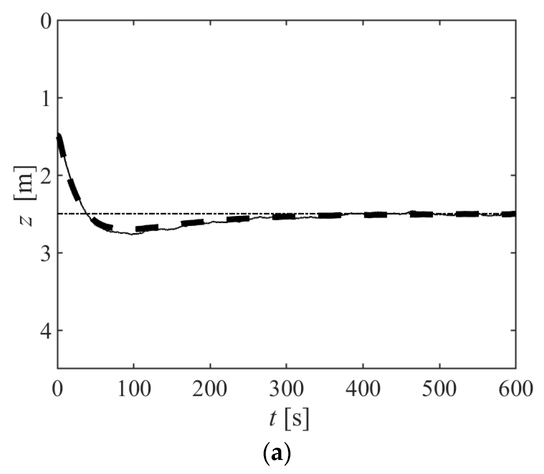
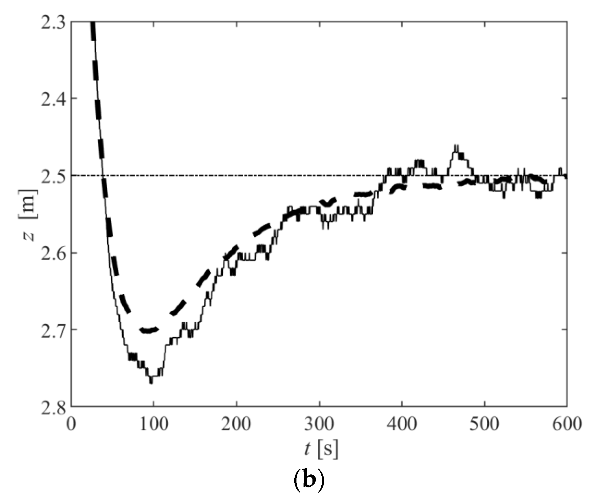
In order to test the performance of the actuator and validate the model presented in the previous sections, a series of experimental trials was performed in a 4.5 m depth pool. These trials consisted of a series of steps between different depths as shown in Figure 16. This figure shows not only the experimental evolution of depth of the VBS actuated device but also the one predicted with the model developed in Section 2.4. As can be seen, the overall prediction is very good, although a slight tendency to predict lower overshoots, especially in ascending steps, can be noticed. Finally, a longer trial was performed (Figure 17), to show that the device converges to the target depth with a neglectable error.
4. Conclusions and Future Work
This paper presented the model of the vertical motion of a variable buoyancy actuated device. Starting from the derivation of the models for electrohydraulic and electromechanical solutions, a unified model, independent of the actuation technology, was proposed. This model was then rewritten in a simplified way so that its parameters can be directly estimated with simple shallow water experiments. An experimental procedure for such experiments was proposed and tested. This procedure may be applied, for convenience, in shallow waters, although the identified parameters are also usable in the model that is valid for deeper waters. Both the modelling approach and the identification procedure were experimentally validated using an electromechanical actuated VBS, previously developed by the authors. In fact, experimental results show that the closed-loop model predictions match the measured ones with good accuracy. Future work will focus on (i) the development of a thruster actuated device, to obtain an experimental energetic comparison between the use of thrusters and the use of a VBS, (ii) a theoretical analysis of the closed-loop stability and (iii) development of a prototype for deeper waters (1000 m), allowing the experimental validation of the models developed in this work for greater depths.
Author Contributions
Conceptualization, J.F.C., F.G.d.A. and N.A.C.; methodology, J.F.C., F.G.d.A. and N.A.C.; software, J.B.P.; investigation, J.F.C., F.G.d.A. and N.A.C.; writing— J.F.C.; writing—review and editing, J.F.C., J.B.P., F.G.d.A. and N.A.C. All authors have read and agreed to the published version of the manuscript.
Funding
This work was financially supported through contract LAETA—UIDB/50022/2020 by “Fundação para a Ciência e Tecnologia”, which the authors gratefully acknowledge.
Data Availability Statement
Not applicable.
Conflicts of Interest
The authors declare no conflict of interest.
References
- Yuh, J. Design and develop of an autonomous underwater vehicle: A survey. Auton. Robot 2000, 8, 7–24. [Google Scholar] [CrossRef]
- Toro, N.; Robles, P.; Jeldres, R. Seabed mineral resources, an alternative for the future of renewable energy: A critical review. Ore Geol. Rev. 2020, 126, 103699. [Google Scholar] [CrossRef]
- Sahoo, A.; Dwivedy, S.K.; Robi, P.S. Advancements in the field of autonomous underwater vehicle. Ocean Eng. 2019, 181, 145–160. [Google Scholar] [CrossRef]
- Katzschmann, R.K.; DelPreto, J.; MacCurdy, R.; Rus, D. Exploration of underwater life with an acoustically controlled soft robotic fish. Sci. Robot. 2018, 3, eaar3449. [Google Scholar] [CrossRef] [PubMed]
- Nguyen, N.-D.; Choi, H.-S.; Tran, N.-H.; Kim, S.-K. Development of Ray-Type Underwater Glider. In Proceedings of the AETA 2017—Recent Advances in Electrical Engineering and Related Sciences: Theory and Application, Ho Chi Minh, Vietnam, 7–9 December 2018; pp. 677–685. [Google Scholar]
- Sun, C.; Song, B.; Wang, P.; Wang, X. Shape optimization of blended-wing-body underwater glider by using gliding range as the optimization target. Int. J. Nav. Archit. Ocean Eng. 2017, 9, 693–704. [Google Scholar] [CrossRef]
- Alam, K.; Ray, T.; Anavatti, S.G. Design and construction of an autonomous underwater vehicle. Neurocomputing 2014, 142, 16–29. [Google Scholar] [CrossRef]
- Oubei, H.M.; Shen, C.; Kammoun, A.; Zedini, E.; Park, K.-H.; Sun, X.; Liu, G.; Kang, C.H.; Ng, T.K.; Alouini, M.-S.; et al. Light based underwater wireless communications. Jpn. J. Appl. Phys. 2018, 57, 08PA06. [Google Scholar] [CrossRef]
- Sharifzadeh, M.; Ahmadirad, M. Performance analysis of underwater wireless optical communication systems over a wide range of optical turbulence. Opt. Commun. 2018, 427, 609–616. [Google Scholar] [CrossRef]
- Soomro, M.; Azar, S.N.; Gurbuz, O.; Onat, A. Work-in-Progress: Networked Control of Autonomous Underwater Vehicles with Acoustic and Radio Frequency Hybrid Communication. In Proceedings of the 2017 IEEE Real-Time Systems Symposium (RTSS), Paris, France, 5–8 December 2017; pp. 366–368. [Google Scholar]
- Lin, Y.-H.; Shou, K.-P.; Huang, L.-J. The initial study of LLS-based binocular stereo-vision system on underwater 3D image reconstruction in the laboratory. J. Mar. Sci. Technol. 2017, 22, 513–532. [Google Scholar] [CrossRef]
- Hildebrandt, M.; Kirchner, F. IMU-aided stereo visual odometry for ground-tracking AUV applications. In Proceedings of the OCEANS’10 IEEE SYDNEY, Sydney, NSW, Australia, 24–27 May 2010; pp. 1–8. [Google Scholar]
- Sukvichai, K.; Wongsuwan, K.; Kaewnark, N.; Wisanuvej, P. Implementation of visual odometry estimation for underwater robot on ROS by using RaspberryPi 2. In Proceedings of the 2016 International Conference on Electronics, Information, and Communications (ICEIC), Danang, Vietnam, 27–30 January 2016; pp. 1–4. [Google Scholar]
- Vo, T.Q.; Kim, H.S.; Lee, B.R. A study on turning motion control of a 3-joint fish robot using sliding mode based controllers. In Proceedings of the ICCAS 2010, Gyeonggi, Republic of Korea, 27–30 October 2010; pp. 1556–1561. [Google Scholar]
- Kato, N.; Ito, Y.; Kojima, J.; Takagi, S.; Asakawa, K.; Shirasaki, Y. Control performance of autonomous underwater vehicle “AQUA EXPLORER 1000” for inspection of underwater cables. In Proceedings of the Proceedings of OCEANS’94, Brest, France, 13–16 September 1994; Volume 131, pp. I/135–I/140. [Google Scholar]
- Wang, Z.; Guo, S.; Shi, L.; Pan, S.; He, Y. The application of PID control in motion control of the spherical amphibious robot. In Proceedings of the 2014 IEEE International Conference on Mechatronics and Automation, Tianjin, China, 3–6 August 2014; pp. 1901–1906. [Google Scholar]
- Li, J.H.; Lee, P.M. A neural network adaptive controller design for free-pitch-angle diving behavior of an autonomous underwater vehicle. Robot. Auton. Syst. 2005, 52, 132–147. [Google Scholar] [CrossRef]
- Falcão Carneiro, J.; Bravo Pinto, J.; Gomes de Almeida, F.; Cruz, N.A. Design and Experimental Tests of a Buoyancy Change Module for Autonomous Underwater Vehicles. Actuators 2022, 11, 254. [Google Scholar] [CrossRef]
- Zhang, Z.; Liu, B.; Wang, L. Autonomous underwater vehicle depth control based on an improved active disturbance rejection controller. Int. J. Adv. Robot. Syst. 2019, 16, 1729881419891536. [Google Scholar] [CrossRef]
- Carneiro, J.F.; Pinto, J.B.; Almeida, F.G.; Cruz, N.A. Variable Buoyancy or Propeller-Based Systems for Hovering Capable Vehicles: An Energetic Comparison. IEEE J. Ocean. Eng. 2020, 46, 414–433. [Google Scholar] [CrossRef]
- Love, T.; Toal, D.; Flanagan, C. Buoyancy Control for an Autonomous Underwater Vehicle. IFAC Proc. Vol. 2003, 36, 199–204. [Google Scholar] [CrossRef]
- Huang, H.; Zhang, C.; Ding, W.; Zhu, X.; Sun, G.; Wang, H. Design of the Depth Controller for a Floating Ocean Seismograph. J. Mar. Sci. Eng. 2020, 8, 166. [Google Scholar] [CrossRef]
- Qi, Y.; Wu, X.; Zhang, G.; Sun, Y. Energy-Saving Depth Control of an Autonomous Underwater Vehicle Using an Event-Triggered Sliding Mode Controller. J. Mar. Sci. Eng. 2022, 10, 1888. [Google Scholar] [CrossRef]
- Bai, Y.; Hu, R.; Bi, Y.; Liu, C.; Zeng, Z.; Lian, L. Design and Depth Control of a Buoyancy-Driven Profiling Float. Sensors 2022, 22, 2505. [Google Scholar] [CrossRef]
- Qiu, Z.; Wang, Q.; Li, H.; Yang, S.; Li, X. Depth Control for a Deep-Sea Self-Holding Intelligent Buoy Under Ocean Current Disturbances Based on Finite-Time Boundedness Method. IEEE Access 2019, 77, 114670–114684. [Google Scholar] [CrossRef]
- Ranganathan, T.; Singh, V.; Thondiyath, A. Theoretical and Experimental Investigations on the Design of a Hybrid Depth Controller for a Standalone Variable Buoyancy System—vBuoy. IEEE J. Ocean. Eng. 2018, 45, 414–429. [Google Scholar] [CrossRef]
- Mezo, T.; Maillot, G.; Ropert, T.; Jaulin, L.; Ponte, A.; Zerr, B. Design and control of a low-cost autonomous profiling float. Mech. Ind. 2020, 21, 512. [Google Scholar] [CrossRef]
- Hu, R.; Lu, D.; Xiong, C.; Lyu, C.; Zhou, H.; Jin, Y.; Wei, T.; Yu, C.; Zeng, Z.; Lian, L. Modeling, characterization and control of a piston-driven buoyancy system for a hybrid aerial underwater vehicle. Appl. Ocean Res. 2022, 120, 102925. [Google Scholar] [CrossRef]
- Carneiro, J.F.; Pinto, J.B.; Almeida, F.G.d.; Cruz, N.A. Model Identification and Control of a Buoyancy Change Device. Actuators 2023, 12, 180. [Google Scholar] [CrossRef]
- Moritz, F.G. Electromechanical Motion Systems—Design and Simulation; John Wiley & Sons: Hoboken, NJ, USA, 2014. [Google Scholar]
- Merritt, H. Hydraulic Control Systems; John Wiley & Sons: New York, NY, USA, 1967. [Google Scholar]
- Murrenhoff, H. Fundamentals of Fluid Power. Part 1: Hydraulics, 8th ed.; IFAS Institute fur Fluidtechnische Antriebe and Steuerungen: Aachen, Germany, 2016. [Google Scholar]
- Ogata, K. Modern Control Engineering, 5th ed.; Pearson: London, UK, 2009. [Google Scholar]
Figure 1.
Generic diagram of the actuator elements in a VBS.
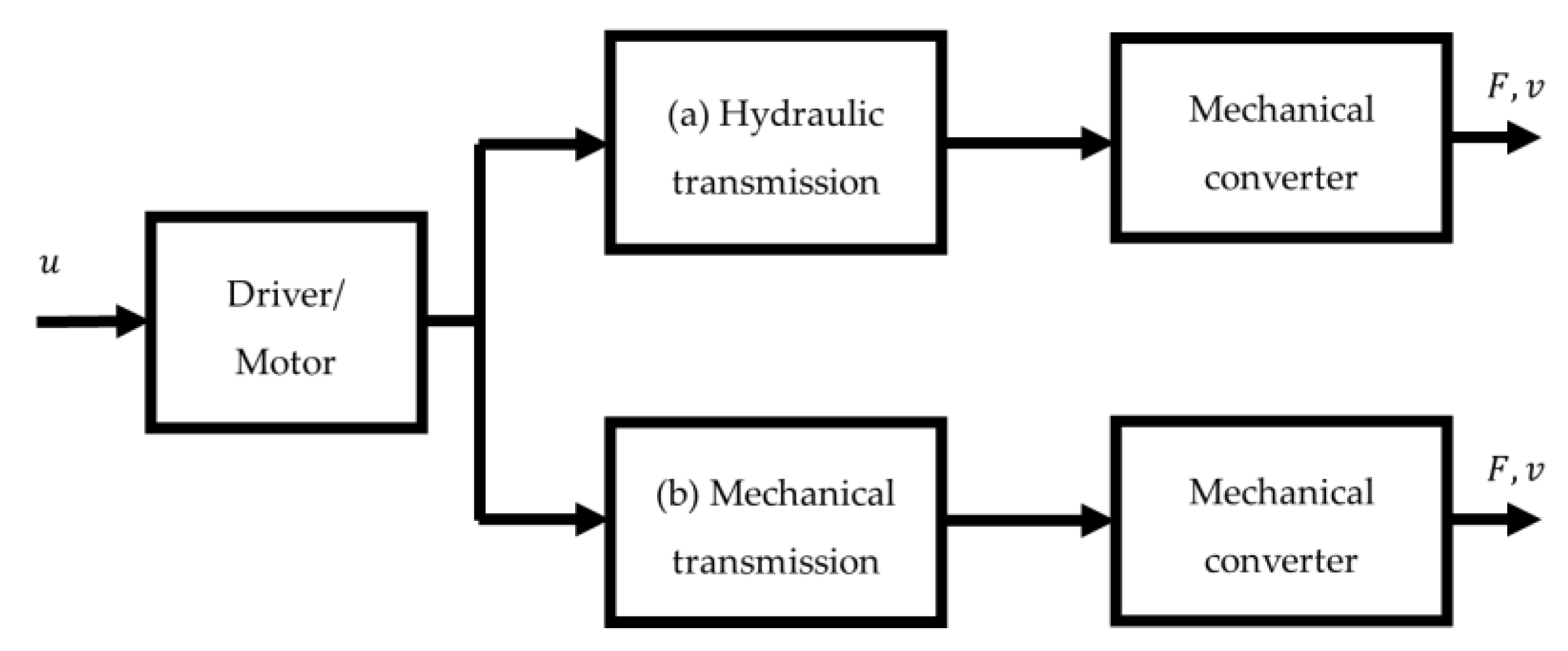
Figure 2.
Electrical DC motor complete block diagram.
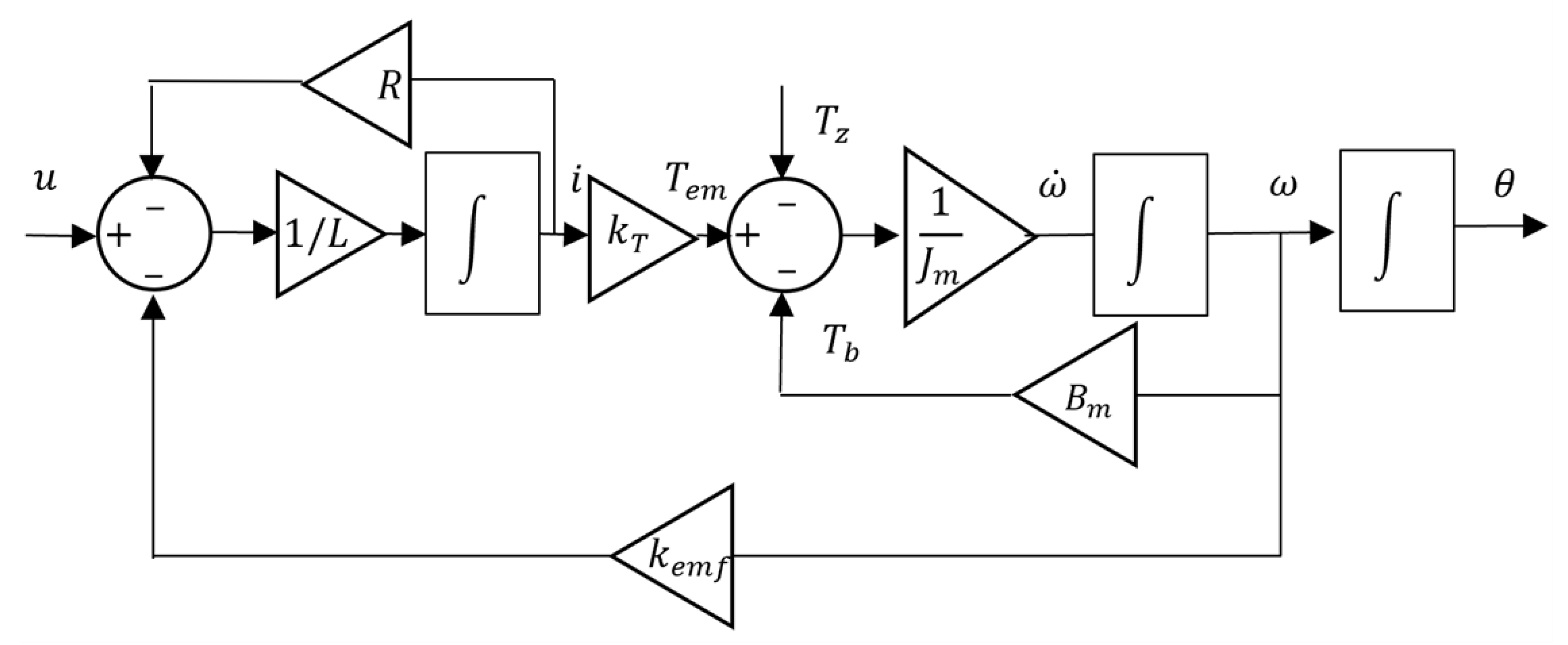
Figure 3.
Electrical motor simplified block diagram.

Figure 4.
Electrohydraulic circuit components.
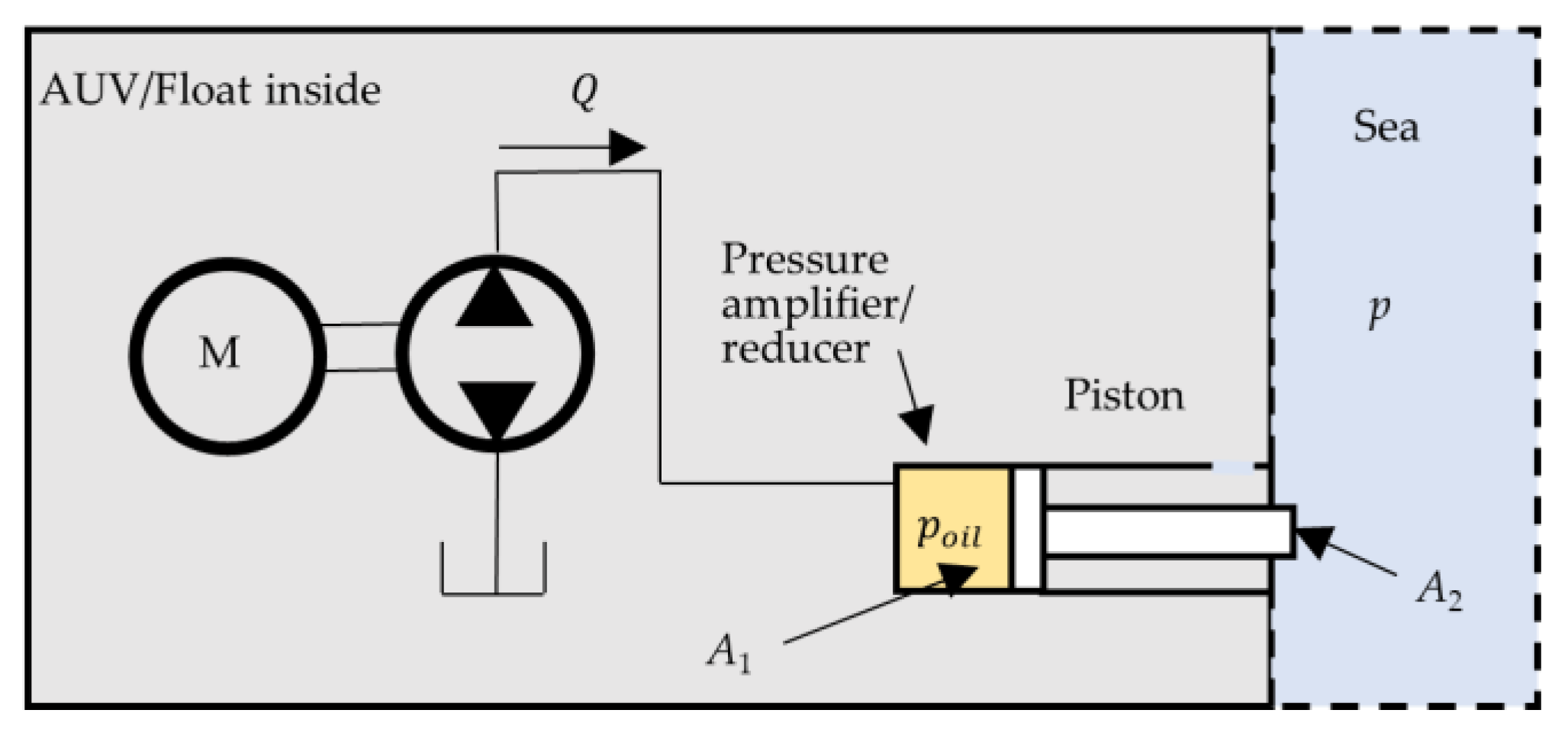
Figure 5.
Simplified block diagram of the electrohydraulic solution.
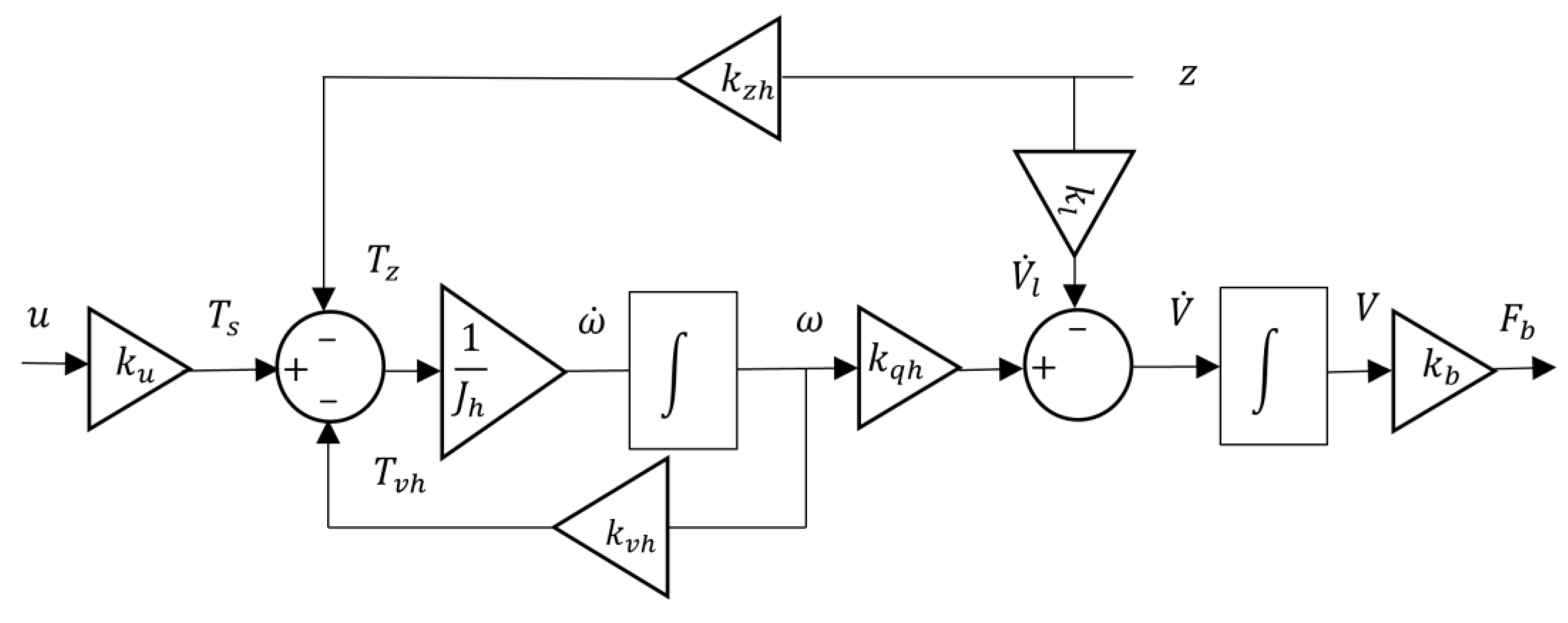
Figure 6.
Electromechanical solution components.

Figure 7.
Simplified block diagram of the electromechanical solution.

Figure 8.
Simplified unified block diagram for the actuation system of the VBS.
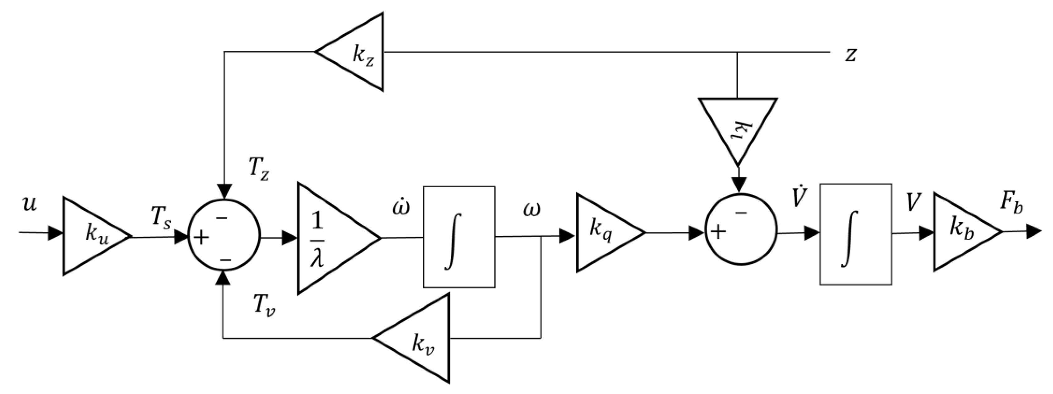
Figure 9.
Schematic of the forces acting on the VBS device.

Figure 10.
VBS overall device depth motion block diagram.
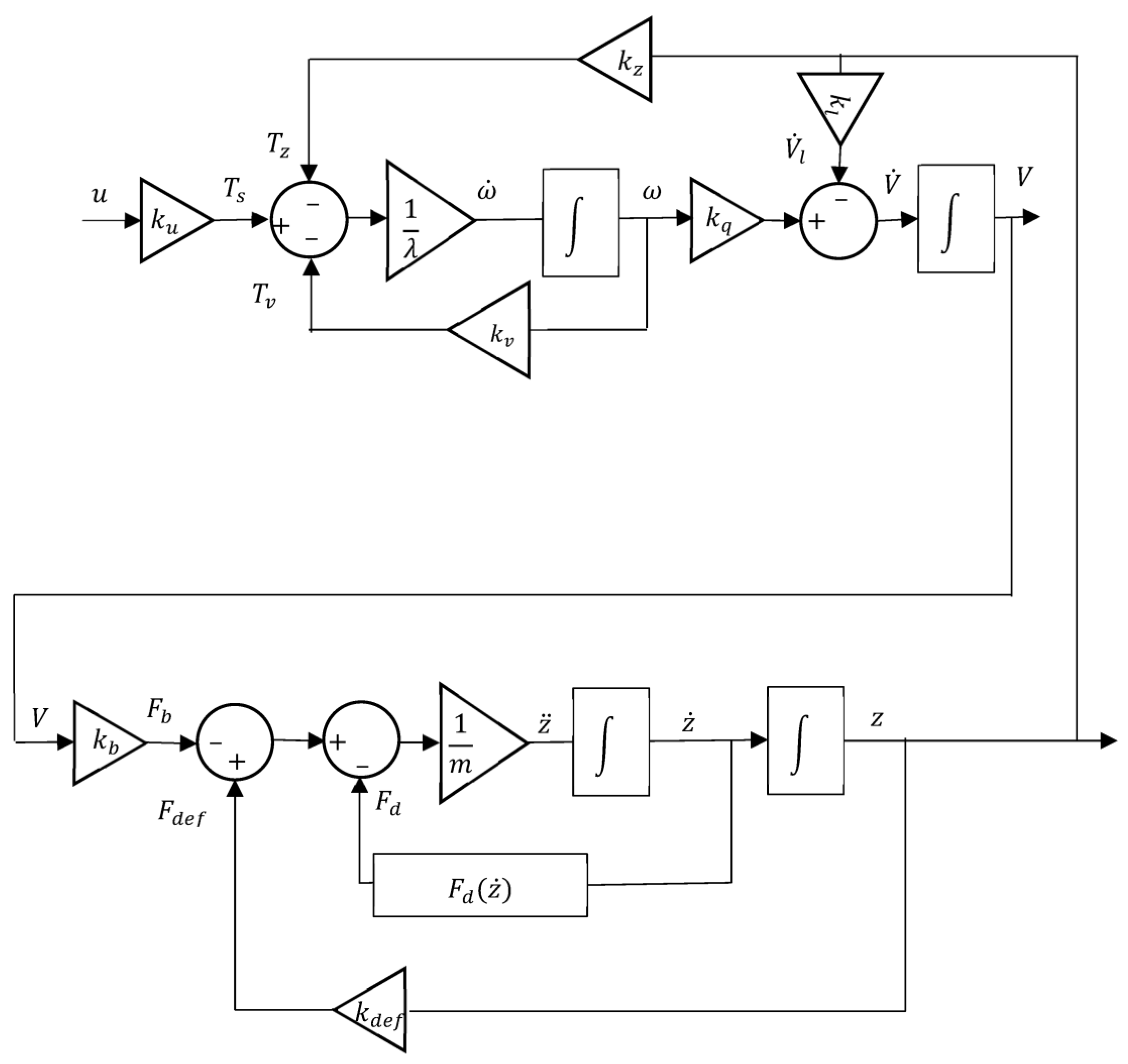
Figure 11.
Prototype used for model identification and control at the test pool.

Figure 12.
Evolution of depth (z) in time for the 4 steps of the experimental model identification procedure (a) to (d).
Figure 12.
Evolution of depth (z) in time for the 4 steps of the experimental model identification procedure (a) to (d).

Figure 13.
Depth velocity identification results: depth velocity evolution in time for different buoyancy changes.
Figure 13.
Depth velocity identification results: depth velocity evolution in time for different buoyancy changes.
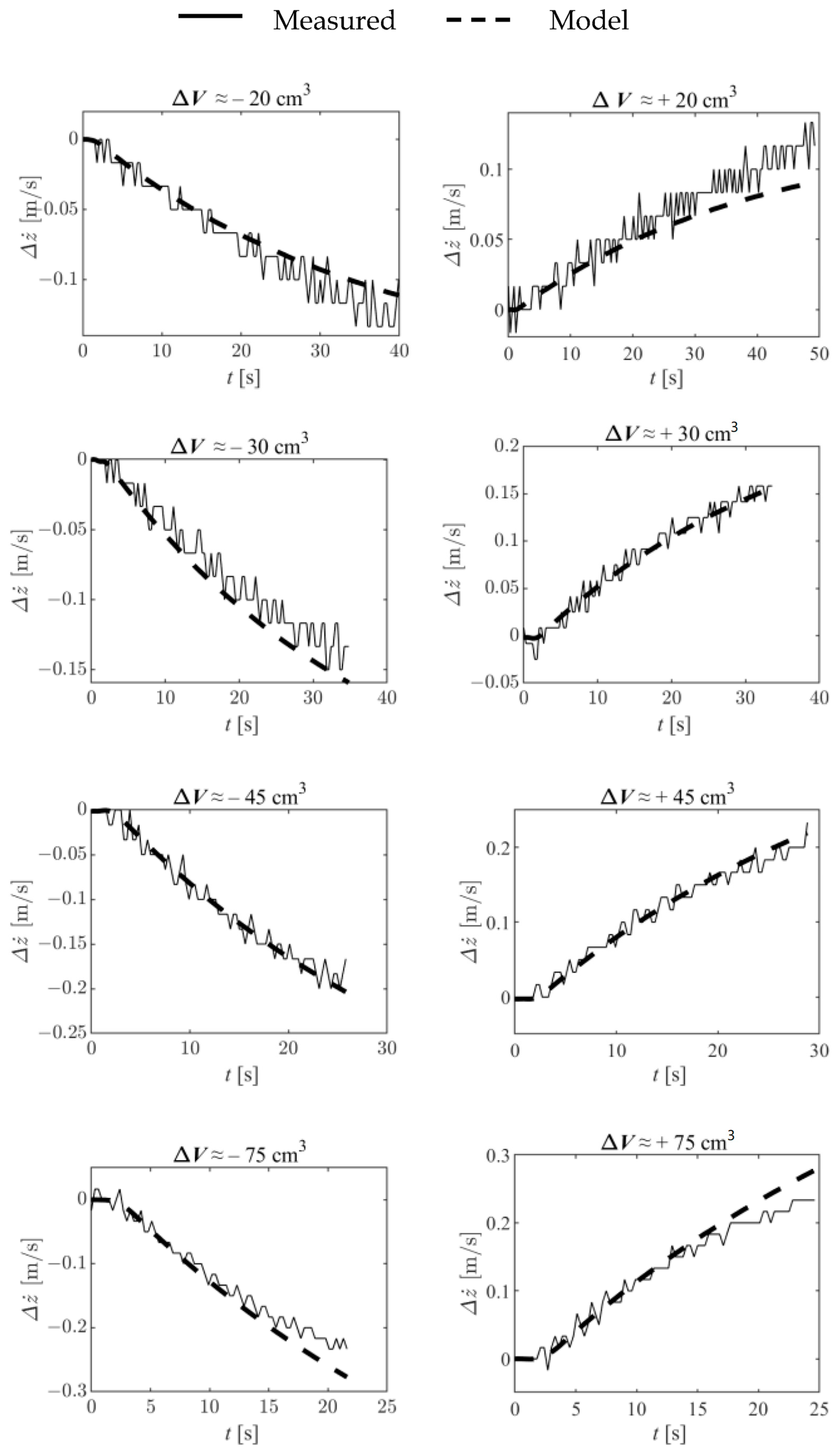
Figure 14.
Depth identification results: depth evolution in time for different buoyancy changes.

Figure 15.
Controller structure used in this work.
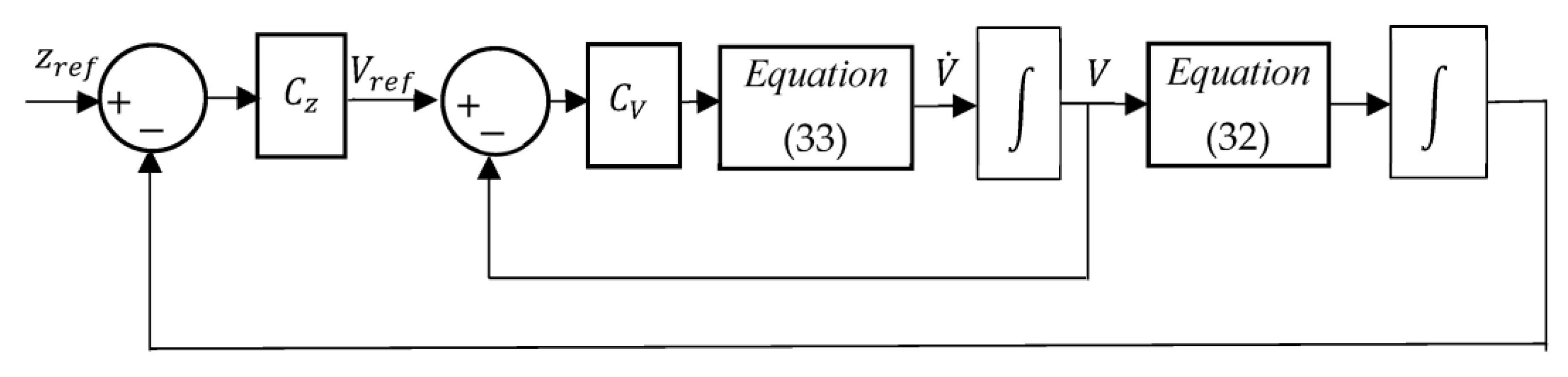
Figure 16.
Control results for depth steps of different amplitudes and directions.

Figure 17.
Control results for a longer step: (a) overall result; (b) zoom around target depth.

Table 1.
Constants and variables of Figure 8.
Table 1.
Constants and variables of Figure 8.
| Constant/Variable | (a) Electrohydraulic Solution | (b) Electromechanical Solution |
|---|---|---|
| Voltage applied to the motor | ||
| Stall torque of the motor | ||
| Torque caused on the motor with the increase in vehicle depth | ||
| Torque losses proportional to motor speed | ||
| Inertia of the motor plus the reflected inertia on the motor of the pump, moving oil, piston and added mass of the displaced water | Inertia of the motor plus the reflected inertia on the motor of mechanical reducer, spindle, piston and added mass of the displaced water | |
| Constant relating the control action and motor stall torque | ||
| Constant relating and the buoyancy force | ||
| Constant relating and | ||
| Volume of the piston | ||
| Motor velocity | ||
Table 2.
Model identification results for depth and depth velocity.
| Transfer Function | K (ms−1m−3) | T (s) |
|---|---|---|
| (26) | −7935.54 | 36.3 |
| (27) | −7634.95 | 35.7 |
Table 3.
Controller parameters used at the experimental trials.
| CV | CZ | |
|---|---|---|
| kp | 1002 (V × dm−3) | −0.1043 (dm3 × m−1) |
| ki | −7.486 × 10⁻⁴ (dm3 × s−1 × m−1) | |
| kd | −2.341 (dm3 × s × m−1) |
Disclaimer/Publisher’s Note: The statements, opinions and data contained in all publications are solely those of the individual author(s) and contributor(s) and not of MDPI and/or the editor(s). MDPI and/or the editor(s) disclaim responsibility for any injury to people or property resulting from any ideas, methods, instructions or products referred to in the content. |
© 2023 by the authors. Licensee MDPI, Basel, Switzerland. This article is an open access article distributed under the terms and conditions of the Creative Commons Attribution (CC BY) license (https://creativecommons.org/licenses/by/4.0/).
Share and Cite
MDPI and ACS Style
Falcão Carneiro, J.; Pinto, J.B.; Gomes de Almeida, F.; Cruz, N.A. Electrohydraulic and Electromechanical Buoyancy Change Device Unified Vertical Motion Model. Actuators 2023, 12, 380. https://doi.org/10.3390/act12100380
AMA Style
Falcão Carneiro J, Pinto JB, Gomes de Almeida F, Cruz NA. Electrohydraulic and Electromechanical Buoyancy Change Device Unified Vertical Motion Model. Actuators. 2023; 12(10):380. https://doi.org/10.3390/act12100380
Chicago/Turabian StyleFalcão Carneiro, João, João Bravo Pinto, Fernando Gomes de Almeida, and Nuno A. Cruz. 2023. "Electrohydraulic and Electromechanical Buoyancy Change Device Unified Vertical Motion Model" Actuators 12, no. 10: 380. https://doi.org/10.3390/act12100380
Note that from the first issue of 2016, this journal uses article numbers instead of page numbers. See further details here.