1. Introduction
The increasing need for integrating renewable energy sources, such as off-shore wind power and power harnessed from photovoltaic cells installed in deserts, has rekindled interest in high voltage direct current (HVDC) multi-terminal grids [
1]. China alone has plans to start around 30 HVDC transmission projects within the next 20 years [
2]. If realized, an HVDC system will be able to transport power from remote areas to consumers with very low losses. However, its feasibility relies entirely on the existence of an HVDC breaker that is able to interrupt fault currents within very short time intervals [
3]. To be able to interrupt fault currents promptly, an ultra-fast electromagnetic drive is needed to actuate the current carrying contacts by generating impulsive forces within hundreds of microseconds.
The mechanical part of a direct current (DC) circuit breaker consists of a contact system, an insulating medium, a pull rod, an ultra-fast drive and a control unit, as shown in
Figure 1. The contact system consists of an inlet (1), a pair of stationary and movable contacts (2a and 2b) and an outlet (3). A pull rod (4) connects the contact system to the drive. The drive consists of an armature (5) and opening and closing coils (6a and 6b), respectively. Spring-based bistables (7) are used to keep the armature in close contact with the opening drive coil or the closing coil. When a fault current emerges, the control unit is triggered so that the DC breaker’s drive can actuate the contacts promptly.
Figure 1.
A sketch of a DC breaker showing the current carrying contacts (2), the pull rod (4), the armature (5), the coils (6) and the bistables (7).
Figure 1.
A sketch of a DC breaker showing the current carrying contacts (2), the pull rod (4), the armature (5), the coils (6) and the bistables (7).
After separating the contacts of a DC breaker, an arc will be initiated. To extinguish it, one can use parallel branches with semiconductors or an oscillatory circuit to inject a high frequency current forcing a current zero crossing as the contacts are separating [
4]. The arc will then be extinguished at a current zero crossing. However, after contact separation, the breaker has to be able to withstand the voltage appearing across it. Otherwise, the arc might reignite, especially if the air gap separating both contacts is not sufficiently large.
The modeling of such a breaker is challenging, since it should be simulated with all of the necessary involved physics. As emphasized in [
5], the interaction of different physics can now be understood thanks to the available computational power. Some examples of recent nonlinear coupling between mechanical stress and electric fields can be found in [
6,
7]. In this paper, novel multi-physics hybrid and finite element method-based models are presented and compared.
2. Mechanical Challenges of an HVDC Breaker
The interest in DC breakers has increased over the past years [
2,
8,
9]. One of the main challenges of an HVDC breaker is to separate the current carrying contacts within a few hundreds of microseconds. Otherwise, due to the low impedance of a DC grid [
10], fault currents will rise quickly in magnitude and become harder to interrupt.
Similar linear actuators for high applications involving high accelerations are being investigated [
11]. For a circuit breaker, an example of a typical requirement could be to interrupt a short circuit current by accelerating the contacts from rest up to 25 m/s within 500
; corresponding to a peak acceleration in the order of 10,000 g. Assuming the mass of the breaker’s moving part to be around 5
, this would mean that the breaker will be subjected to an impulsive force of 500
after 250
. The combination of large forces and very short time scales poses a mechanical challenge, in particular when compared to a length scale in the order of meters.
In order to actuate the contact system this rapidly, an electromagnetic actuator that is capable of generating large impulsive forces is required. These actuators can be used in breakers and for other switching equipment, such as super conducting fault current limiters [
12]. Several actuation schemes can be developed to generate such forces [
13,
14,
15]. The actuator studied in this paper consists of a multi-turn flat spiral coil (
Figure 2), situated directly under a mushroom-shaped conductive armature (
Figure 3). Examples of similar actuation topologies applied to breakers can be found in [
16,
17,
18]. Discharging a capacitor bank comprising several series and parallel connected capacitors through the drive coil results in a large current surge that, in turn, generates a substantial magnetic field. The axial component of this time-varying magnetic field induces azimuthally-directed eddy currents in the armature. Then, the vector product of the phi-directional currents in the armature along with the radial component of the magnetic flux density results in an impulsive repulsive body force, later denoted by
.
Figure 2.
A picture showing a spirally-shaped coil and its contacts.
Figure 2.
A picture showing a spirally-shaped coil and its contacts.
Figure 3.
Mushroom-shaped conductive armature with threads on the stem’s extremity to screw in a pull rod.
Figure 3.
Mushroom-shaped conductive armature with threads on the stem’s extremity to screw in a pull rod.
This actuator cannot be directly connected to the metallic contacts. One strict requirement of an HVDC breaker is to actuate its contacts using an electrically-insulating material to prevent the fault currents to flow elsewhere. An insulating material that electrically isolates the contacts from the armature and yet allows the transmission of forces between them is required. This component is the above-mentioned pull rod ((4) in
Figure 1) and is usually made of composite materials or ceramics. The impulsive forces are generated in the armature and have to be first transmitted through the pull rod before they arrive at the desired location,
i.e., the metal contacts. The main part of the body forces are generated within the first few millimeters inside the armature, which is located directly on top of the coil. Depending on the system voltage level, the pull rod has to have a certain minimum length, denoted by
. The usual length of such pull rods is around 600
. The time it takes for a wave to propagate through the armature to the contacts denoted by
can be estimated using the velocity of waves (
) in a homogeneous isotropic medium with:
where
K,
G,
ρ,
E and
v are the bulk modulus, shear modulus, density of the medium, Young’s modulus and Poisson’s ratio.
In this study, a pull rod manufactured of fiberglass-reinforced epoxy (FR4) is investigated, since its properties are significantly superior to the traditional material used for such applications. It is electrically insulating and mechanically very strong with a Young’s modulus of 24 and a yield tensile stress exceeding 310 . It has a shear modulus of 11 and a density of 1850 kg/m. Furthermore, it can be machined in any desired shape and size, even if smoothness in shape should be striven for. If the travel time in the aluminum armature is neglected, then the time it takes for the wave to travel from one end of the pull rod to the other is around 160 , which is in the time scale of the HVDC breaker. This time may be even longer if a longer pull rod is used or the pull rod is manufactured of a material with a lower Young’s modulus. Therefore, in the following sections, different models are examined in order to study the influence of the pull rod mechanics on the force generation mechanism and the displacement of the armature.
3. Electromagnetic Modeling
The modeling of the actuator is divided into two parts, a circuit model and a finite element method (FEM) model, that are implemented in the software COMSOL Multiphysics (Version 4.3b, COMSOL AB, Stockholm, Sweden), as shown in
Figure 4 [
19]. An electrical source consisting of series and parallel-connected capacitors, a thyristor and cable leads connecting to a Thomson coil (TC) is modeled as a lumped circuit. On the other hand, the TC actuator that comprises a primary stationary coil and a mobile conductive armature is modeled using an FEM model. These two models are then coupled together and solved simultaneously.
Figure 4.
A SPICE circuit coupled to an FEM model for a Thomson coil. The coil and the armature are modeled using FEM, since the resistance and inductance of the coil and armature, and , are nonlinear and changing dynamically as the armature moves away. The capacitor, diode, thyristor and cables are modeled by lumped parameters.
To generate a large impulsive current, several parallel and series-connected capacitors are charged to a voltage denoted . The capacitor bank can be modeled as an effective capacitance in series with its effective resistance denoted by . As for the thyristor and the leads connecting the capacitor bank to the actuator, their impedance is lumped together and designated by and , respectively. A free wheeling diode is furthermore placed in parallel with the capacitor bank to prevent the build up of a negative voltage, since an electrolytic capacitor must be charged with only one polarity.
The finite element method is used to model the spiral coil and the armature solving the electromagnetic and mechanical equations at every time step. Concentric rectangles representing the width and depth of each coil conductor turn are drawn in a two-dimensional axi-symmetric geometry, avoiding the need to use 3D simulations and significantly reducing computation time. The voltage (
) across the spiral coil in the FEM model serves as the connecting point to the circuit model. The total coil voltages at the terminals of the circuit are distributed across the different coil turns by:
in such a way so as to ensure that the current (
) in each turn
n is identical to the currents in the other turns. Here,
is the externally-applied current density due to
, the voltage across each coil turn,
is the electrical conductivity,
is the current density and
s is the surface area of each conductor turn. The average radius of each turn is denoted by
.
The induced current density in the conductive mobile armature denoted by
moving with a relative velocity
is given by:
where
is the electric field and
is the magnetic flux density. As for the stationary base coil, its induced current density reduces to:
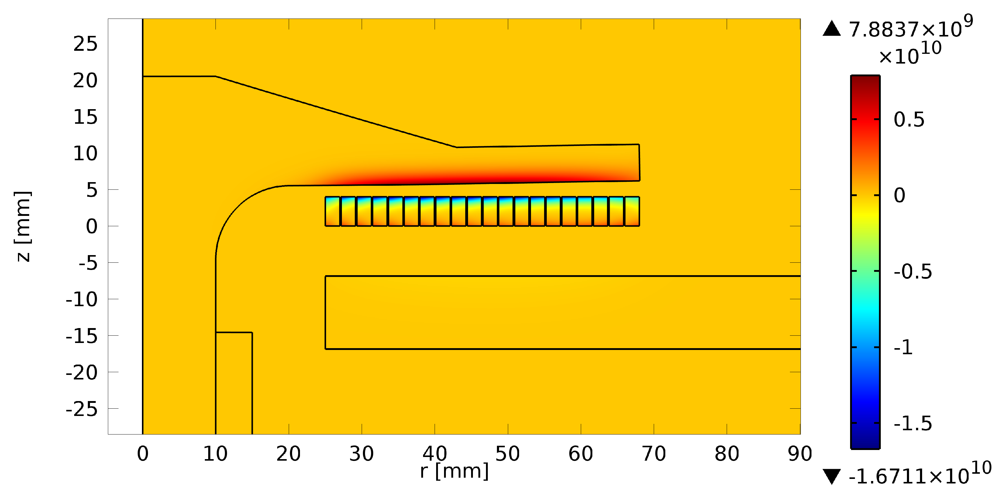
Figure 5.
The current density 100 after the discharge of the capacitor bank is distributed in only small portions of the geometry. Positive current densities appear in the top part of the coil conductors, while negative currents are induced in a piece of the armature situated directly above the coil.
The total current density in the coil and the armature can be expressed by:
respectively. An example of the current density distribution can be seen in
Figure 5. Based on Maxwell’s equations,
the magnetic equation for the primary coil,
, can be written as:
where
is the magnetic vector potential,
the magnetic field intensity,
the current density, ∇ the nabla operator,
μ the magnetic permeability and
the externally-applied current density. The magnetic equation for the mobile armature (
) is given by:
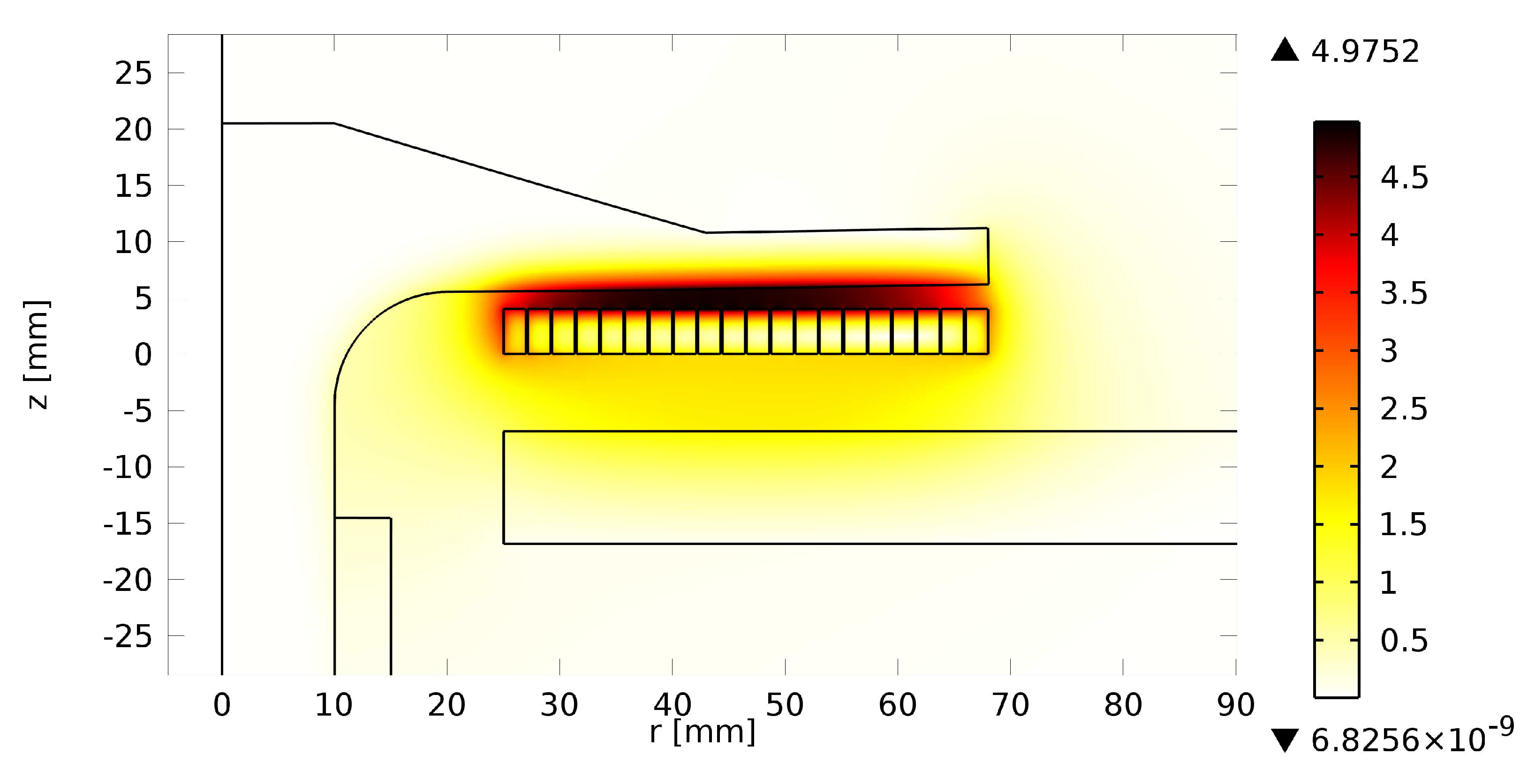
The magnetic flux density upon the discharge of the capacitor bank can be seen in
Figure 6. A current in the presence of a perpendicularly-oriented magnetic field results in a body force
, also know as a Lorentz force (see
Figure 7), where:
The force density is not homogeneously distributed and is generated only in the head of the mushroom, implying a high risk of deformations. In order to resolve these very small skin depths, triangular elements with a size around half a millimeter are used to mesh the zone where the force is generated. Although increasing the memory demands, second order elements are used to catch the gradients.
Figure 6.
The magnetic flux density 100 after the discharge of the capacitor bank reaches 5 and is highest in the air gap separating the coil and the armature.
Figure 6.
The magnetic flux density 100 after the discharge of the capacitor bank reaches 5 and is highest in the air gap separating the coil and the armature.
Figure 7.
Force density 100 after the discharge of the capacitor bank. The coil is subjected to compressive forces, while the armature is subjected to an axially-directed body force that is mostly concentrated in the first few millimeters closest to the coil.
Figure 7.
Force density 100 after the discharge of the capacitor bank. The coil is subjected to compressive forces, while the armature is subjected to an axially-directed body force that is mostly concentrated in the first few millimeters closest to the coil.
This transient may last for several milliseconds. In this model, a variable time step is implemented using very small time steps only when needed to ensure convergence. The smallest time step is around 50 and is only required when the voltage of the capacitor bank reaches zero, activating the highly nonlinear model of the free wheeling diode. Otherwise, a time step of around 10 is enough to have a good resolution.
The computed displacement is used to implement a moving mesh, which is vital to account for the movement of the armature. As the armature repels, skin depth and inductance increase. Therefore, the net resistance of the material decreases, since a larger cross-section of the conductor is utilized. The technique used is based on the arbitrary Lagrangian–Euler method, whereby the mesh is progressively stretched until a quality limit is violated. The mesh quality or a specified element stretching factor serve as criteria to stop the simulation, re-mesh and interpolate the results from the previous mesh to the newly-generated mesh.
5. Model Validation by Experiments
One aim of the following experiments was to primarily study the influence of bending on the performance of the drive and, secondly, to see its effect on the current pulse. Another aim was to validate the full multi-physics model (Model 1) and the infinitely stiff model (Model 4) using two differently-dimensioned armatures.
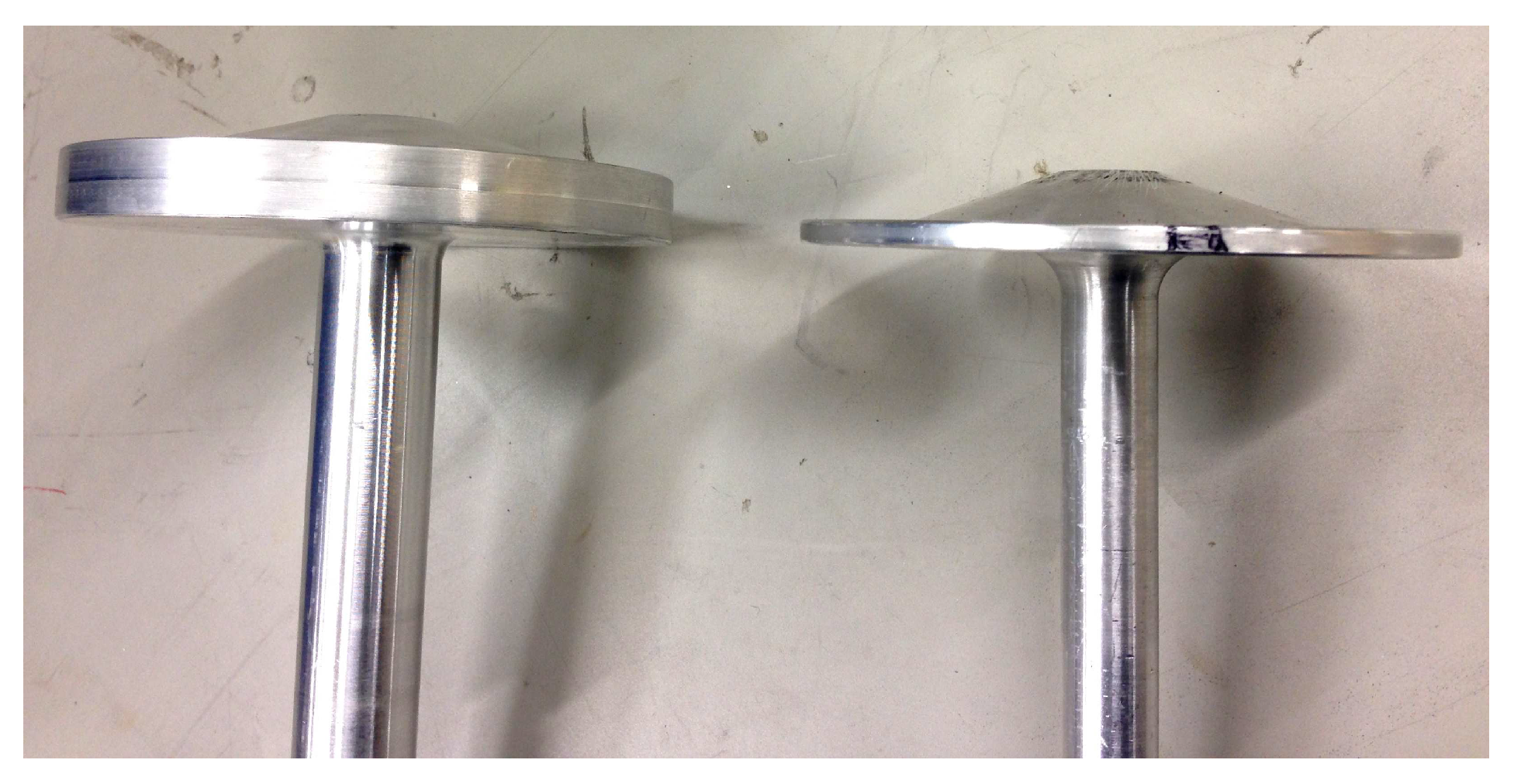
To verify the simulation models, an experimental setup was built with two armature variants shown in
Figure 9. The first armature is slim and is prone to bending when subjected to an impulsive force, while the other is larger and thereby more robust and rigid. Both armatures were however designed to withstand the maximum stresses.
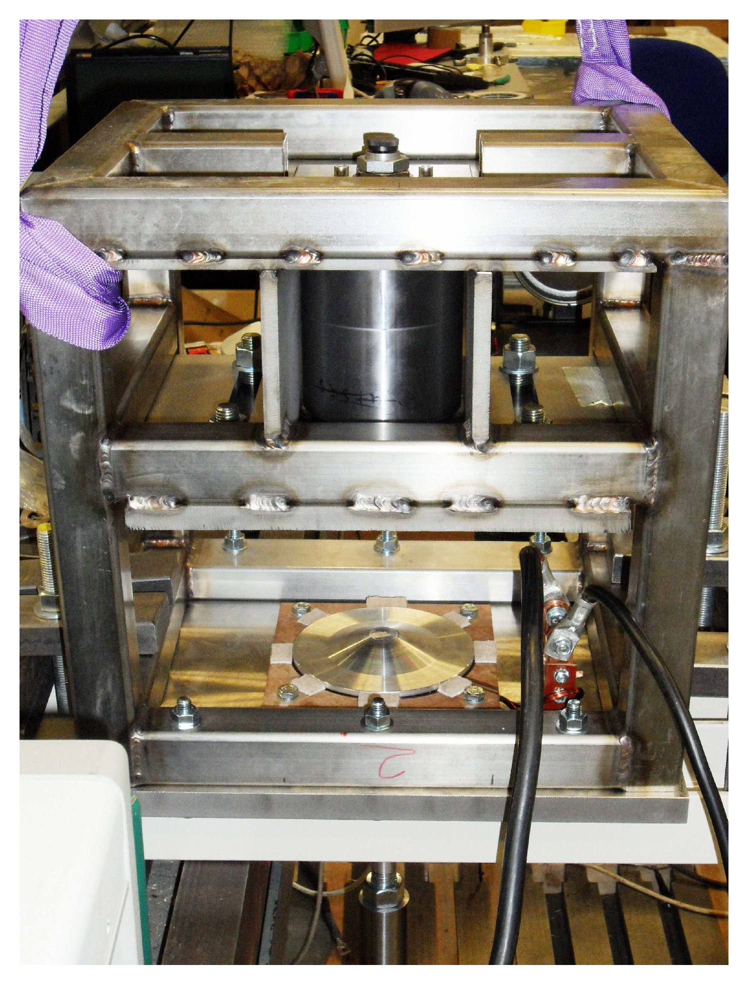
The experimental setup can be seen in
Figure 10. The mushroom-shaped armature is lying on top of a flat spiral coil, which is connected to a capacitor bank. A large steel structure was used to avoid vibrations and clamp down the setup firmly to a very heavy steel table. At this stage, the pull rod is omitted, and the masses are directly attached to the armature. Two steel masses, weighing 3.6
and 1.5
, were firmly attached to the slim and large armatures, respectively. Two capacitor banks with capacitances of 33
and 11
capable of being charged to 500
and 900
were used for the slim and large armatures, respectively.
Figure 9.
A picture showing the slim and large mushroom-shaped armatures. Although both are designed to withstand the mechanical stresses, one is flexible and prone to bending, while the other is more robust and stiffer.
Figure 9.
A picture showing the slim and large mushroom-shaped armatures. Although both are designed to withstand the mechanical stresses, one is flexible and prone to bending, while the other is more robust and stiffer.
Figure 10.
A picture showing the experimental setup. The slim mushroom armature is sitting on a flat spiral coil that is connected with large cables to a capacitor bank. It is mounted with a 3.6 steel mass.
Figure 10.
A picture showing the experimental setup. The slim mushroom armature is sitting on a flat spiral coil that is connected with large cables to a capacitor bank. It is mounted with a 3.6 steel mass.
A Pearson probe was used to measure the current pulses. Initially, accelerometers were used to measure the acceleration of the armature. However, since high accelerations and collisions are involved in these experiments, the accelerometers break quickly. Instead, a high speed camera with frame rates of 100,000 fps was used to film the armatures. Afterwards, the images were calibrated and tracked to determine the velocity and the bending of the armature.
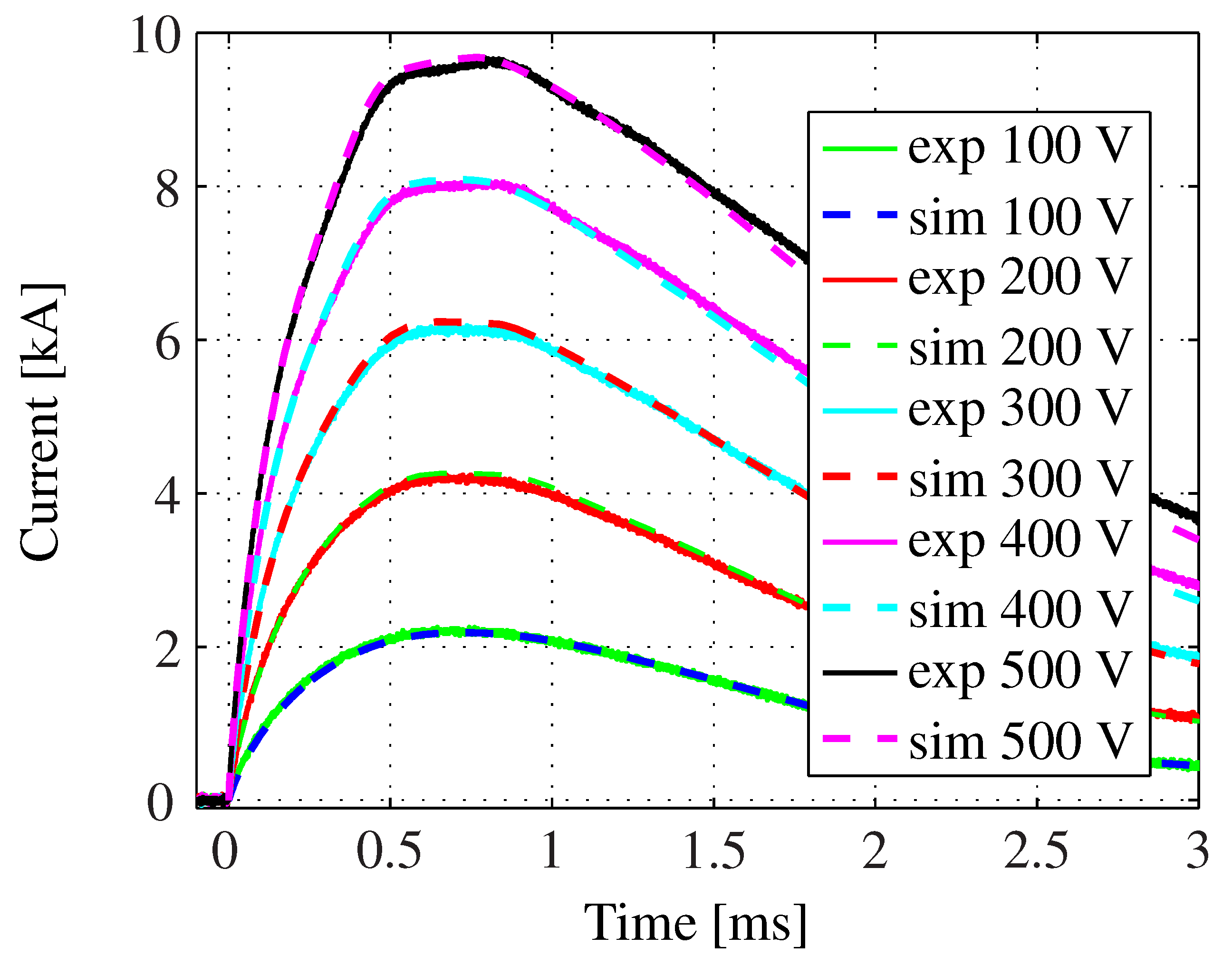
The simulated and measured current pulses for the slim armature are shown in
Figure 11. Since bending is expected, Model 1 is used. At low voltages, the current pulse has only one peak at 750
and looks smooth. However, when the charging voltage, and thereby the energy, was increased, the current pulse became distorted. A clear distinct camel hump current pulse can be seen following a 500
discharge. Two peaks appear, one at 550
and one at 850
. The second current peak is even higher than the first one.
Figure 11.
A picture showing the measured currents (solid lines) and the simulated currents (dashed lines) of the slim armature for increasing charging voltages in steps of 100 V.
Figure 11.
A picture showing the measured currents (solid lines) and the simulated currents (dashed lines) of the slim armature for increasing charging voltages in steps of 100 V.
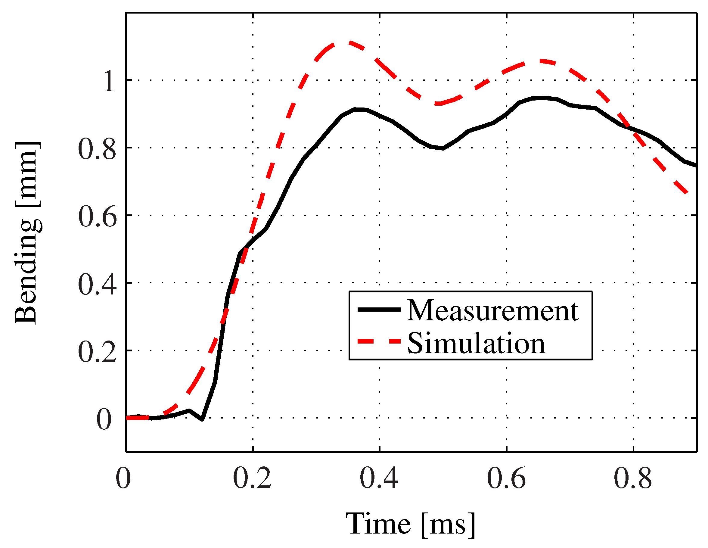
To explain the camel hump behavior of the current pulse, the bending of the mushroom armature was measured and compared to simulations; see
Figure 12. The camera was focused on the head of the mushroom only. The wing of the armature, as indicated by pt A in
Figure 13, and the top flat part of the armature were tracked. The difference between these two points is defined by bending. The simulations were able to predict the experimental results with a good degree of accuracy. Although there are small differences in absolute values, the trend of the bending is captured. Two sources of error are due to filming the mushroom with an angle and the loss of focus after 800
. This trend can be seen in the current pulse. The second current peak, at 850
, is due to the wing of the armature bending back when the internal elastic forces exceeded the repulsive electromagnetic force. The mutual coupling is increased with smaller air gaps. The overall inductance seen by the system becomes smaller, causing the current to rise towards a second peak.
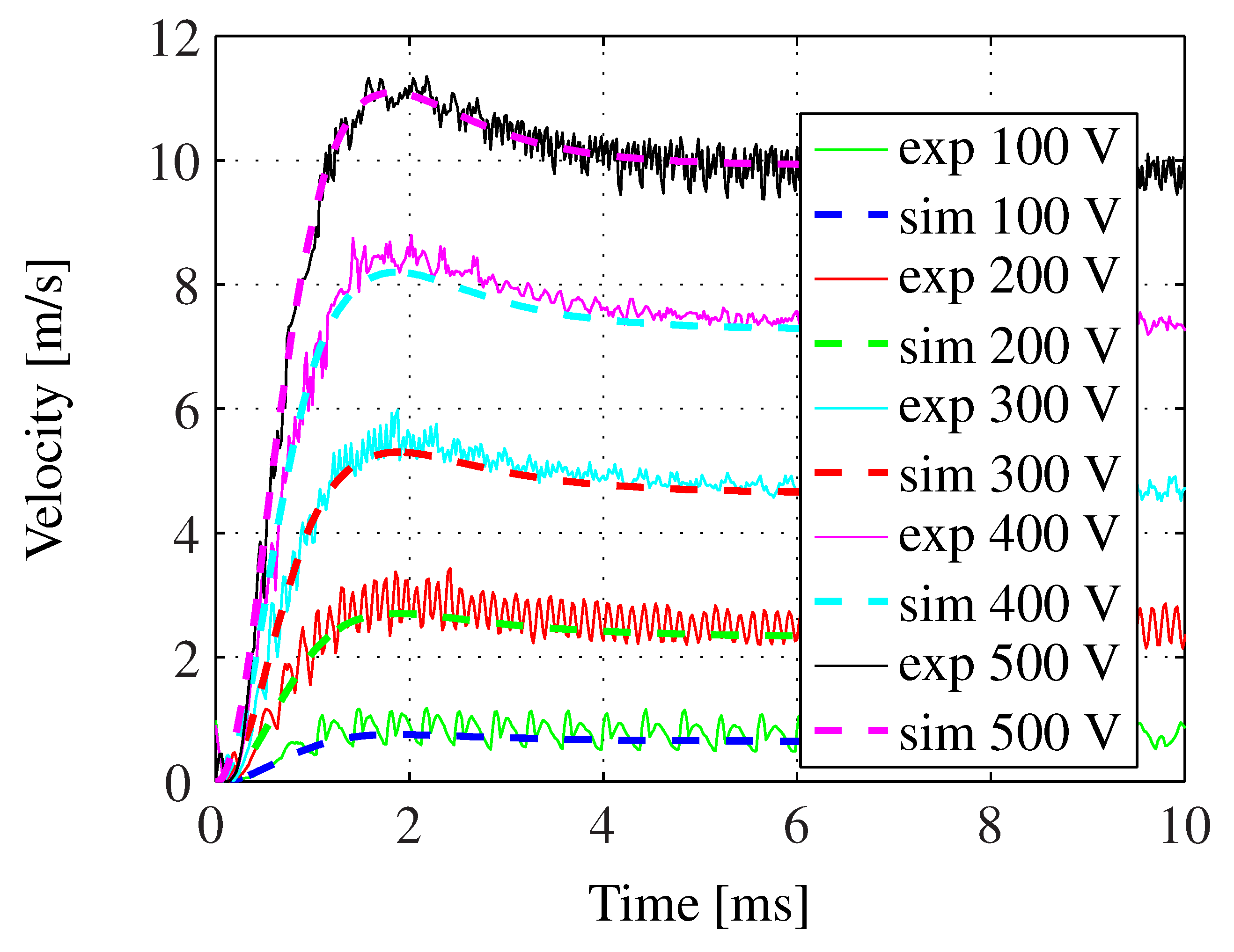
The measured and simulated velocities of the slim armature for different charging voltages are shown in
Figure 14. It can be seen that the model predicts the behavior of the armature well.
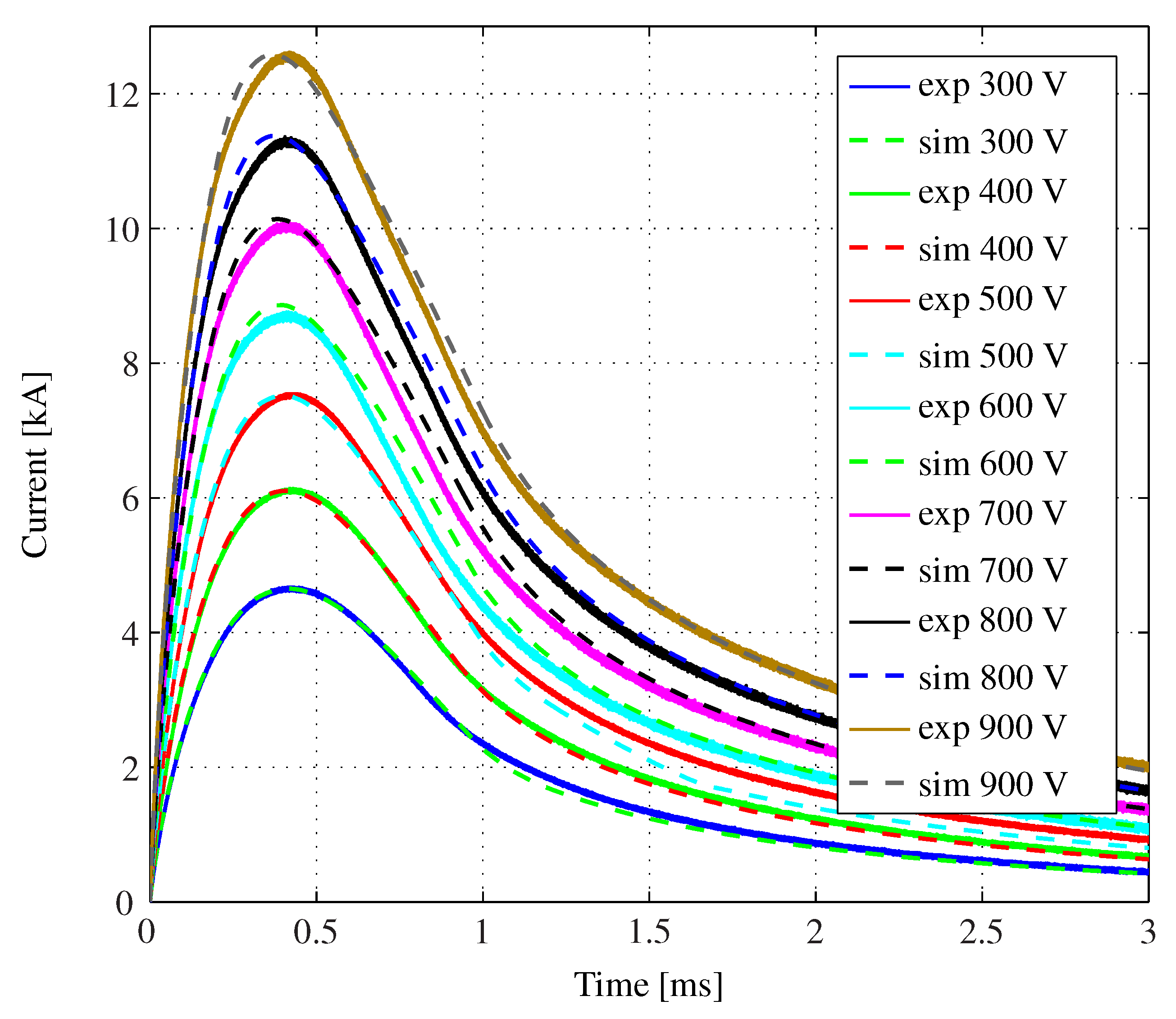
The simulated and measured current pulses for the large armature are shown in
Figure 15. In this case, since the armature was designed to minimize bending, the rigid simulation model (Model 4) was used. For low voltages, the measured and simulated current pulses are almost identical. However, for larger voltages, the simulated currents peak at an earlier time in comparison with the measured current pulses. Evidently, even such a bulky armature will bend and elongate when subjected to impulsive forces of this magnitude. In reality, any kind of elasticity will result in a larger system inductance, delaying the peak of the current pulse. Furthermore, the current pulses at all charging voltages have only one peak. Unlike the previous case, this indicates that very little bending exists.
Figure 12.
Comparison of the measured and simulated bending of the mushroom armature upon the discharge of a capacitor bank charged with 500 V. The bending cannot be measured for longer time scales, since the picture loses focus with large displacements, rendering the tracking unreliable.
Figure 12.
Comparison of the measured and simulated bending of the mushroom armature upon the discharge of a capacitor bank charged with 500 V. The bending cannot be measured for longer time scales, since the picture loses focus with large displacements, rendering the tracking unreliable.
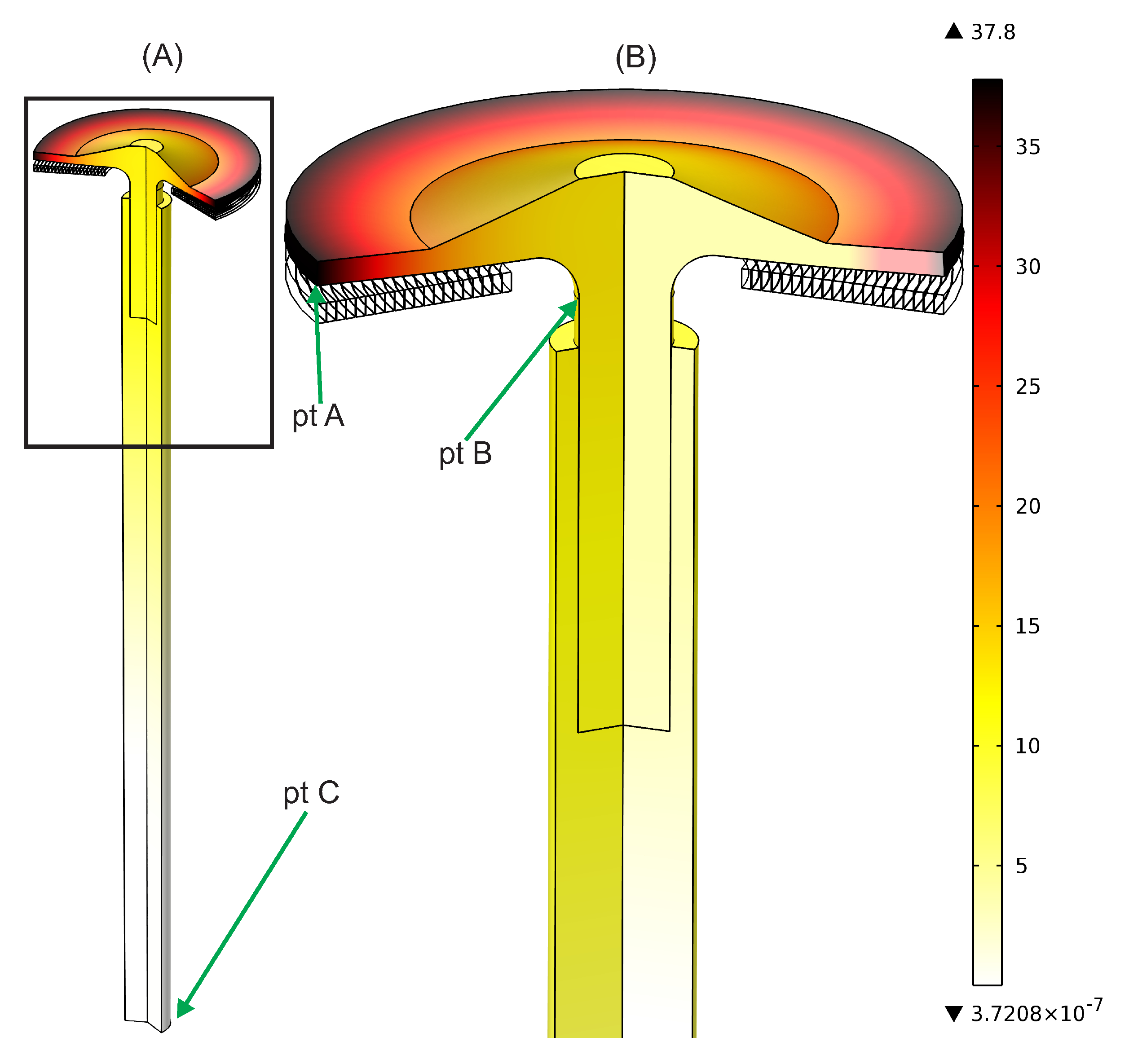
Figure 13.
A 3D picture showing the velocity profile of the system in (m/s) after 150 . (B) Zoom in of the entire actuator shown in (A). The armature that is situated directly on top of the coil is threaded into a pull rod and attached firmly. Point A is located at the outermost extremity of the mushroom armature. Point B is located at the top of the stem of the armature, i.e., just below the rounded corner joining the head of the mushroom to its stem. Point C is located on the bottom of the pull rod, i.e., where the copper contacts are attached.
Figure 14.
A picture showing the measured velocities (solid lines) and the simulated velocities (dashed lines) of the slim armature for increasing charging voltages in steps of 100 V.
Figure 14.
A picture showing the measured velocities (solid lines) and the simulated velocities (dashed lines) of the slim armature for increasing charging voltages in steps of 100 V.
Figure 15.
A picture showing the measured currents (solid lines) and the simulated currents (dashed lines) of the large armature for increasing charging voltages in steps of 100 V.
Figure 15.
A picture showing the measured currents (solid lines) and the simulated currents (dashed lines) of the large armature for increasing charging voltages in steps of 100 V.
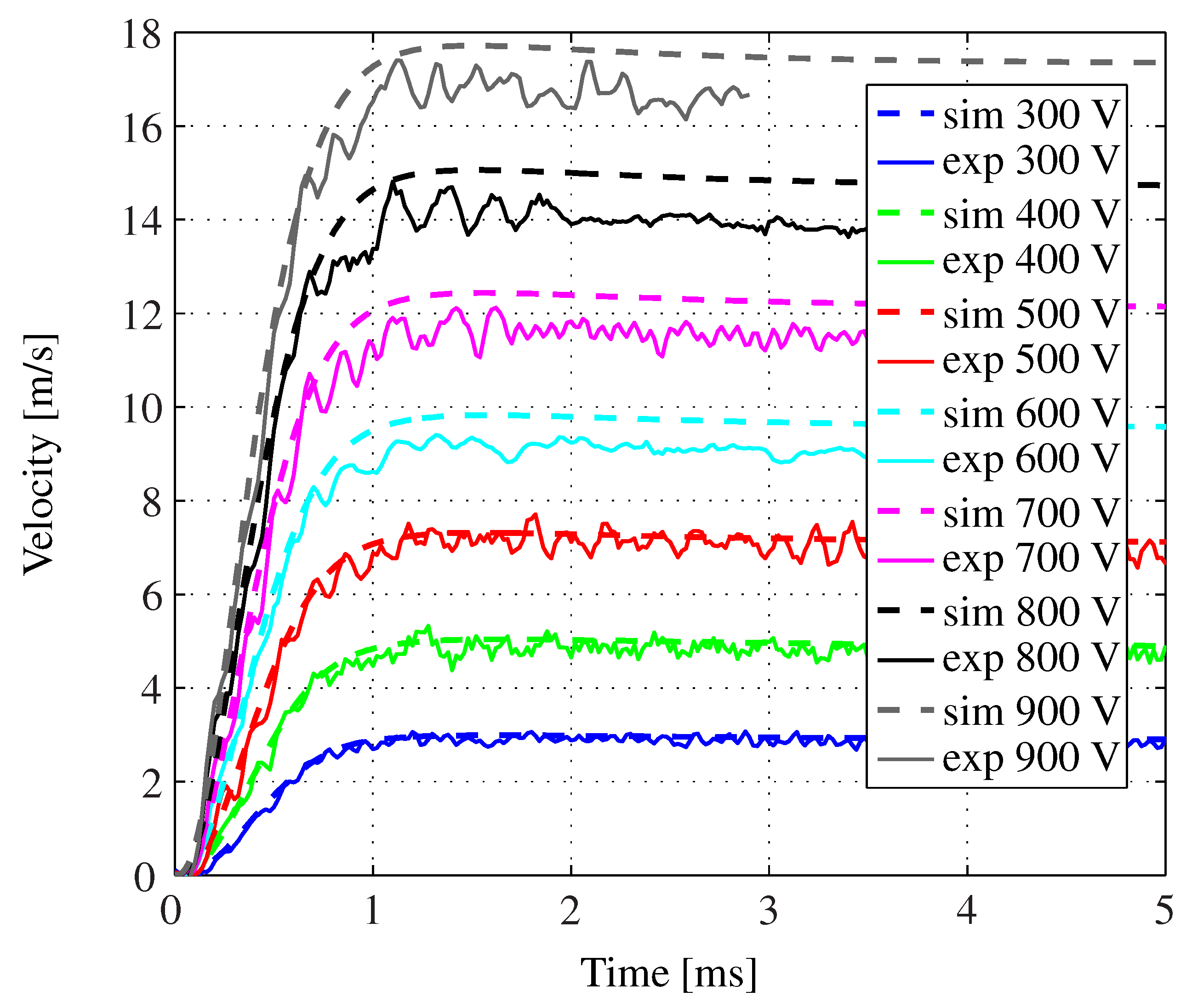
The simulated and measured armature velocities for the large armature are shown in
Figure 16. For such an armature, Model 4 can definitely be used to simulate the velocity of the armature with high accuracy. A small discrepancy exists at high voltages due to the inevitable presence of small deformations.
Figure 16.
A picture showing the measured velocities (solid lines) and the simulated velocities (dashed lines) of the large armature for increasing charging voltages in steps of 100 V. The simulation error increases with increasing impulsive forces, since even the large armature is elastic and will therefore bend eventually.
6. Results and Discussion
Following the model validations in the previous section, a pull rod was added, and different cases were simulated. From Model 1, the velocity distribution in the armature and the pull rod 150
after the discharge of a capacitor bank can be seen in
Figure 13. The extremities of the mushroom attain velocities up to 38 m/s, while the velocity of the load attached at the bottom of the pull rod is still zero. This large velocity gradient was expected and was estimated initially from Equation (
1).
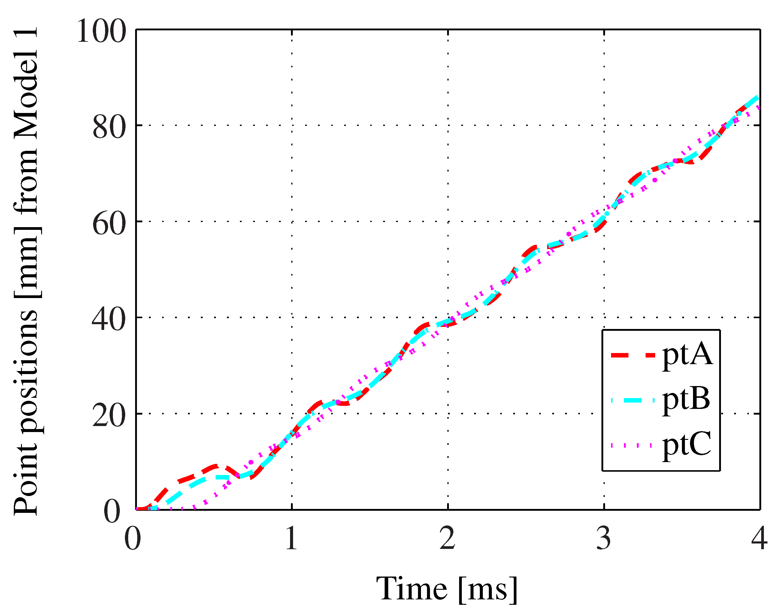
Figure 17 shows the displacements of different points of the armature-contact system as computed by Model 1. The difference between the displacements of Points A and B show that bending occurs in the range of several millimeters, while the difference between Points B and C show that the armature and the pull rod elongate prior to any movement of the actual load. It can be seen that 300
after discharge, Point A of the armature is displaced by 6
, whereas the contacts are still stationary.
Figure 17.
The displacements of three different points characterizing the dynamic motion of the breaker. The bending of the head of the mushroom can be computed by subtracting the axial displacement of ptB from that of pt A. Similarly, the elongation of the pull rod and the stem of the mushroom armature can be computed by subtracting the displacement of pt C from that of pt B.
The generated current impulse in the coil is highly sensitive to the stiffness of the system, but also to the chosen model. The repulsion of the head of the mushroom causes a premature air gap, which decreases the mutual inductance between the coil and the armature. This leads to a larger system inductance, limiting the sharp increase of the current pulse. This effect can be seen in
Figure 18, when comparing the current pulses computed from Models 1 and 4. The time derivative of the current pulse decreases, leading to a shift in the current peak in time and a decrease in magnitude. If the pull rod is assumed to be infinitely stiff, then only bending and elongation of the armature are present, and the effect on the current pulse is slightly mitigated. A current peak, slightly delayed in time and lower in magnitude, occurs in Model 3. As for Models 1 and 2, they give similar current pulses. Thus, a system that is subjected to both bending and elongation yields a lower current pulse and, thereby, a considerable decrease in efficiency.
The generated force impulse is inversely proportional to the square of the length of the air gap separating the top of the coil from the bottom of the armature. As
Figure 19 shows, a stiff system gives a significantly larger peak force than a system subjected to bending and elongation. Model 4 gives the highest peak force, followed by Model 3. Models 1 and 2 give similar peak force values, but the generated force impulses differ slightly in shape.
The displacements of the contacts
versus time is given in
Figure 20. As explained above, Models 1 and 2 give similar displacements, but oscillate out of phase. Therefore, after inspecting the current impulses, the force impulses and the displacements using Model 1 as a benchmark, it can be deduced that Model 2 gives similar results and can predict the behavior of the contacts with good accuracy. However, Models 3 and 4 are not good enough, since they overestimate the generated electromagnetic forces. Model 4 overestimated the peak force by almost 100%. Model 3 can be used if a stiff pull rod is used, while Model 4 can be used if both the armature and the pull rod are designed not to bend and elongate. They cannot, however, be considered as generally reliable for the present simulations with demands for accurate deformation and short time scales.
Figure 18.
The arising current pulse in the four models following the discharge of the capacitor bank in the spirally-shaped coil.
Figure 18.
The arising current pulse in the four models following the discharge of the capacitor bank in the spirally-shaped coil.
Figure 19.
The arising force impulse in the four models following the discharge of the capacitor bank in the spirally-shaped coil.
Figure 19.
The arising force impulse in the four models following the discharge of the capacitor bank in the spirally-shaped coil.
Figure 20.
The displacement of the load with respect to each model.
Figure 20.
The displacement of the load with respect to each model.
Investigation of Using Models with Finer Segmentations
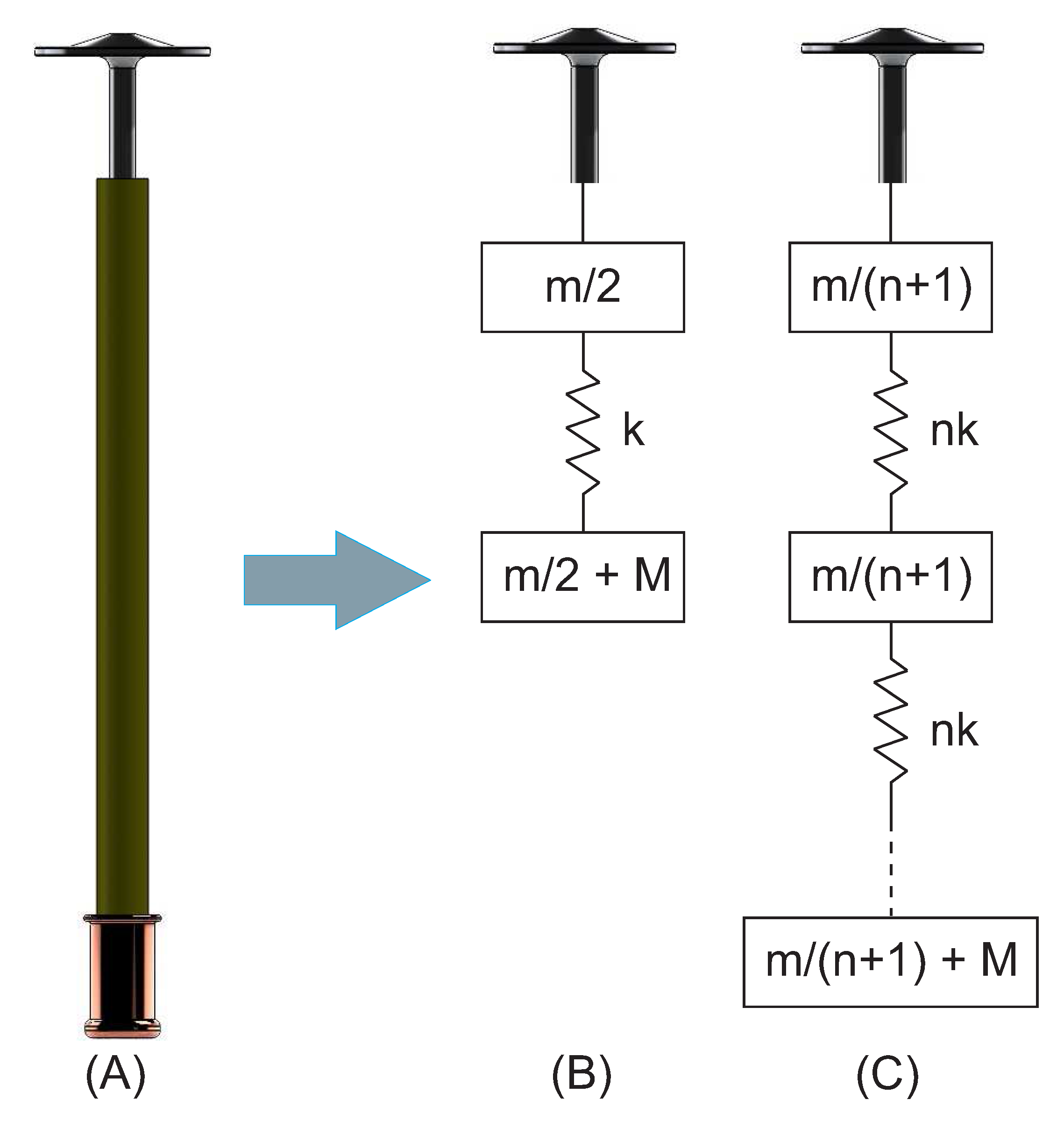
Since Model 2 gave excellent results, three more models were developed, denoted as Models 5, 6, and 7. These are hybrid models similar to Model 2, but give a more refined modeling of the pull rod by dividing it into 2, 3 and 10 spring segments; see
Figure 8.
Figure 21 shows a representative main displacement of the contact from all models. It can be inferred that although the complexity of the system is increased with finer segmentations of the pull rod, this does not necessarily lead to better results. The results obtained from these extra models are, however, consistently closer to those from the accurate Model 1 than the results from Models 3 and 4.
Figure 21.
The displacement of the load with respect to each model. Model 2: first order hybrid model. Model 5: second order hybrid model. Model 6: third order hybrid model. Model 7: Tenth order hybrid model.
Figure 21.
The displacement of the load with respect to each model. Model 2: first order hybrid model. Model 5: second order hybrid model. Model 6: third order hybrid model. Model 7: Tenth order hybrid model.
7. Conclusions
In an HVDC system, a breaker should be able to interrupt fault currents before they reach large values. It has been shown that the entire system, including the armature, the pull rod and the contacts, has to be taken into consideration in the design process, since this has a large influence on the magnitude of the generated force impulse and the efficiency of the actuator. From an electrical point of view, fast contact separation in the order of a couple of millimeters is crucial. With the developed multi-physics and hybrid models, the highly transient and complex magneto-mechanical interaction can be captured and modeled. The modeling can be used to build a high-end HVDC breaker with the desired specifications.
A system that is infinitely stiff will have a significantly higher efficiency, since it will fully utilize the potential of the electromagnetic drive. Deformations cause the armature to repel prematurely, causing larger air gaps and thereby limiting the build up of the force impulse before it attains its full potential. Optimizing the armature alone without consideration of the pull rod and the contacts is useless if the pull rod is allowed to elongate excessively. The breaker should be designed in such a way that deformations should be limited to fractions of a millimeter.
The developed hybrid first order multi-physics model has shown promising results and can predict the performance of the breaker with sufficient accuracy. Compared to the full multi-physics simulation model, it requires significantly less computational power and will solve the problem in a shorter period of time. Furthermore, the model does not need to be re-meshed as often, since only the armature has to be fully modeled. The increasing complexity obtained by subdividing the pull rod into several segments is shown to be of limited importance for the accuracy of the simulations. This developed model can be used to design the shape and the energizing source of the actuator to boost its efficiency. One limitation of the simplified hybrid model is that it can only be used if the push/pull rod has a linear stress-strain relationship.
Future work will be dedicated to the development of an optimization model to minimize the mass of the pull rod, while constraining its internal stresses and its elongation, to reduce the degradation of the force impulse. Furthermore, the effect of adding damping in parallel to the spring in the hybrid model will be investigated.


