What Is an Artificial Muscle? A Systemic Approach.

Abstract

Artificial muscles define a large category of actuators we propose to analyze in a systemic framework by considering any artificial muscle as an open-loop stable system for any output which represents an artificial muscle dimension resulting from its “contraction”, understood in a broad meaning. This approach makes it possible to distinguish the artificial muscle from other actuators and to specify an original model for a linear artificial muscle, according to the theory of linear systems. Such a linear artificial muscle concept exhibits a constant stiffness independent on its control value. It is shown that a biomimetic actuator, made of two antagonist artificial muscles, requires that artificial muscle static characteristic, even in its most simplified form, is non-linear in the meaning of systems theory, to make possible the control of both actuator position and stiffness. However, we also attempt to show that a linear viscous damping can be a practical way for the dynamic behavior of the artificial muscle to be in relatively good accordance with the so-called Hill curve, interpreted as the dynamic characteristic linking the maximum contraction velocity of the artificial muscle to varying loads lifted against gravity.

1. Introduction

Artificial muscle is a kind of actuator generally defined by analogy with the skeletal muscle. Like the natural muscle, any artificial muscle is characterized by its ability to contract in response to a chemical or physical stimulus. While contraction in skeletal muscle is essentially understood as a straight contraction, the term contraction applied to artificial muscle is used in a broader meaning: this can be the straight contraction of a more or less complex structure in the case of fluidic artificial muscles with a sheath, or the straight contraction of thin string in the case of shape memory materials, like filaments of Nitinol, but also the bending of strings, like in the case of some ionic electronic active polymers or, even, the extension of thin plates, as in the case of dielectric elastomers. In a general way any material, or device, whose shape can change in response to a stimulus can potentially be a candidate to the label “artificial muscle”. This very large, broad definition of the artificial muscle notion can explain the difficulty to synthetic reviews of all kinds of artificial muscles [1,2,3,4,5]. The aim of this paper does not deal with this complex problem of looking for the best strategy for classifying the various types of artificial muscles but consists to attempt to propose a global definition of the notion of artificial muscle. Our approach is based on the evident fact that any artificial muscle generates a force or torque in response to a stimulus whose consequence is a “contraction”—understood in a broad manner—to which can be associated a privileged variable dimension. One major difficulty, however, to define the peculiar actuation nature of the artificial muscle, in comparison with other actuators, is the actual lack of what could be called a general theory of actuators. Actuators can, indeed, be classified according to their energy conversion mode [6] or by means of selected criteria [7]. The skeletal muscle itself, as a “living actuator”, can be characterized by a list of performances concerning, for example, its density, stress, stiffness, strain, strain rate, power, energy, number of life cycles, and efficiency and the values corresponding to these criteria can then be used to situate such or such artificial muscle with respect to it [8]. Our approach will be different and, in some way, much lesser ambitious. It will be based on the general notion of input/output systems and the associated stability notion. In a Section 2, we propose to characterize any actuator as an open-loop stable system with respect to a specified output and, then, to apply such a definition to the case of artificial muscle. As a consequence, it will be possible for us to specify in Section 3 an original notion of linear artificial muscle before considering, in Section 4, the biomimetic character of the artificial muscle and its consequences on the definition of antagonist artificial muscle actuators.

2. The Actuator as a Stable System

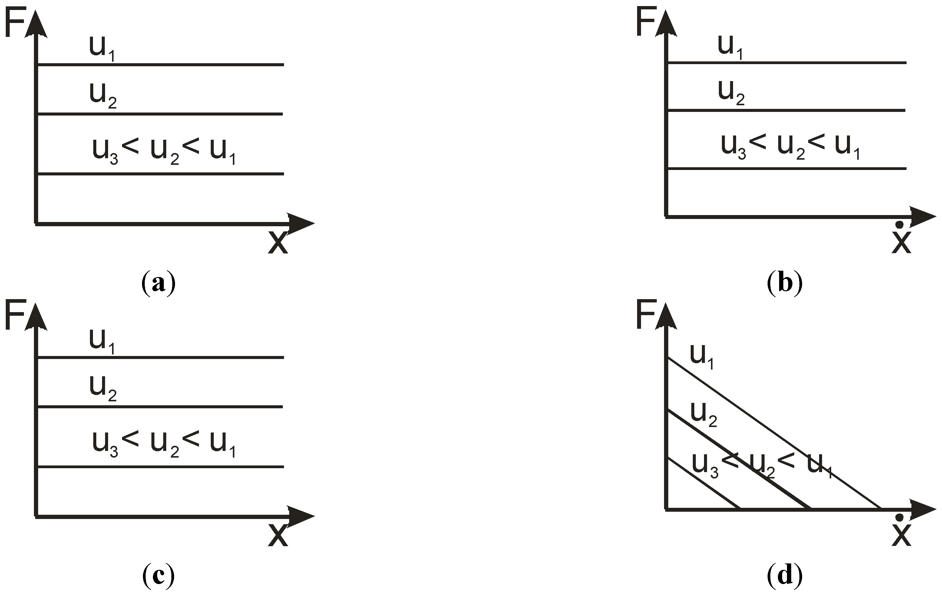
In their paper about actuator properties and movement control, Hannaford and Winters [9] refer to Paynter’s terminology [10] for proposing a definition applicable to any actuator. The authors define actuation as ‘a process of conversion of energy to mechanical form’ and ‘a device that accomplishes this conversion is an actuator’ (page 101). Such an actuator can then be characterized, in Paynter’s theoretical frame, by a double effort-flow and effort-displacement relation where effort is interpreted as a force or torque and flow is interpreted as a velocity. On the other hand, Hannaford and Winter refer to Holmes’ theory [11] to propose a modified version of Holmes’ classification of actuators according to the following scheme: self-induction machines, slip-driven machines, linear-effort controlled machines, linear-flow controlled machines, and concave effort-flow machines. According to the authors, only the last class corresponds to the definition of “muscle-like machines”, in accordance with the so-called force-velocity Hill curve. By considering both force/torque-velocity and force/torque-displacement relationships, the authors characterize the following actuators: internal combustion engine, AC induction motor, DC motor, micro-stepping motor, hydraulic and pneumatic cylinder, McKibben muscle, and human skeletal muscle, but they do not propose any general definition of the artificial muscle. Our approach keeps the double force/torque-velocity and force/torque-position relations for characterizing an actuator but considers an alternative approach to the definition of the actuator understood as a process of energy conversion. The force, or torque, produced by any actuator is used to move a load which can include the mobile parts of the actuator. As a consequence, any relationship force-position and force-velocity peculiar to the actuator results from a second-order linear or non-linear differential equation. A very simple principle results for classifying the actuators: to choose the position, velocity, or acceleration which makes the actuator stable in open-loop with respect to the force or torque it can produce. We, respectively, call acceleration, velocity, or position the three corresponding actuator types. Let us consider a theoretical fluidic cylinder in which friction forces are neglected. It can be modeled by the well-known form: $F=PS=M\ddot{x}$ where S is the cylinder section, M the mobile mass, P the control pressure, and x the resulting position. In a systemic point of view, the corresponding linear system whose input is P and output x is characterized by double poles at the origin and a single zero pole if x-velocity is the output. In both cases, the system is unstable. Its respective force-position and force-velocity characteristics are given in Figure 1a,b. It is important to note that our stability analysis of actuators does not take into account any gravity effect which is considered as an external component of the actuator system. In the case of fluidic cylinders, and more especially for hydraulic cylinders, although the actuator by itself is unstable, an open-loop control is possible in practice by means of a so-called “on-off control” [12] consisting for the operator to open or close valves according to load changes in the links of the machine.

Figure 1. Typical force/position and force/velocity characteristics of an acceleration-type actuator (a) and (b) and of a velocity-type actuator (c) and (d).

Figure 1. Typical force/position and force/velocity characteristics of an acceleration-type actuator (a) and (b) and of a velocity-type actuator (c) and (d).

A DC-electric motor is typically a velocity-type actuator whose force-velocity characteristic can be approximated as drawn in Figure 1d and force-position characteristic is shown in Figure 1c. AC electric motors are also velocity-type actuators but their force-velocity characteristic (see, for example, in [9]) lack the linear character of Figure 1d. It is also clear that any velocity-type actuator is unstable in position. We propose to define any artificial muscle as a position-type actuator i.e., an actuator which is naturally stable in position.

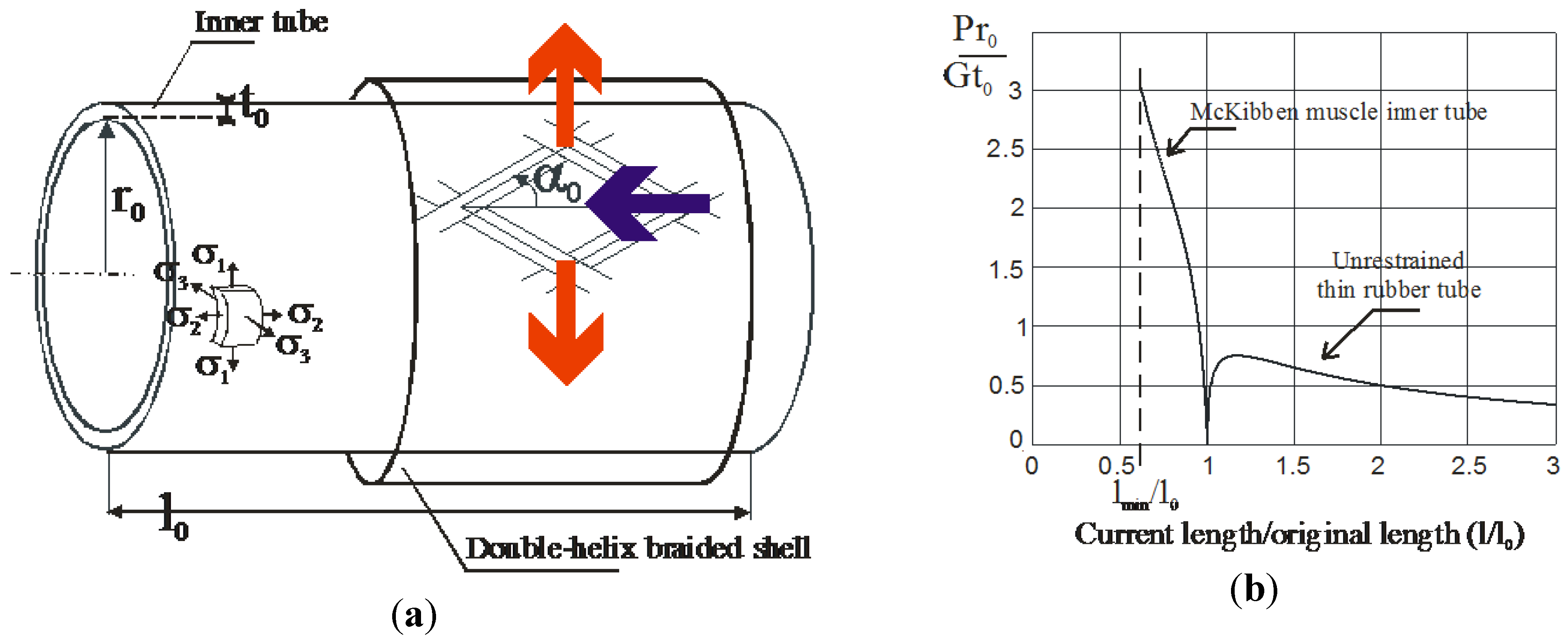
It is important to note that, in this approach, the stability results from an internal process peculiar to the actuator and not from a feedback process based on the use of an adapted sensor—typically, the electromotive force of a DC motor. In the case of artificial muscles, the existence of such an internal stability process has been emphasized as soon the notion of artificial muscle appeared in Kuhn and Katchalsky’s historical research [13]: in his brief report, Katchalsky claims that ‘the equilibrium swelling of the polymeric acid gels is brought about by two opposing tendency: [on the one hand], the solution tendency of the polymeric molecules and the osmotic pressure of the cations of the alkali bound by the gel, [on the other hand], the rubber-type contraction tendency of the stretched polymer molecules’ [14] (page 320). We can also illustrate this fact in the case of the well-known fluidic McKibben artificial muscle whose principle is illustrated in Figure 2a: a rubber inner tube is inflated in some way it can transmit its pressure stress to an external braided sleeve able to transform it into a contraction force. Let us first consider the inflation of the cylindrical inner tube alone. Under the assumption that the pressurized inner tube is a thin cylinder whose initial length, radius and thickness are respectively noted ‘l₀’, ‘r₀’, ‘t₀’, and current length, radius, and thickness are respectively noted, ‘l’, ‘r’, and ‘t’, the expansion of the pressurized cylindrical tube can be derived from classical stress-strain Treloar’s model [15]:

$$\{\begin{array}{c}{\sigma }_1-{\sigma }_2=G({\lambda }_1^2-{\lambda }_2^2)\\ \begin{array}{l}{\sigma }_2-{\sigma }_3=G({\lambda }_2^2-{\lambda }_3^2)\\ {\lambda }_1{\lambda }_2{\lambda }_3=1\end{array}\end{array}\text{ with }\{\begin{array}{c}{\sigma }_1=\mathrm{Pr}/t\\ {\sigma }_2=1/2{\sigma }_1\\ {\sigma }_3=0\end{array}$$

(1)

where λ₁ = (r/r₀), λ₂ = (l/l₀), λ₃ = (t/t₀) and σ₁, σ₂, σ₃ are the corresponding stresses and G is the shear modulus of the rubber. By combining these equations, we derive the following expression linking the inflation pressure P to λ₂:

$$P{r}_0/G{t}_0=2(1/{\lambda }_2)\left[1-(1/(1+\sqrt{1-1/{\lambda }_2^6}))\right]$$

(2)

This relationship, illustrated in Figure 2b, expresses what is well-known by every child trying to inflate a cylindrical rubber balloon: first, the balloon can expand both in radius and length and, secondly, beyond a certain point it becomes easier and easier to inflate it. In other term, a bound-pressure exists that we can be called ‘ballooning pressure’ beyond which the pressure needed to pursue the inflation of the tube is increasingly weak and this ‘ballooning pressure’ equal to about 0.75G(t₀/r₀) is all the more low than the ratio (t₀/r₀) is low. As highlighted by Johnson and Soden [16], this phenomenon clearly corresponds to an instability phenomenon for the rubber tube considered as a system whose input is a control pressure bigger than the ‘ballooning pressure’ and the output is the tube length, as its radius.

If we now consider the same thin cylindrical rubber tube surrounded by a braided sleeve constraining its inflation to follow the two relationships imposed by the geometrical double helix structure of the sleeve [17]: λ₁ = sin(α)/sin(α₀) and λ₂ = cos(α)/cos(α₀) where α₀ and α are, respectively, the initial and current braid angle. We deduce the new relationship:

$$P{r}_0/G{t}_0=2\left[(1/{\lambda }_2)-(\sin {({\alpha }_0)}^2{\lambda }_2)/(1-\cos ({\alpha }_0^2){\lambda }_2^2)\right]$$

(3)

where λ2 varies between a minimum value equal to $\sqrt{1/(3\cos ({\alpha }_0^2)}$ [17] and 1, as illustrated in Figure 2b in the case where α₀ = 20°. It is now clear that the system whose input is control pressure and output the muscle contraction length is stable for any pressure, however, limited by the rubber tensile range.

Figure 2. Interpretation of the braided sleeve movement of the McKibben artificial muscle as the internal process giving to the actuator its artificial muscle nature; (a) combination of the pressurized inner tube and the braided sleeve inside the McKibben structure; and (b) a comparison between the static behavior of an unrestrained thin rubber tube becoming unstable beyond the ballooning pressure and the stable behavior of the McKibben muscle inner tube (see text).

Figure 2. Interpretation of the braided sleeve movement of the McKibben artificial muscle as the internal process giving to the actuator its artificial muscle nature; (a) combination of the pressurized inner tube and the braided sleeve inside the McKibben structure; and (b) a comparison between the static behavior of an unrestrained thin rubber tube becoming unstable beyond the ballooning pressure and the stable behavior of the McKibben muscle inner tube (see text).

Let us make a last comment: in the peculiar case of the McKibben artificial muscle, the braided sleeve is responsible for the open-loop stability in position thanks to the kind of stiffness it gives to the actuator but, in order that this stability is effective, stiffness must be associated to a kind of damping which, for the McKibben muscle, comes from rubber elasticity and in a more important way from kinetic friction inside the braided sleeve.

3. Concept of Linear Artificial Muscle

In order to better understand the link to be made between the proposed concept of artificial muscle and the real skeletal muscle which will be here considered as our biological reference, we propose to introduce an original concept of linear artificial muscle. This linear artificial muscle is considered as a SISO-system whose generated force or torque F has the following general expression:

$$F(u,x)=Ku-b_{0}x-b_1\dot{x}$$

(4)

where K, b₀, b₁ are constants not equal to zero. Let us consider a normalized u-control between 0 and 1 where u = 1 corresponds to a maximum positive force F_max. It can also be assumed that the x-position varies between 0 and a positive x_max-value. If no load is considered, the equilibrium position of the artificial muscle, for a given u-value, is equal to Ku/b₀. Consequently, we deduce: x_max = F_max/b₀. It is then possible to rewrite Equation (4) in the following form:

$$F(u,x)=F_{\max }(u-\frac{x}{x_{\max }})-b_1\dot{x}$$

(5)

It is interesting to note that our definition of the linear artificial muscle can be extended to the definition of a linear velocity-type actuator if it is assumed that b₀ = 0 and to the definition of a linear acceleration-type actuator if b₀ = b₁ = 0, in correspondence with Figure 1. According to the proposed definition, the linear artificial muscle behaves like an “active” spring whose stiffness is constant equal to (F_max/x_max). It is worthy to note that the linear artificial muscle considered in this section, as the biomimetic artificial muscle model considered in next section, are rough approximations of the real behavior of artificial or natural muscles due to the “linear” character—in the meaning of a straight line—of their static characteristics. For example, in the case of the McKibben artificial muscle that has already been mentioned, the isometric force versus muscle x-displacement exhibits a typical convex shape, complicated by a complex hysteresis phenomenon as described by Minh et al. [18], not considered in our study. In a different way, springs made of shape memory alloy, like those fabricated by Kim et al. [19], can exhibit a static characteristic for which a linear approximation of the static force versus deflection at constant temperature appears to be particularly relevant (see in [19], figure in page 81). We did not try, in the framework of this paper, to classify artificial muscles according to the concave or convex shape of their static characteristic, with or without hysteresis phenomenon. We consider, in the spirit of Hogan’s work on the skeletal muscle (see further) that “linear” static characteristics are a simple but powerful way for developing a general model of artificial muscle. More especially in this section, our proposed concept of linear artificial muscle can be considered as an ideal artificial muscle.

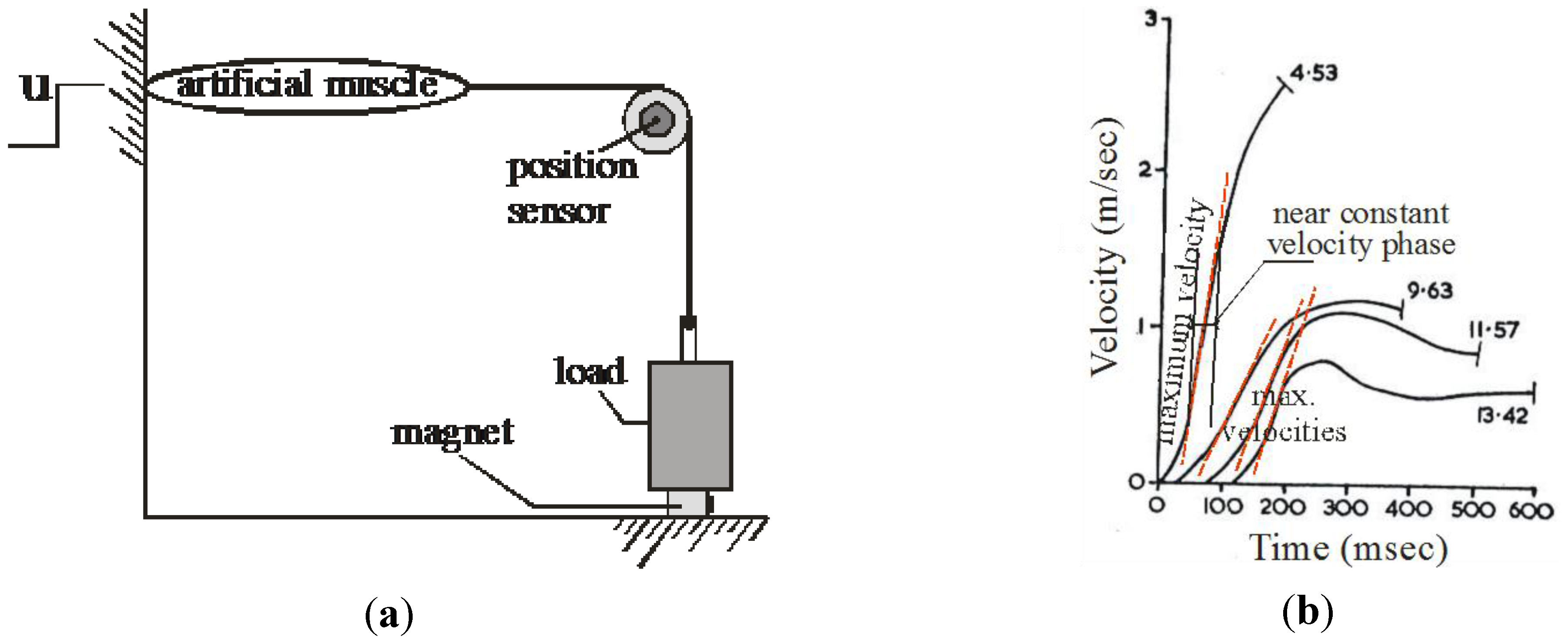
There is, however, a difficulty in this definition of a linear artificial muscle, as also for any definition of an artificial muscle based on the couple force-position and force-velocity: because the x-position is involved in the force expression of the actuator, no evident characteristic force-velocity can be derived by comparison with other actuators. We propose to overcome this difficulty in keeping the well-known Hill curve considered for the skeletal muscle. In his historical 1938 paper [20], Hill indeed proposed a particularly elegant way for characterizing the dynamic behavior of the contractile component of the natural skeletal muscle: to record the velocity during the constant velocity phase just after the beginning of the contraction, produced by a sudden quick-release of a given load. Such a quick-release process can be applied to any artificial muscle and especially to straight artificial muscles, as illustrated in Figure 3a: in a systemic perspective, quick-release is interpreted as a kind of “trial release” from zero position and velocity, applied to the artificial muscle with a constant u-control value and a given load.

Moreover, in the Hill curve, the recorded velocity corresponding to a given load is often interpreted as a maximum velocity during the physiological contraction before it decreases due to the viscosity peculiar to any skeletal muscle, as illustrated in Figure 3b. In accordance with Hill’s spirit, the velocity considered in our pseudo-Hill curve, will be exactly the maximum velocity reached during the “trial release”. It is worthy to note that, although this concept of pseudo-Hill curve can be applied to any kind of artificial muscle for which is specified a privileged “contraction” dimension.

Figure 3. Use of the Hill-curve concept for defining the force-velocity characteristic of an artificial muscle, (a) Hill’s quick-release test considered as a “release trial” of the artificial muscle from zero position and velocity, with a constant u-control and given load, and (b) characterization of the corresponding velocity as the maximum velocity reached during contraction (redrawn from a typical skeletal muscle recording).

Figure 3. Use of the Hill-curve concept for defining the force-velocity characteristic of an artificial muscle, (a) Hill’s quick-release test considered as a “release trial” of the artificial muscle from zero position and velocity, with a constant u-control and given load, and (b) characterization of the corresponding velocity as the maximum velocity reached during contraction (redrawn from a typical skeletal muscle recording).

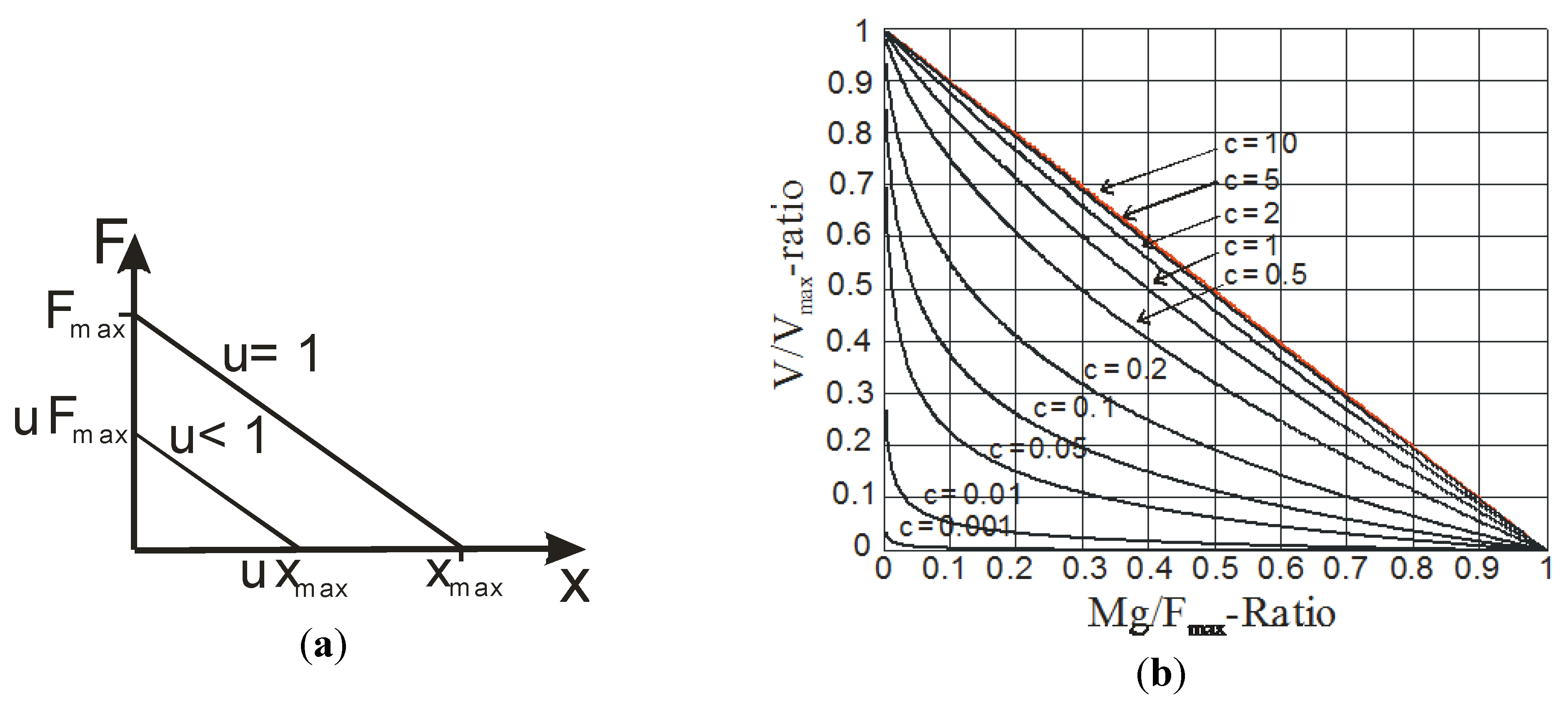
In the case of our linear artificial muscle model, whose static characteristic is shown in Figure 4a, the pseudo-Hill curve is so derived from the look for the maximum velocity of the following dynamic equation:

$$u{F}_{\max }-Mg=M\ddot{x}+b_1\dot{x}+b_{0}x$$

(6)

where M is the considered load. Let us put r_M = Mg/F_max, we get:

$$(u-r_M)=r_M(\ddot{x}/g)+(b_1/F_{\max })\dot{x}+(b_0/F_{\max })x$$

(7)

If r_M = 0, the system behaves like a first order for which maximum velocity noted V_max is given by:

$$V_{\max }=u{F}_{\max }/b_1$$

(8)

If r_M is not equal to zero, we can derive the maximum velocity noted V from the classic solution resulting from the second-order differential equation. It is easy to show that, for a given r_M-ratio, the ratio (V/V_max) only depends on u and the damping Z-factor. We get:

$$\{\begin{array}{c}\begin{array}{l}\text{If Z}<\text{1, }(V/V_{\max }\text{)}=2Z(u-r_M)e^{-\frac{Z}{\sqrt{1-Z^2}}(arctg(\frac{-2Z\sqrt{1-Z^2}}{1-2Z^2})+arctg(\frac{\sqrt{1-Z^2}}{-Z}))}\\ \end{array}\\ \text{If Z}=\text{1, }(V/V_{\max })=2(u-r_M)/e\\ \text{If Z}>\text{1, }(V/V_{\max }\text{)}=2Z(Z+\sqrt{Z^2-1})(u-r_M{\text{)e}}^{-\frac{(Z+\sqrt{Z^2-1})}{2\sqrt{Z^2-1}}\ln (\frac{Z+\sqrt{Z^2-1}}{Z-\sqrt{Z^2-1}})}\end{array}$$

(9)

where the damping Z factor is related to the F_max and x_max parameters of the artificial muscle static characteristic and to the load-ratio r_M by the following relation-ship:

$$Z=c/\sqrt{r_M}\text{ with }c=(\sqrt{g}/2F_{\max })(b_1/\sqrt{b_0})$$

(10)

We give in Figure 4b the set of so-defined force-velocity curves parametrized in c when u is equal to 1. Although our pseudo-Hill curve is not defined as an hyperbolic curve, it is interesting to check that the c-coefficient plays a similar role to the (a/F₀)-coefficient role in the Hill curve: on the one hand, it characterizes the concave curvature of the pseudo-Hill curve and, on the other hand, the lower is c, the more curved is the pseudo-Hill curve, as this is the case for the (a/F₀)-coefficient in the case of the Hill curve. In the bound-case where c tends to infinite, i.e., b₀ tends to 0, the pseudo-Hill curve tends to the straight line: (V/V_max) = (1 − r_M/u). In this case, as previously noted, the actuator lost its artificial muscle nature to be a velocity-type actuator. Moreover, the case c = 1, for which the concave curvature of the pseudo-Hill curve is still little marked, corresponds to the limit for which all “release trials” are performed without overshooting since the limit between underdamping and overdamping is given by Z = 1 and so by: r_M = c². For any c < 1, the time-response will exhibit an overshooting for any load greater than c²F_max/g. Moreover, we would like to show that the linear form of the pseudo-Hill curve can also be considered in the case of a more biomimetic type of artificial muscle.

Figure 4. Linear artificial muscle characteristics; (a) force-position characteristic; and (b) force-velocity characteristic defined as a pseudo-Hill curve (for u = 1)—see text.

Figure 4. Linear artificial muscle characteristics; (a) force-position characteristic; and (b) force-velocity characteristic defined as a pseudo-Hill curve (for u = 1)—see text.

4. Biomimetic Artificial Muscle for Antagonist Actuators

4.1. Biomimetic Artificial Muscle Combining a Non-Linear Static Characteristic with a Linear Viscosity

In his classic paper about impedance control in human movement, Hogan [21] introduced the following simplified static force model of the contractile component of the skeletal muscle we propose to write in a normalized form:

$$F=u{F}_{\max }(1-x/x_{\max })$$

(11)

where F_max and x_max are, respectively, the maximum force and maximum x-contraction corresponding to u = 1, as illustrated in Figure 5a. Although this actuator is clearly non-linear due to the product of u by x, it is always in accordance with our definition of the artificial muscle: whatever the external force generating, for a given u, an equilibrium position x_e, it is obvious that a variation of δx around this equilibrium position produces a return force δF = −(uF_max/x_max)δx and so the actuator stability results. Let us associate to this non-linear static model a linear damping term similar to the one considered in the previous section. During the quick-release process, the value of u-control is constant and it is interesting to remark that for u = 1, which corresponds to the usual physiological conditions of the experimental quick-release under maximal neural activation, the model’s equations become the same for the biomimetic muscle model and the linear one. As a consequence, the curves of Figure 4b can also be considered for the force-velocity characteristic of the biomimetic artificial muscle in the case u = 1. The Hill curve equation can take several forms. We will consider the following one:

$$(P+a)(V+b)=cst$$

(12)

where P is the imposed tension which, according to our notation, is equal to Mg, V is the maximum velocity reached just after the dynamic contraction began, and a, b are constant coefficients characterizing the shape of the Hill curve. This relationship can be written in the following normalized form:

$$(V/V_{\max })=(b/V_{\max })(1-(a/F_{\max })-r_M)/r_M$$

(13)

where r_M = Mg/F_max where V_max is the maximum velocity for no load and F_max is interpreted as the tension producing no displacement i.e., the tension P of Equation (12) which prevents any isotonic contraction of the artificial muscle because this tension is equal to the maximum muscle force F_max. In their paper about biorobotic actuators, Klute, Czerniecki, and Hannaford [22] consider that the (a/F_max)-coefficient characterizing the curvature of the Hill curve belongs to a typical [0.12–0.41] range. In fact, if we take into account other studies, non-considered by the previous authors, this coefficient can reach higher values: a 0.81-value is, for example, considered by Ralston et al. for a human major pectoralis whose data are reproduced in Figure 5b [23]. These last authors also emphasize, at their time, that the (a/F_max)-coefficient is subject to wide variation for a given type of muscle. On Figure 5c, we tried to match the two extreme cases for (a/F_max), 0.12 and 0.81, with a corresponding pseudo-Hill curve as defined in previous section: a c equal to 0.12 has been considered in the case of the Hill curve characterized by (a/F_max) = 0.12 and a c equal to 0.5 has been considered in the case of the Hill curve with (a/F_max) = 0.81. If a certain discrepancy is notable for the lower value in (a/F_max), the concordance between the proposed model and the real data (represented by circles) is rather good for (a/F_max) = 0.81.

Such a relatively good concordance between the Hill curve approaching the real data and the pseudo-Hill curve, derived from a linear viscous friction component, emphasizes, according to us, the great importance of a viscous-like component inside the artificial muscle to get a dynamic behavior close to the one of the skeletal muscle, whatever in fact the chemical or physical origin of such an equivalent viscosity, as this can be checked with authors who tried to apply the force-velocity characterization by the Hill curve to their artificial muscles: Caldwell, for example, designing a so-called pH-muscle by swelling and deswelling a polymer gel inside a hard cylinder [24], or Nakamura et al. designing a pneumatic artificial muscle with straight strings and rings surrounding an inflatable rubber tube [25], or still, the author of this article, in the case of the McKibben pneumatic muscle [26]. Moreover, we considered the real data in load and dimensions (x_max = 9 cm, F_max = 200.1 N) given by Ralston et al. (see table in Figure 5b) for simulating the corresponding time-response of the quick-release—interpreted as a step-response of value u = 1—with c = 0.5. Although real-time responses are not reported in the Ralston et al. article, the authors specify that ‘[the sigmoid character of curves] is always the case expect with very heavy loads, when the curve tends to be flat over a large portion of the excursion’, which is well checked in Figure 5d with a minor overshooting appearing for high loads. Moreover, rising times are in very good accordance with other available experimental results [27]. It is also worthy to note that, in the case of u = 1, the time responses shown in Figure 5d correspond both to the non-linear static characteristic combined with a linear viscous friction and to the full linear artificial muscle model. This suggests that a purely linear artificial muscle, as we defined it, can approach, in a very satisfying way, the dynamic behavior of a real muscle and, therefore, the question arises to know which could be the interest of considering the non-linear static characteristic of Figure 5a instead of the linear one. The answer to this question will be given by the consideration of the actuator made of two antagonist artificial muscles.

Figure 5. Biomimetic artificial muscle and its comparison with the skeletal muscle, (a) force/position characteristic, (b) real data used for the comparison between a human pectoralis major and the proposed biomimetic artificial muscle with a linear viscous damping (rewritten from [23]), (c) comparison between the force/velocity characteristic with u = 1 in two extreme cases of Hill’s curve—the circles correspond to the real data given in (b)—(see text), and (d) time-simulation of the quick-release of the biomimetic artificial muscle in load conditions given in (b).

Figure 5. Biomimetic artificial muscle and its comparison with the skeletal muscle, (a) force/position characteristic, (b) real data used for the comparison between a human pectoralis major and the proposed biomimetic artificial muscle with a linear viscous damping (rewritten from [23]), (c) comparison between the force/velocity characteristic with u = 1 in two extreme cases of Hill’s curve—the circles correspond to the real data given in (b)—(see text), and (d) time-simulation of the quick-release of the biomimetic artificial muscle in load conditions given in (b).

4.2. Constant Moment Arm Antagonist Artificial Muscle Actuator

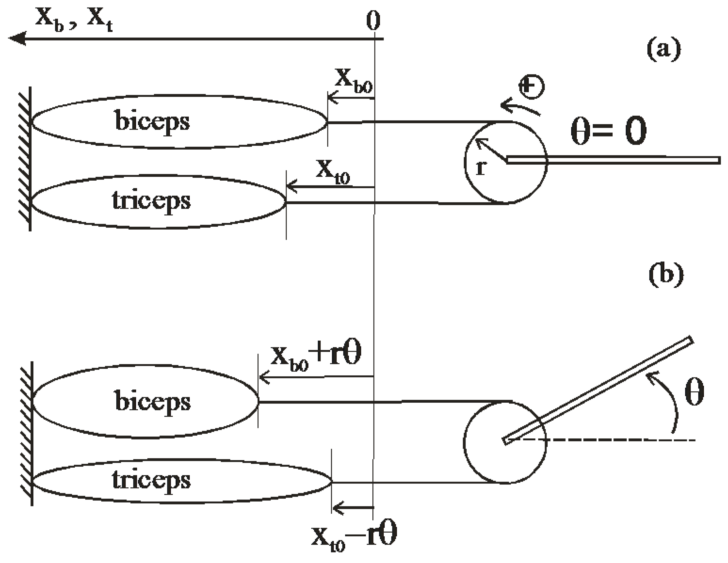
Although some artificial muscles can be considered as bi-directional actuators like bending electro-active polymers, the majority of straight artificial muscles are essentially one-directional actuators. By analogy with muscular physiology, this is an antagonism principle which makes it possible to transform the straight artificial muscle into a bi-directional revolute actuator. A classic way for defining a revolute actuator with two straight artificial muscles consists of linking them by means of an extensible chain and pulley system, as illustrated in Figure 6.

Figure 6. Constant moment arm antagonist actuator, (a) initial state, and (b) current state.

Figure 6. Constant moment arm antagonist actuator, (a) initial state, and (b) current state.

Such an actuator can be said at constant moment arm since the agonist and antagonist muscular actions respectively generate a positive and negative torque with the same and constant moment arm r where r is the pulley radius. We can write the resulting torque T as follows:

$$T=r\left[F_b(u_b,x_b)-F_t(u_t,x_t)\right]$$

(14)

where, by analogy with the animal biceps/triceps system, F_b(u_b,x_b) and F_t(u_t,x_t) are the forces generated by the artificial biceps and the triceps for, respectively, a u_b-control and a x_b-muscle contraction length, and a u_t-control and a x_t-muscle contraction length. If x_b0 are x_t0 are, respectively, the initial x_b and x_t muscle contraction lengths, we have:

$$x_b=x_{b0}+r\theta \text{ and }{x}_t=x_{t0}-r\theta$$

(15)

Assuming that the two muscles are identical, let us first apply Equations (14) and (15) to the linear artificial model considered in Section 3 according to the notation of Equation (5). We easily get:

$$T=(r{F}_{\max })\left[(u_b-u_t)-\frac{(x_{b0}-x_{t0})}{x_{\max }}-\frac{2r\theta }{x_{\max }}\right]-2b_1{r}^2\dot{\theta }$$

(16)

Although its two independent inputs, the actuator behaves like a SISO-system whose equivalent single input u can be written as follows: u = (u_b − u_t) − (x_b0 − x_t0)/x_max where u_b and u_t vary between 0 and 1 and, consequently, u varies between ‘−1 − (x_b0 − x_t0)/x_max’ and ‘+1 − (x_b0 − x_t0)/x_max’. In the case where x_b0 = x_t0, the static characteristic of the actuator takes a particularly simple form, as follows:

$$T_{static}=(r{F}_{\max })\left[u-\frac{2r\theta }{x_{\max }}\right]\text{ with }-1\le u\le +1$$

(17)

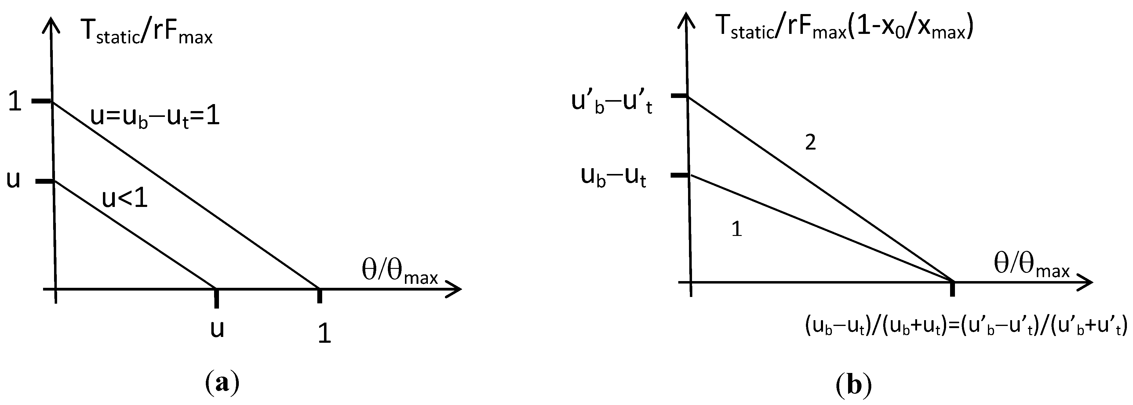
The actuator can then be considered as a bi-directional linear artificial muscle whose constant stiffness is equal to 2r²F_max/x_max and joint angle varies in the range [−θ_max, +θ_max] where θ_max = (x_max/2r). We give in Figure 7a the corresponding torque/angle characteristic in the normalized form T/rF_max versus θ/θ_max, limited to the case of positive actuator angle and torque.

If we now apply Equations (14) and (15) to the biomimetic artificial muscle model of Equation (11) with a linear viscous component whose coefficient is always noted b₁, we get:

$$T=(r{F}_{\max })\left[u_b(1-\frac{x_{b0}}{x_{\max }})-u_t(1-\frac{x_{t0}}{x_{\max }})-(u_b+u_t)\frac{r\theta }{x_{\max }}\right]-2b_1{r}^2\dot{\theta }$$

(18)

The actuator is no more a SISO-system since its two inputs ‘u_b’ and is ‘u_t’ cannot be combined into a single control variable. In the particular symmetrical case in which x_b0 = x_t0 = x₀, the static torque equation is simplified into the following one:

$$T_{static}=(r{F}_{\max })\left[(1-\frac{x_0}{x_{\max }})(u_b-u_t)-(u_b+u_t)\frac{r\theta }{x_{\max }}\right]$$

(19)

In his paper [21], Hogan interprets a similar expression by claiming that (u_b − u_t) is responsible for the actuator torque while (u_b + u_t) is responsible for the joint stiffness. If it is true that, whatever the choice for x_b0 and x_t0, the actuator stiffness is given by ‘(u_b + u_t)(r²F_max/x_max)’ and is so proportional to (u_b + u_t), the other torque component is proportional to (u_b − u_t) only when x_b0 = x_t0 = x₀. In this last symmetrical case, the joint angle varies in the range [−θ_max, +θ_max] where θ_max = (x_max − x₀)/r, and the corresponding static torque can then be rewritten as follows:

$$T_{static}=(r{F}_{\max })(1-\frac{x_0}{x_{\max }})\left[(u_b-u_t)-(u_b+u_t)\frac{\theta }{{\theta }_{\max }}\right]$$

(20)

We give in Figure 7b the corresponding torque-angle characteristic in the case of positive angle and torque: it is clear that the actuator is now able to modify its stiffness—i.e., the slope of its static characteristic—while keeping a given equilibrium position. We can now understand the advantage of the non-linear biomimetic static artificial model by comparison with the linear artificial muscle model: the first one makes possible, when two such muscle models are set into antagonism, to mimic the double nature of the natural joint muscular system as a controller of angle position and angle stiffness.

Figure 7. Torque-angle characteristics for the constant moment arm antagonist actuator, (a) the case of two identical linear artificial muscles, and (b) the case of two identical biomimetic artificial muscles showing the ability of the actuator to modify its angular stiffness (from slope 1 to 2, for example, by increasing the sum of agonist and antagonist control values) while keeping the same equilibrium position (for simplicity reasons we limited our graphs to positive angle and torque).

Figure 7. Torque-angle characteristics for the constant moment arm antagonist actuator, (a) the case of two identical linear artificial muscles, and (b) the case of two identical biomimetic artificial muscles showing the ability of the actuator to modify its angular stiffness (from slope 1 to 2, for example, by increasing the sum of agonist and antagonist control values) while keeping the same equilibrium position (for simplicity reasons we limited our graphs to positive angle and torque).

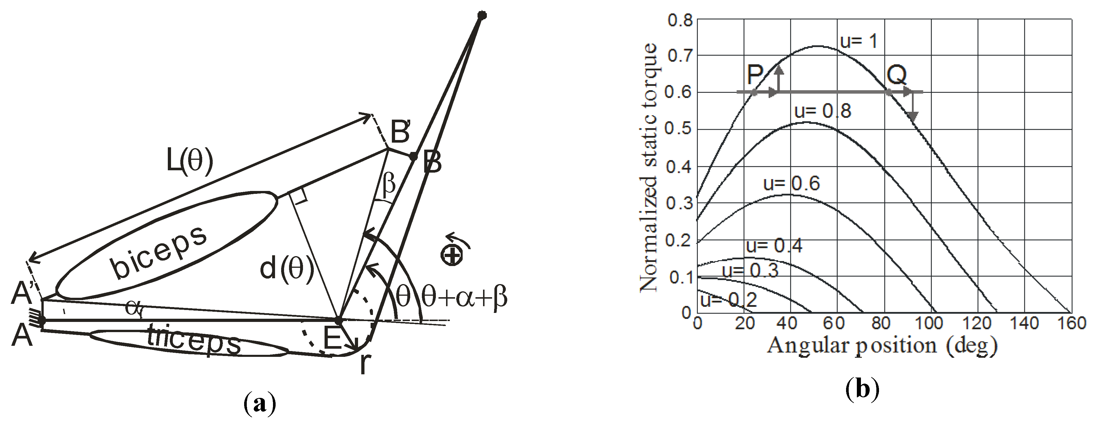
4.3. Elbow-Type Antagonist Artificial Muscle Actuator

The constant moment arm antagonist actuator is, however, an idealized model of a revolute physiological-like joint actuator. We now consider a more realistic model directly inspired from the elbow joint: the antagonist artificial muscle actuator is always made of a biceps and triceps-like straight muscles but the muscles are now directly attached to the links in analogy with the physiological reality. The model is organized as follows. On the one hand, the biceps has its origin in point A’ on the fixed link (arm) and is inserted in B’ on the mobile link (forearm), as illustrated in Figure 8a.

The distance between point A of Figure 8a and elbow joint center E is noted A and the distance between point B and E is noted B. Two offsets are considered, under the form of angles α and β, to express the fact that the distances AA’ and BB’ are not equal to zero in the reality. On the other hand, it is supposed that the ‘tendon’ of the triceps is driven around the elbow joint center with a constant radius r.

Figure 8. Elbow-type artificial muscle actuator, (a) actuator scheme, and (b) corresponding torque-angle characteristic (see text).

Figure 8. Elbow-type artificial muscle actuator, (a) actuator scheme, and (b) corresponding torque-angle characteristic (see text).

Let us note, as previously made, respectively F_b and F_t the forces produced by the biceps and the triceps, θ the elbow joint angle, and T the torque generated by the two muscles. From a simple geometric analysis of Figure 8a, we deduce the following relationships for L(θ) = AB:

$$L(\theta )=\sqrt{A^2+B^2+2AB\cos (\theta +\alpha +\beta )}$$

(21)

As a consequence, the moment arm of the biceps muscle, which corresponds to the distance d from E to the line segment [AB], now depends on the joint angle according to the following relationship:

$$d(\theta )=AB\sin (\theta +\alpha +\beta )/L(\theta )$$

(22)

We deduce the following torque expression:

$$T=T_b-T_t\text{ with }{T}_b=d(\theta )F_b\text{ and }{T}_t=r{F}_t$$

(23)

It is assumed, by analogy with the human elbow joint, that the joint angle θ varies from 0 to a θ_max-value lower than 180°. It is also assumed that, in the zero-joint angle position, the triceps is fully contracted—i.e., its x_b-position is equal to x_max—while the biceps is not contracted—i.e., its x_t-position is equal to 0. In order to make easier the computation of the actuator torque, it is considered that the biceps can contract at least of a x_max-length and so the following expression for the maximum joint value θ_max is deduced: θ_max = (x_max/r). It is worthy to note that no passive tension is taken into account in our model. By applying the non-linear static model of Equation (11) to the artificial biceps and triceps force expressions, we get:

$$\{\begin{array}{c}{F}_b=u_b{F}_{\max }(1-\frac{L(0)-L(\theta )}{x_{\max }})\\ F_t=u_t{F}_{\max }(\frac{\theta }{{\theta }_{\max }})\end{array}$$

(24)

The torque produced by the triceps is given by: $T_t=u_t(r{F}_{\max })(\theta /{\theta }_{\max })$ and, by combining Equations (21) to (24), we get the following expression for the torque produced by the biceps:

$$\begin{array}{l}{T}_b=\frac{u_b{F}_{\max }B\sin (\theta +\alpha +\beta )}{L_n(\theta )}\left[1-\frac{A}{x_{\max }}(L_n(0)-L_n(\theta ))\right]\\ \text{ with }{L}_n(\theta )=\sqrt{1+{(\frac{B}{A})}^2+2(\frac{B}{A})\cos (\theta +\alpha +\beta )}\end{array}$$

(25)

In order to compare the two antagonist actuators, we propose to choose the B-dimension in order that the maximum moment arm of the biceps is equal to r. It is easy to check that d(θ) is maximum for $\theta =\text{atan2}(\sqrt{1-{(B/A)}^2},-(B/A))$ and that this maximum is equal to B. By putting B = r in Equation (25) and by considering the expression of θ_max, we get the new expression for the biceps torque:

$$T_b=(r{F}_{\max })\frac{u_b\sin (\theta +\alpha +\beta )}{L_n(\theta )}\left[1-\frac{L_n(0)-L_n(\theta )}{(B/A){\theta }_{\max }}\right]$$

(26)

Both T_b and T_t-expressions are now proportional to rF_max and we can then define the normalized corresponding total torque T/rF_max = (T_b − T_t)/(rF_max) as we did it for the constant arm antagonist actuator. We give in Figure 8b the corresponding static torque-angle characteristic of the elbow-type actuator for α = β = 10°, θ_max = 180° − α − β, (B/A) = 0.2 and by imposing (u_b + u_t) = 1—the input u_b is denoted u on the graph. By comparison with the torque-angle characteristic shown in Figure 7b, the new static characteristic no longer exhibits a uniformly decreasing slope in the θ-range corresponding to a given constant u-value. Let us consider, for example, the case u = 1 and let us assume that the actuator is submitted to a constant resistive torque: a double equilibrium position can result from such a situation corresponding in Figure 7b to the points P and Q. If the system is set in Q and if it removed from this equilibrium position, for example, by a positive angular variation, its restoring torque is negative, as illustrated in Figure 7b, leading the actuator to asymptotically come back to Q but, if the actuator is set in the equilibrium position P, the restoring torque, corresponding to the same positive angular variation, is now positive with, as a consequence, to move the actuator to the point Q. While Q is an asymptotically stable equilibrium position, P is only an astatic equilibrium position.

5. Conclusions

The systemic approach of the actual notion of artificial muscle we tried to defend in this article is based on a simple and general observation: any actuator privileges a dimension, in position, velocity, or acceleration, with respect to which it is stable. By comparison with classic actuators, artificial muscles define a new type of actuators whose positioning is naturally stable. This open-loop stability in position is the consequence of some internal process whose diversity makes the actual diversity of artificial muscle technology.

The well-known second order linear system can so be interpreted as the dynamic equation of a linear artificial muscle relating its force or torque to its position by means of its gain with respect to a given stimulus, its stiffness and its viscosity. Since the so-called force/velocity characteristic of any artificial muscle cannot be defined in a simple way, as done for a classic actuator, we propose to define it as a pseudo-Hill curve expressing the maximum velocity reached during “contraction” versus the load the artificial muscle has to lift against gravity. In the case of our linear artificial muscle, we show that the pseudo-Hill curve can be parametrized in only one c-parameter depending on static x_max, F_max and viscosity coefficient peculiar to the considered artificial muscle model. We also show that our linear artificial muscle model can relatively well approach the Hill curve of a real skeletal muscle by means of a judicious c-coefficient.

However, a non-linear static force/position characteristic is necessary for making possible an artificial muscle antagonist actuator whose stiffness and angular position can be independently controlled by means of the two independent artificial muscle inputs. Moreover, if this antagonist actuator is designed according to a typical elbow-type joint structure—i.e., without the artificial muscle moment arms both being constant—the corresponding static characteristic lost the uniformly decreasing slope obtained in the case of the constant moment arm antagonist actuator with, as a consequence, the existence of both asymptotic and astatic equilibrium positions.

We hope that, beyond its speculative approach, this analysis could bring help for interpreting and comparing static and dynamic behaviors of artificial muscles.

References

- Madden, J.D.W.; Vandesteeg, N.A.; Anquetil, A.; Madden, P.G.A.; Takshi, A.; Pytel, R.Z.; Lafontaine, S.R.; Wieringa, P.A.; Hunter, I.W. Artificial muscle technology: Physical principles and naval prospects. IEEE J. Ocean. Eng. 2004, 29, 706–728. [Google Scholar] [CrossRef]
- Shahinpoor, M. Ionic polymer-conductor composites as biomimetic sensors, robotic actuators and artificial muscles—A review. Electrochim. Acta 2003, 48, 2343–2353. [Google Scholar] [CrossRef]
- Bar-Cohen, Y. Biomimetics using electroactive polymers (EAP) as artificial muscles—A review. J. Adv. Mater. 2006, 38, 3–9. [Google Scholar]
- O’Halloran, A.; O’Malley, F.; McHugh, P. A review on dielectric elastomer actuators, technology, applications, and challenges. J. Appl. Phys. 2008, 104. [Google Scholar] [CrossRef]
- Tondu, B. Artificial muscles for humanoid robots. In Humanoid Robots: Human-like Machines; Hackel, M., Ed.; Itech: Vienna, Austria, 2007; Chapter 5; pp. 642–677. [Google Scholar]
- Kuribayashi, K. Criteria for the evaluation of new actuators as energy converters. Adv. Robot. 1993, 7, 289–307. [Google Scholar] [CrossRef]
- Huber, J.E.; Fleck, N.A.; Ashby, M.F. The selection of mechanical actuators based on performances indices. Proc. R. Soc. London A 1997, 453, 2185–2205. [Google Scholar] [CrossRef]
- Hunter, I.W.; Lafontaine, S. A comparison of muscle with artificial actuators. In Proceedings of the 5th Technical Digest of the IEEE Solid-State Sensor and Actuator Workshop, Hilton Head Island, SC, USA, 22–25 June 1992; pp. 178–185.
- Hannaford, B.; Winters, J. Actuator properties and movement control: Biological and technological models. In Multiple Muscle Systems: Biomechanics and Movement Organization; Winters, J.M., Woo, S.L.-Y., Eds.; Springer-Verlag: New York, NY, USA, 1990; Chapter 7; pp. 101–196. [Google Scholar]
- Paynter, H.M. Analysis and Design of Engineering Systems; MIT Press: Cambridge, MA, USA, 1961. [Google Scholar]
- Holmes, R. The Characteristics of Mechanical Engineering Systems; Pergamon: Oxford, UK, 1977. [Google Scholar]
- On/Off or Closed-Loop Control? Hydraulics & Pneumatics. Available online: http://hydraulicspneumatics.com/200/TechZone/SystemIntrumen/Article/False/12850/TechZone-SystemInstrumen (accessed on 1 December 2015).
- Kuhn, W.; Hargitay, B.; Katchalsky, A.; Eisenberg, H. Reversible dilatation and contraction by changing the state of ionization of high-polymer acid networks. Nature 1950, 165, 514–516. [Google Scholar] [CrossRef]
- Katchalsky, A. Rapid swelling and deswelling of reversible gels of polymeric acids by ionization. Experientia 1949, 5, 319–320. [Google Scholar] [CrossRef] [PubMed]
- Treloar, L.G.R. The Physics of Rubber Technology; Oxford University Press: Oxford, UK, 1958. [Google Scholar]
- Johnson, W.; Soden, P.D. The discharge characteristics of confined rubber cylinders. Int. J. Mech. Sci. 1966, 8, 213–225. [Google Scholar] [CrossRef]
- Tondu, B. Theory of an artificial pneumatic muscle and application to the modelling of McKibben artificial muscle. CRAS série II 1995, 320, 105–114, (in French with an abridged English version). [Google Scholar]
- Minh, T.V.; Tjahjowidodo, T.; Ramon, H.; Van Brussel, H. A new approach to modeling hysteresis in a pneumatic artificial muscle using the Maxwell-slip model. IEEE/ASME Trans. Mechatron. 2010, 16, 177–186. [Google Scholar] [CrossRef]
- Kim, B.; Lee, S.; Park, J.-H. Design and fabrication of a locomotive mechanism for capsule-type endoscope using shape memory Alloys (SMAs). IEEE/ASME Trans. Mechatron. 2005, 10, 77–86. [Google Scholar] [CrossRef]
- Hill, A.V. The heat of shortening and the dynamic constants of muscle. Proc. R. Soc. Part B 1938, 126, 136–195l. [Google Scholar] [CrossRef]
- Hogan, N. Adaptive control of mechanical impedance by coactivation of antagonist muscles. IEEE Trans. Autom. Control 1984, AC-29, 681–690. [Google Scholar] [CrossRef]
- Klute, G.K.; Czerniecki, J.M.; Hannaford, B. Artificial muscles: Actuators for biorobotic systems. Int. J. Robot. Res. 2002, 21, 295–309. [Google Scholar] [CrossRef]
- Ralston, H.J.; Polissar, M.J.; Inman, V.T.; Close, J.R.; Feinstein, B. Dynamic features of human isolated voluntary muscle in isometric and free contractions. J. Appl. Physiol. 1949, 1, 526–533. [Google Scholar] [PubMed]
- Caldwell, D.G. Natural and artificial muscle elements as robot actuators. Mechatronics 1993, 3, 269–283. [Google Scholar] [CrossRef]
- Nakamura, T.; Saga, N.; Yaegashi, K. Develoment of a pneumatic artificial muscle based on biomechanical characteristics. In Proceedings of the 2003 IEEE International Conference on Industrial Technology, Maribor, Slovenia, 10–12 December 2003; pp. 729–734.
- Tondu, B. McKibben artificial muscle can be adapted to be in accordance with the Hill skeletal muscle model. In Proceedings of the 1st IEEE/RAS-EMBS International Conference on Biomedical Robotics and Biomechatronics (BioRob), Pisa, Italy, 20–22 February 2006; pp. 714–720.
- Fenn, W.O.; Marsh, B.S. Muscular force at different speeds of shortening. J. Physiol. 1935, 85, 277–297. [Google Scholar] [CrossRef] [PubMed]
© 2015 by the authors; licensee MDPI, Basel, Switzerland. This article is an open access article distributed under the terms and conditions of the Creative Commons Attribution license (http://creativecommons.org/licenses/by/4.0/).
Share and Cite
MDPI and ACS Style
Tondu, B. What Is an Artificial Muscle? A Systemic Approach. Actuators 2015, 4, 336-352. https://doi.org/10.3390/act4040336
AMA Style
Tondu B. What Is an Artificial Muscle? A Systemic Approach. Actuators. 2015; 4(4):336-352. https://doi.org/10.3390/act4040336
Chicago/Turabian StyleTondu, Bertrand. 2015. "What Is an Artificial Muscle? A Systemic Approach." Actuators 4, no. 4: 336-352. https://doi.org/10.3390/act4040336