Spatially Nonuniform Heating and the Nonlinear Transient Response of Elastomeric Photomechanical Actuators

Abstract

Recently various nanomaterials, such as carbon nanotubes and graphene, have been added to rubbery elastomers, such as poly dimethyl siloxane (PDMS), to enable generation of stress and displacement in response to remote illumination. While the response is primarily due to heat-induced generation of stress; i.e., the thermoelastic effect in rubbers, illuminated samples have shown unexpected deviations between the transient waveforms of sample temperature and induced stress. In this report we have created a new and simple lumped element model to explain the stress behavior of these photomechanical nanocomposites. The model consists of two parameters that describe the spatially averaged steady state temperature rise due to optical absorption of the structure (typically a long strip of pre-strained elastomer) and the spatially averaged convective cooling rate of the strip, together with a time-varying function that effectively represents the temperature distribution and thermal convection along the length of the strip. The model is used to compare two actuators that each have a thin embedded layer of carbon nanotubes, in which the one film consists of randomly aligned nanotubes and the other has a much more ordered alignment. The model not only fits both transient responses, but the differences between the parameters suggests that the ordered film conducts heat across the strip more rapidly than the disordered film, leading to it more rapidly reaching the steady state level of maximum stress. This model should be helpful in future experimental studies that work to observe, delineate and identify possible nanoscale and molecular contributions to photomechanical stress.

1. Introduction

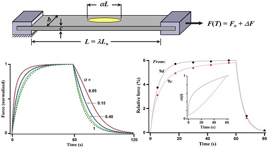
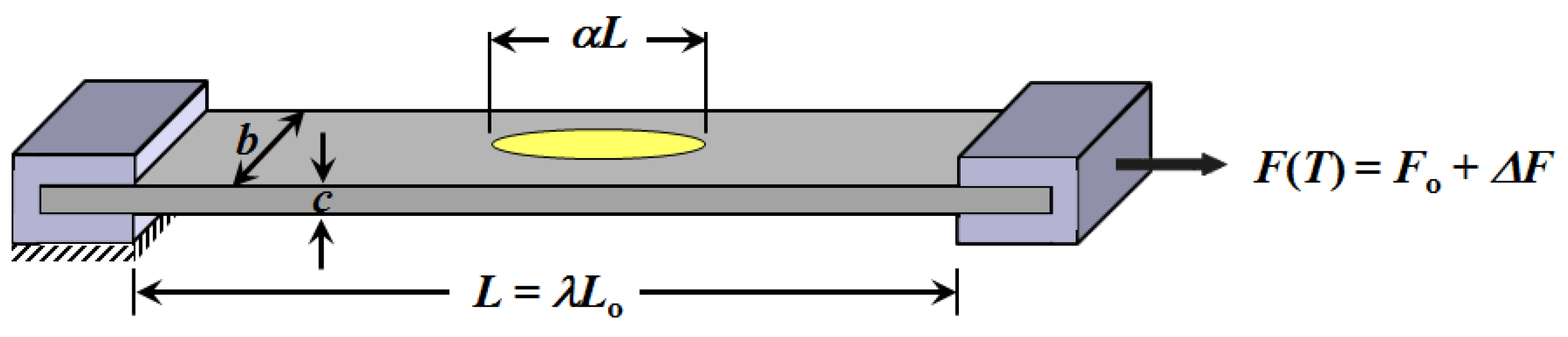
Elastomers, when mixed with even very low concentrations of nanomaterials such as carbon nanotubes, graphene and exfoliated molybdenum disulfide, become photomechanically responsive [1,2,3,4,5]. Remote optical illumination of these composites with LEDs or lasers (as in Figure 1) produces photomechanical stress transients with response times observed to last from a few to tens of seconds. These nanocomposites have been used as remote optically stimulated actuators in a number of micromechanical devices including micro-grippers [6,7], variable tilt micro-mirrors [8], micro-pumps [9] nanopositioning translation stages [10] and even motors based on the chirality distributions of nanotubes [11]. The magnitude of stress produced has been observed to differ with the nanomaterials used, their concentrations, their atomic arrangements and their configurations. For example, a layered film of nanotubes laminated in an elastomer sandwich produces greater stress than if the same amount of nanotubes is uniformly dispersed [12]. Additionally, if the nanotubes are well-aligned in the film, a photomechanical actuator attains its maximum, steady state stress level faster than if the nanotubes are randomly aligned in the film [12].

In these nanocomposite based photomechanical actuators, the stresses produced are principally due to the thermoelastic effect, which is that the force produced by a length of stretched rubber is proportional to temperature [13]. One can get expansion at small strains (3%–9%), zero stress (9%–15%) and contraction (15%–60%) through near infra-red (NIR) illumination [1]. The change in stress is usually 10–50 kPa depending on the pre-strains and is the useful work done by the actuator [1,5]. What makes this an interesting area of study is that the stress transients are different when heated by a filament as supposed to irradiation with light [14]. The NIR illumination typically results in faster stress response compared to simple heating a rubber using a heating element. It was suggested that enormous and instantaneous local temperature increases around individual nanotubes, and finite stress relaxation times that are inherent in rubbers and elastomeric materials might account for this unexpected behavior. The speed of the stimulated response was faster than Debye relaxation, instead following a compressed-exponential law [15]. However, the relaxation after switching off the light source follows the simple-exponential relaxation, as does the stimulated response at very low nanotube concentration [15]. In the reported actuators in the literature, the illumination of light is often a consideration. For example, the stress reported in the literature, some of them illuminate the sample more uniformly along the sample [1], while others have only illuminated the sample in a small area around the center to create a macroscopic photomechanical response [5]. This may suggest uniform and non-uniform heating of the sample, creating macroscopic photomechanical response. The thermal mass of the clamps, interface thermal resistance and convective cooling rates are not described suggesting that the sample may indeed be non-uniformly heated in the reported actuators in the literature.

The question we seek to answer in this report is: Can the observed stress transients be modeled as an entirely thermal effect? More specifically, under the assumption that the relatively slow (on the order of seconds) stress response equilibrates with the instantaneous temperature of the sample, is the stress transient a purely thermal; i.e., equilibrium thermoelastic effect? The model presented herein shows that such a possibility exists if the sample is non-uniformly heated.

This model is specifically applied to the experimental geometry and illumination conditions in Figure 1 (in which the remote optical illumination by LEDs or laser typically have elliptical footprints) [12]. The model proves sufficient to match the observed “compressed exponential” stress transient [15] that occurs simultaneously with a purely exponential thermal transient. The deviation between the stress and thermal transients is a direct consequence of the force equilibration between the hotter (higher stress) and cooler (lower stress) regions of the actuator strip. The model provides a baseline that could help to more clearly study and identify additional influences on the transient response, such as the influence of nonuniform localized microscopic heating effects.

We present a simple model as is realistic and that appears to give an “effective” response that could be easily adjusted to fit measured or rigorously simulated results. This model represents the force generation by two actuator strips in tandem. One strip is uniformly heated by the absorbed optical power, and the other remains at room temperature. To account for thermal conduction along the length of the actuator, the length of the heated strip increases and the unheated strip decreases in time. The transient heating together with the time-varying change in length of the strip that is heated determine the stress transient. The model is developed in three stages, starting by describing the stress produced generated for a fixed quantity of heat as a function of the fraction of the length of the strip that is heated. This model also describes the actuation (the displaced distance) of the hot-cold boundary and the efficiency of photomechanical energy conversion. Then the stress transient is modeled for continuous heating of a fraction of the strip, but with no thermal conduction. With the inclusion of thermal conduction, the model is shown to closely fit, as well as clearly capture the differences between, the photomechanical actuation of strips made with randomly aligned and well aligned nanotube films.

2. Lumped Model 1: Uniform Heating of a Fraction of Length of the Strip

The model treats an elastomeric strip of length L_o as composed of a left part of length L_Lo = αL_o and a right part of length L_Ro = (1 − α)L_o. Prior to heating, the elastomer is elongated to and rigidly clamped at length L = λL_o = (1 + ε)L_o where ε is the strain. We have chosen to represent the force needed to produce this elongation by the introductory model of rubber elasticity [13] as:

$$F=\frac{nkT}{L_{\mathrm{o}}}(\mathsf{\lambda }-\frac{1}{{\mathsf{\lambda }}^2})=G\mathsf{\lambda }{A}_{\mathrm{o}}(1-\frac{1}{{\mathsf{\lambda }}^3})$$

(1)

where n is the number of crosslinks in the elastomer, k is Boltzmann’s constant and T is temperature. In the second equality G is recognized as the shear modulus of the rubber and A_o is the cross sectional area of the strip prior to stretching, which also gives the (engineering) stress of σ = F/A_o. It should be noted that for uniaxial loading the nominal force-stretch relationship for neo-Hookean/Gaussian solid is given by the first part of Equation (1). Equation (1) can be approximated as F = 2C₁₀ $(\mathsf{\lambda }-\frac{1}{{\mathsf{\lambda }}^2})$ where C₁₀ = nkT/2 [16]. For small strains, the second part of equation 1 can be approximated as the Rivlin equation [17]. At large deformations, the observed stress–stretch relationships significantly deviates from the Gaussian model, which is known to be more accurately captured by the 3-chain model (except biaxial data) [16], 8-chain Arruda-Boyce model [18] and Mooney-Rivlin equation [17,19]. However, even these models, which can be fit to the properties of elastomers filled with nanomaterials or formed into layered composites with nanomaterials, can have deviations. Specifically, if carbon nanotubes are mixed into rubbery elastomers, the interfacial shear stress and the shear modulus will change as a function of distribution. The large surface area of nanotubes creates a large interfacial region that can have properties different from the bulk matrix [20]. Chemical bonding between the fiber and the matrix can lead to interfacial shear stress as large as 500 MPa [21]. Similarly micro-mechanical interlocking, van der Waals bonding, bundles versus dispersed nanotubes, the effect of surfactants for nanotube filler dispersion can all have an overall impact on the interfacial shear stress, mobility of polymer chains and can have a pronounced effect on the force-stretch equation and photomechanical actuation. Additionally, the basic model of force-elongation in the neo-Hookean/Gaussian model does not capture the non-entropic compressive force that was observed in [12] for small values of elongation and for strain hardening for large elongations. However, in this report, where fits to experiments were performed for moderate values of elongation, Equation (1) is sufficiently accurate for purposes of illustrating the model.

With the right part of the strip maintained at room temperature T_o, the left part is heated to T = T_o + ΔT. The abrupt change in temperature is permitted out of simplicity rather than physical correctness. Therefore, we can consider this to represent a section of actuator that is heated on average by ΔT. If the strip is uniformly heated by ΔT then, from Equation (1), the relative increase in the force is ΔF/F_o = ΔT/T_o where F_o ≡ F(T_o). If only a fraction α of the strip is heated, an identical amount of force is generated. However, the force on the left F_L must decrease and the force on the right that is initially F_R = F_o must increase until the forces are in equilibrium. The interface displaces to the left by an amount δx_eq or equivalently, in terms of Equation (1), the elongation on the left becomes λ_L = λ − δx_eq/L_Lo and λ_R = λ + δx_eq/L_Ro. Equating Equation (1) written for F_R to Equation (1) written for F_L permits the solution for δx_eq. Because δx_eq/L_Lo << 1, the solution can be approximated from a series expansion of force in powers of δx_eq. 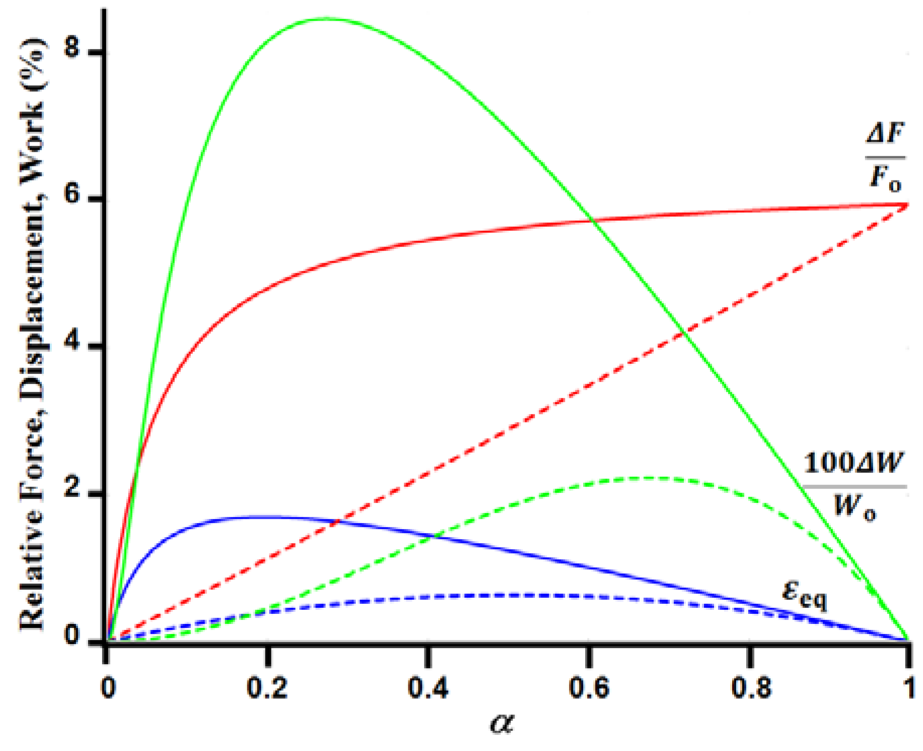With δx_eq determined this way the relative increase in force throughout the strip is:

$$\frac{\Delta F}{F_{\mathrm{o}}}=\frac{\mathsf{\alpha }\Delta T}{T_{\mathrm{o}}+(1-\mathsf{\alpha })\Delta T}=\frac{\mathsf{\alpha } {\mathsf{\eta }}_{\mathrm{c}}}{1-\mathsf{\alpha } {\mathsf{\eta }}_{\mathrm{c}}}$$

(2)

where η_c is recognized as the Carnot efficiency. The relative displacement (of the boundary between hot and cold regions) with respect to the unstretched length of the strip is:

$${\mathsf{\epsilon }}_{\text{eq}}=\frac{\mathsf{\delta }{x}_{\text{eq}}}{L_{\mathrm{o}}}=(1-\mathsf{\alpha })\frac{{\mathsf{\lambda }}^3-1}{{\mathsf{\lambda }}^3+2}\frac{\Delta F}{F_{\mathrm{o}}}$$

(3)

The product of Equations (2) and (3)

$$\frac{\Delta W}{W_{\mathrm{o}}}=\frac{\Delta F \mathsf{\delta }{x}_{\text{eq}}}{F_{\mathrm{o}} L_{\mathrm{o}}}$$

(4)

gives the useful work ΔW performed due to heating with respect to the potential energy W_o in the strip prior to heating. (Note that there is also transfer of potential energy between the left and right side of actuator. That is, the gain in energy on one side is made up by an equal loss on the other side, resulting in no additional work. 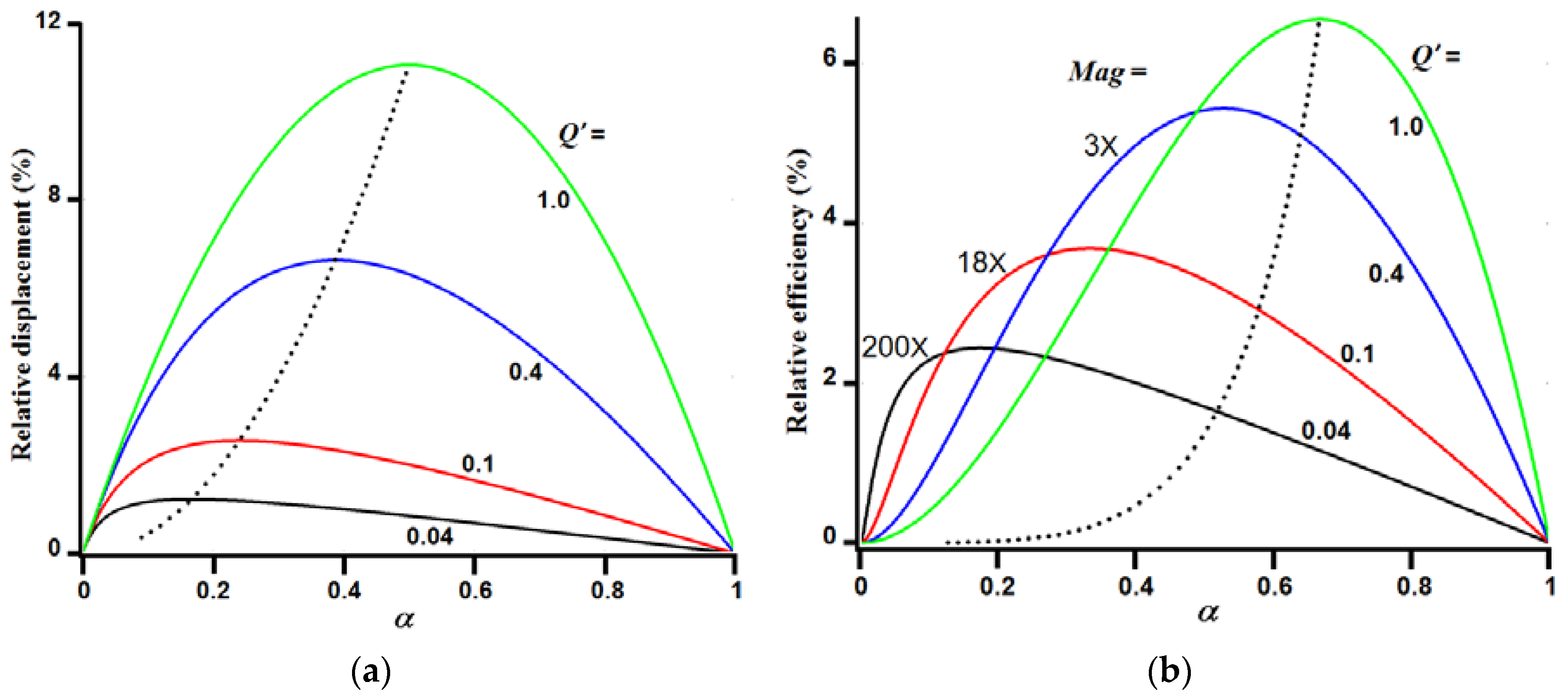This can be seen by considering the total energy of (F_o + ΔF)(L_o + δx_eq)) Equations (1)–(3) are plotted (dashed lines) as a function of α in Figure 2 for an elongation of λ = 1.5 and ΔT/T_o = 17.85/300 (i.e., ~18 °K above room temperature). (Note that the numerical values used in Figure 2, Figure 3, Figure 4, Figure 5 and Figure 6 are based on the actual values used in [12]. For additional details see

Table A1. The table below summarizes the material constants and other parameters used in the plots of Figure 2, Figure 3, Figure 4, Figure 5 and Figure 6. The values were chosen that provide a reasonably close correspondence with the experiments reported in [12].

Variable	Value	Units	Definition	Variable Used in Figure Number	Notes *
λ	1.5		elongation of the strip	2–6
Lo	20	mm	length of strip (unstretched)
bo	3	mm	width of strip (unstretched)
co	0.15	mm	thickness of strip (unstretched)
V = Vo	9	mm3	Volume of strip (stretched or unstretched)	2–6
To	300	K	Temperature	2–6	Standard assumed value for room temperature. Not given in [12]
cpρ	0.00141	J/mm3/K	Heat capacity per unit of volume	2–6	Typical value for Sylgaard PDMS from open literature on density and heat capacity
α	0–1		Fraction of length of the strip that is heated	2–4
	0.05, 0.15, 0.4, 1			5
α(t)	Increasing function of t		Fraction of the length of the strip that is heated	6 in insets	Based on fit to measured data
Pin	45.3	mW	Applied heating rate	5 and 6	From peak stress in Figure 9d, divided by maximum efficiency in Figure 11a (21.9 kPa/0.483 MPa/W)
Q	0.227	J	Applied heat	2	Q(∞) = Pin/β from Equation (15) with β ≈ 5 s from Figure 6 fits
	0.154–3.85			3
	0–5.77			4
Q’	0.0595		Average temperature rise of entire strip relative to To	2	See Equation (5)
	0.04–1.0			3
	0–1.5			4
χ ≡ Q’(∞) ≈ΔF(∞)/Fo	1/6		Average temperature rise of entire strip relative to To at t = ∞ and approximate relative force at t = ∞ when χ << 1	5	Arbitrary value
					Value fit from data for τ in Equation (17):
	0.057			6a	Figure 9c
	0.060			6a	Figure 9d
	0.058			6b	Figure 9c
	0.056			6b	Figure 9d
ΔF(∞)	4.48 (9c)	mN	Maximum (steady state) photomechanical force for continuous heating	6a	Based on Figure 9c,d stress data at 55 s:
	9.80 (9d)			6a
	4.75 (9c)			6b	ΔF(55)
	10.39 (9d)			6b	1.06 × ΔF(55)
τ ≡ 1/β	10	s	Time constant due to convective cooling of the strip	5	Arbitrary value
		s			Value fit for τ from data in:
	4.8			6a	Figure 9c
	5.05			6a	Figure 9d
	4.9			6b	Figure 9c
	4.7			6b	Figure 9d

* Unless otherwise stated the data in this column was taken from [12].

in Appendix).

In addition to plotting the photomechanical response for a fixed temperature increase of the heated portion of the strip, Figure 2 also plots the photomechanical response for a fixed amount of applied heat energy Q. These curves permit one to address the question of how to optimize performance as a function of the fraction of the strip α that is heated by a constant value of Q. Temperature rise is inversely proportional to the length L_L of the heated strip (or, equivalently, volume V_L = αV, where V is the volume of the entire strip), which can be written as:

$$\frac{\Delta T}{T_{\mathrm{o}}}=\frac{Q}{\mathsf{\alpha }{c}_p\mathsf{\rho }V{T}_{\mathrm{o}}}\equiv \frac{Q^{\prime }}{\mathsf{\alpha }}$$

(5)

where c_p is the heat capacity and ρ is the mass density of the material, and V is the volume of the entire strip. Substituting Equation (5) into Equation (2) gives the desired form for the relative force of:

$$\frac{\Delta F}{F_{\mathrm{o}}}=\frac{\mathsf{\alpha }{Q}^{\prime }}{\mathsf{\alpha }+(1-\mathsf{\alpha })Q^{\prime }}$$

(6)

The relative displacement Equation (3) and relative efficiency Equation (4) are unchanged if expressed in terms of ΔF/F_o in Equation (6). These three functions are also plotted in Figure 2 (as solid lines) for Q′ = 17.85/300 (i.e., at α = 1 the solid curves are identical to the dashed curves).

The plots for constant heat show that the maximum force is produced if the entire strip is uniformly heated. However, a sizeable fraction of the force can be produced if only a small fraction of the strip is heated. For example, 80% of the maximum force is realized if only 20% of the strip is heated, which corresponds to the maximum displacement. The maximum work (of ~0.085% of W_o) occurs if 27% of the strip is heated and then around 86% of the maximum force is realized.

If greater amounts of heat are applied, then the peaks of the displacement and efficiency curves shift rightward, as shown in Figure 3. The dashed curves show the shifts in the peaks for the continuous range of values of heat. Basically, as the heat imbalance increases between the two sides of the strip, the peaks move in a direction that tends to reduce the temperature difference. The maximum relative efficiency shown in Figure 3b is 6.5% for Q′ = 1. That is, the strip is, on average, heated to twice the ambient temperature—which is often impractical due to stability and lifetime of many polymeric elastomers at such high temperatures.

Note that relative efficiency used in Equation (4) is only comparing work performed to potential energy stored for the initial room temperature stretching of the rubber. True efficiency compares the work performed to the energy applied (in this case Q, see Equation (5)). Therefore, the true energy efficiency is:

$$\frac{\Delta W}{Q}=\frac{\Delta W}{W_{\mathrm{o}}}\frac{W_{\mathrm{o}}}{Q}$$

(7)

where the relative efficiency ΔW/W_o, is given in Equation (4).

The curve of Equation (6) for relative force in Figure 2 also gives an initial insight into the origin of the force transient. If a fraction α of a strip is initially heated uniformly, then the heat will spread by thermal conduction. In an average sense, this would approximately correspond to the boundary between the hot and cold regions moving, and the value of α increasing. Therefore, over time the strip becomes more uniformly heated and the force increases as shown in the plot of Equation (6).

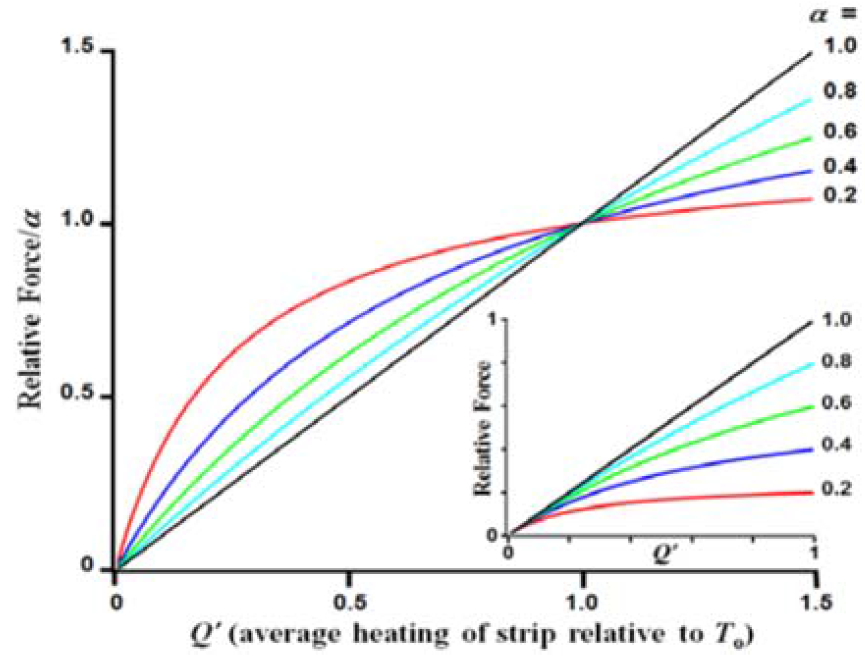
Equation (6) shows that force grows nonlinearly with heating. As shown in Figure 4, heating is only linear with Q’ when the entire length of the strip is heated, and the curves become increasingly nonlinear as smaller lengths of the strip (corresponding to decreasing α) are heated. This nonlinear response appears to contribute in part, in [12], to observed stress transients that do not linearly follow the temperature rise. Additionally, heat spreading (as represented by α increasing with time, as in Figure 2) also can further contribute to a nonlinear relation between stress and temperature.

3. Lumped Model 2: Model 1 with the Addition of Surface Cooling

The analysis to this point has not considered transient effects due to heating and cooling. If a portion of the strip is continuously heated, eventually the heat loss through the sidewalls of the strip will grow until heat increases equal heat losses. In this section we model the heating of the strip with α held constant. This thermal response will be combined with Equation (6) to give the transient force response. Thermal conduction along the length of the strip is not included here, but is added in Section 5.

Equation (6) depends directly on the heat Q added to the sample, since Q’ is directly proportional to Q (Equation (5)). For the heating geometry, which is modeled as being one-dimensional, the heating transient is independent of the length of the strip that is heated. This convenient result follows from the surface area to volume ratio being a constant, as will be shown.

The heating model is for heat applied at a constant rate or power P_in, together with heat loss at the rate P_out(t) which gives overall heating of the sample as:

$$Q(t)=P_{\text{in}}t-{{\displaystyle \int }}_0^t{P}_{\text{out}}(t)dt$$

(8)

For a rectangular strip of unstretched dimensions b_o, c_o and L_o with L_o >> b_o ≥ c_o, most of the heat loss through the heated portion of length L_L will be through the sidewalls transverse to the long direction. The area of the sidewalls is:

$$A_{TL}=2L_L(b+c)=2\mathsf{\alpha }\sqrt{\mathsf{\lambda }}{L}_{L\mathrm{o}}(b_{\mathrm{o}}+c_{\mathrm{o}})\equiv \mathsf{\alpha }\sqrt{\mathsf{\lambda }}{A}_{T\mathrm{o}}$$

(9)

(where we have applied the standard relationships for uniaxial stretching of an incompressible elastomer L = λL_o, b = b_o$/\sqrt{\mathsf{\lambda }}$ and c = c_o$/\sqrt{\mathsf{\lambda }}$, which follows from V = Lbc = L_ob_oc_o = V_o.) The convective heat loss to the surrounding air will be proportional to the heat transport coefficient h, ΔT and A_TL. Using Equations (5) and (9), convective heat loss can be written:

$$\frac{P_{\text{out}}(t)}{T_{\mathrm{o}}}=h\frac{\Delta T}{T_{\mathrm{o}}}{A}_{TL}=h\sqrt{\mathsf{\lambda }}{A}_{T\mathrm{o}}{Q}^{\prime }=\frac{h\sqrt{\mathsf{\lambda }}}{c_p\mathsf{\rho }{T}_{\mathrm{o}}}\frac{A_{T\mathrm{o}}}{V}Q(t)$$

(10)

which shows that the heat loss is independent of α. The heat loss is proportional to the ratio

$$\frac{A_{T\mathrm{o}}}{V}=\frac{2}{c_o}(1+\frac{b_o}{c_o})$$

(11)

which for a fixed volume is minimized when b_o = c_o = $\sqrt{V/L_{\mathrm{o}}}$, or A_To* = 4c_oL_o, where the asterisk indicates the minimum value of surface area. Additionally, for a cylindrical strip of the same volume, the surface area and heating loss is smaller than it is for a square strip by a factor of $\sqrt{\mathsf{\pi }/4}$ = 0.886.

Compared to the experimental devices modeled in this report that has b_o = 3 mm which is much greater than c_o = 0.15 mm, the minimal surface area (for a device of the same volume) would be A_To* ≈ 1.77∙(c_o/b_o)^3/2A_To = 0.02A_To. As can be seen below, not only does reducing the surface area lower transverse heat loss, but the force generated is nearly inversely proportional to the surface area (see Equations (18) and (19)), and the response time is inversely proportional to the surface area (see Equations (13) and (15)). Therefore, in this example where A_To = 50A_To*, while the smaller surface area actuator can produce 50× greater force than the larger surface area actuator for the same rate of heat delivery, the rise time of the smaller surface area actuator would also increase by 50× over the larger area actuator.

Additionally, note in Equation (10) that the elongation λ does increase the surface area which increases the cooling rate. However, also, the cross sectional area of the elastomer strip would decrease by a factor of λ, which reduces heat conduction along the length of the strip. However, in the current study, only one value of λ is considered.

Inserting Equation (10) into Equation (8) gives:

$$Q(t)=P_{\text{in}}t-\mathsf{\beta }{{\displaystyle \int }}_0^{t}Q(t)dt$$

(12)

where

$$\mathsf{\beta }\equiv \frac{h\sqrt{\mathsf{\lambda }}}{c_p\rho }\frac{A_{T\mathrm{o}}}{V}$$

(13)

Equation (12) is equivalent to the linear differential equation:

$$\frac{dQ}{dt}=P_{\text{in}}-\mathsf{\beta }Q$$

(14)

which for initial condition Q(0) = 0 has the solution:

$$Q(t)=\frac{P_{\text{in}}}{\mathsf{\beta }}(1-e^{-\mathsf{\beta }t})$$

(15)

At long times, the steady state condition corresponds Q(∞) = P_in/β where the input power matches the rate of heat loss. If at time t_s the input power is switched off, the solution is:

$$Q(t)=Q(t_{\mathrm{s}})e^{-\mathsf{\beta }(t-t_{\mathrm{s}})}$$

(16)

Combing Equation (15) with Equation (10) (or equivalently, Equation (5)) gives:

$$Q^{\prime }(t)=\frac{1}{c_p\mathsf{\rho }V{T}_{\mathrm{o}}}\frac{P_{\text{in}}}{\mathsf{\beta }}(1-e^{-\mathsf{\beta }t})\equiv \mathsf{\chi }(1-e^{-\mathsf{\beta }t})$$

(17)

From Equations (13) and (17), the constant χ ≡ Q’(∞) can be expressed in terms of basic parameters as:

$$\mathsf{\chi }=\frac{P_{\text{in}}}{h\sqrt{\mathsf{\lambda }}{A}_{T\mathrm{o}}{T}_{\mathrm{o}}}$$

(18)

Equation (17) can be directly substituted into Equation (6) to give the force or stress transient:

$$\frac{\Delta F}{F_{\mathrm{o}}}=\frac{\mathsf{\alpha }\mathsf{\chi }(1-e^{-\mathsf{\beta }t})}{\mathsf{\alpha }+(1-\mathsf{\alpha })\mathsf{\chi }(1-e^{-\mathsf{\beta }t})}$$

(19)

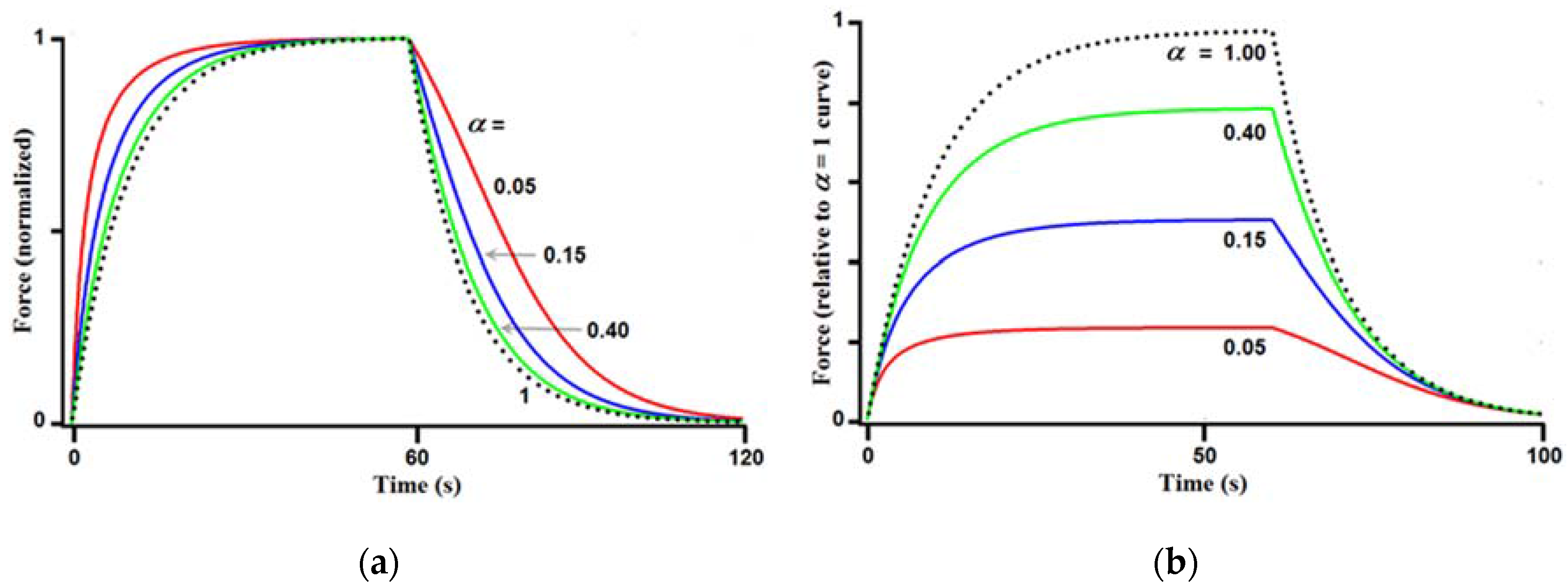
The second term in the denominator causes the stress transient to deviate from the heating transient Q’(t). When α = 1 (a uniformly heated strip) the second term drops out and the shapes of the stress and heating responses are identical. Figure 5 compares Equation (19) to Equation (17) for several values of α (with β = 0.1 s⁻¹ and χ = 1/6, or a 50 K average heating of the strip). Figure 5a shows that the stress waveforms rise faster and fall slower than the heating transient for α < 1. The deviation between the heating waveform and the stress waveform is increasingly pronounced with decreasing values of α. Figure 5b compares the magnitudes of the thermoelastic force for several values of α. The curves show that the maximum force decreases for decreasing α. However, the force decrease is much less than by a factor of α, at least for typical values of χ, which are much less than unity. Specifically, the peak force (from Equation (19)) can be approximately written:

$$\frac{\Delta F}{F_{\mathrm{o}}}\stackrel{t\to \infty }{\to }\frac{\mathsf{\chi }}{1+\mathsf{\chi }(1-\mathsf{\alpha })/\mathsf{\alpha }}\cong \mathsf{\chi }\left[1-\mathsf{\chi }(1-\mathsf{\alpha })/\mathsf{\alpha }\right]$$

(20)

For the case of χ = 1/6 and α = 0.4 the peak force is only decreased 20% from the peak force of the uniformly heated strip.

4. Procedures and Considerations for Applying the Model to Experimental Measurements

Fitting experimental data with Equation (19) can be complicated. First, the value of α is an approximation to a complex and time varying temperature distribution. Experimentally, one could use a thermal imaging camera to measure the thermal profile along the length of the strip and use this to constrain the values of the idealized function α(t). Second, the value of the initially applied force F_o needs to be known. In the experiments in [12], the values of ΔF were reported, but the value of F_o was not. Furthermore, the strip is not a pure elastomer, but rather a laminate of a thin layer of nanotubes (less than one micron thick, to enable high absorption and conversion of optical into thermal energy), sandwiched between two 75 μm thick layers of PDMS rubber. The model does not consider the true elastic properties of this more complicated composite material.

The importance of accurately determining F_o can be appreciated by comparing its value as determined by two different approaches. In [12] the “effective” elastic modulus E of the actuator being modeled here was reported to be about 2.3 MPa. Using the standard relationship for ideal rubber of shear modulus G = E/3 the force per unit area at elongation λ = 1.5 in Equation (1), gives an estimated value of F_o/A_o = 790 MPa. However, if instead we determine F_o/A_o from Equation (20) approximated under the assumption that α is close enough to unity to ignore its contribution we get:

$$\frac{\Delta F(\infty )}{F_{\mathrm{o}}}\cong \mathsf{\chi }$$

(21)

With value of maximum thermal/photomechanical stress measured in [12] as ΔF/A_o = 21.8 kPa, together with χ = 0.06 (estimated is Section 5 from fits to Equation (19)), the stress F_o/A_o = 360 MPa or 46% of the first estimate. In the following section on fitting experimental photomechanical stress data from [12] we will use the second estimate of F_o. To develop a more rigorous correspondence or calibration between experiment and the model, it will be important in future experiments to record F_o and to measure ΔF(∞) for uniform heating (i.e., α = 1). In fact, if the strip is heated uniformly to a known temperature in an oven (rather than by optical illumination), this gives χ = Q’ = ΔT/T_o (see Equations (5) and (17)). Then the value of F_o measured with a force transducer can be compared with F_o determined using Equation (21). Next, the heat source is turned off and the sample is returned to room conditions. The time constant β can then be extracted from the decaying force transient. With β and χ determined by uniform heating, and the parameters c_p, ρ, V, T_o being relatively easy to measure, it becomes possible to use Equation (17) to determine the absorbed optical power, and possibly with better accuracy than by direct optical transmission measurements, as had been used in [12].

The model can be further refined by measuring the force-elongation response of the material, and comparing it with nanotube-free samples. Deviations from the idealized model of rubber elasticity in Equation (1) can be incorporated into revised versions of Equations (2)–(4). Nonetheless, even with these current limitations in the available data sets, we can evaluate the validity and limitations of this approach to modeling, as shown next.

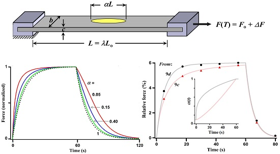
5. Lumped Model 3: Model 2 with the Addition of Thermal Spreading

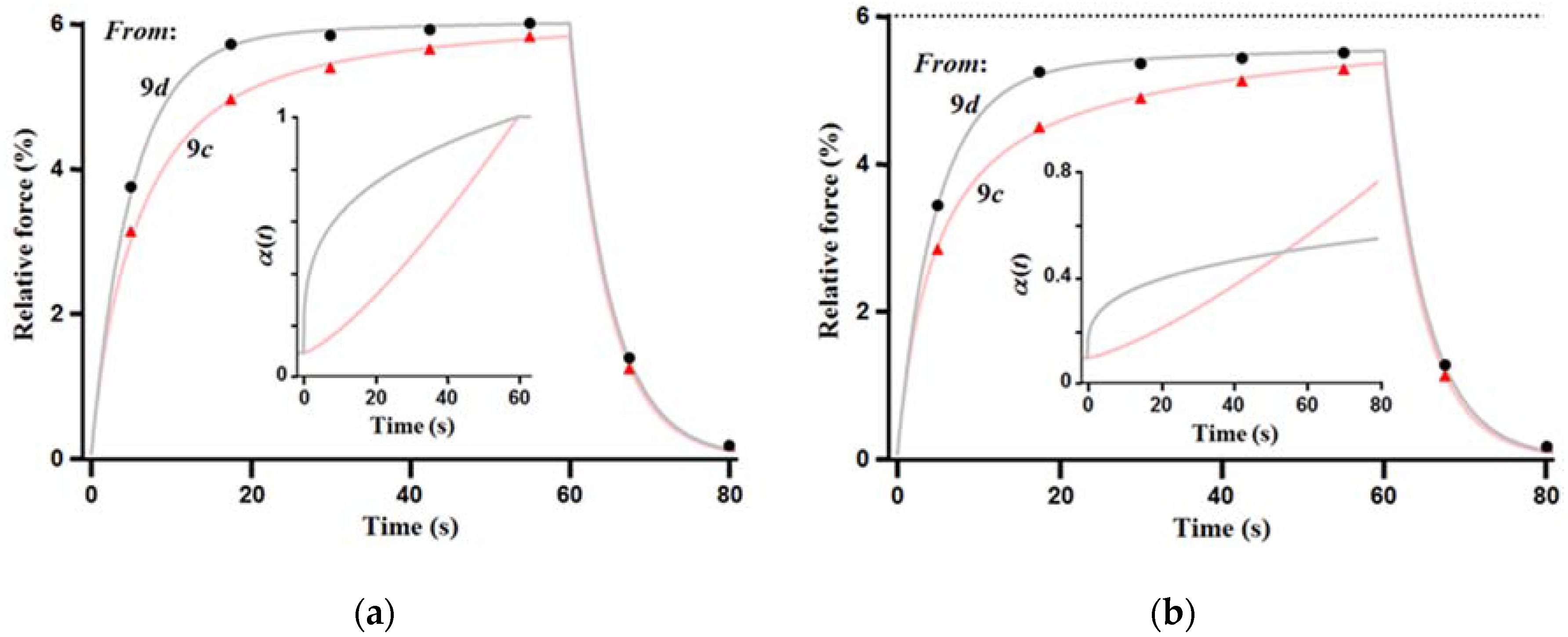
Fittings are made to the responses of the two actuators reported in [12]. Each actuator was made with a thin embedded film of nanotubes and each was elongated by a factor of λ = 1.5. The films differ only on the degree of nanotube alignment or order, with the actuator containing the ordered film producing the greater amount of force when absorbing the same amount of optical power (45.3 mW). Each actuator is irradiated with the identical pattern over about 10% of the stretched length. The data points for the measured transient force responses are plotted in Figure 6. The values are normalized by an estimated value of F_o using Equation (21). Equation (17) shows that the value of χ is a function of the time constant β, with all the remaining terms in Equation (17) being known or measured constants. Therefore, once ΔF(∞) is determined, Equation (19) can be fit to the data sets as a function of β and α(t). Fortunately, χ is on the order of 0.06, so that the largest value of data (at 55 s) is reasonably close to ΔF(∞), even if α(55 s) ≈ 0.5. This can be seen from Equation (20) where for χ = 0.06 then ΔF(∞) is approximately 6% higher than the maximum measured force. In performing the fitting, the value of β (≈1/5 s⁻¹) is fairly easily fit to the falling transient after the heat source is turned off at 60 s. This can be appreciated by considering Equation (16), which replaces the rising exponential function in Equation (19) with a function that is exponentially decaying. The already small denominator term rapidly drops out of the equation. Given the sparse sampling of the data points, any fine deviations from exponential (as in Figure 5a) cannot be resolved. Given how small the deviations are likely to be, it is difficult to see if finer sampling could provide much improvement on the estimated values of the parameters.

Given this relatively small deviation from exponential for the decaying response, we fit the data sets for two different values of ΔF(∞). In Figure 6a the data is fit assuming that ΔF(∞) = ΔF(55 s) and in Figure 6b the data is fit assuming ΔF(∞) = 1.06 × ΔF(55 s). To the eye, the fits to the data in Figure 6a are nearly identical to the fits in Figure 6b. The fits are accomplished using different functions of α(t), which are plotted in the insets. The relative forces in Figure 6b are lower than in Figure 6a by ~6%. (As a guide to the eye, the horizontal dashed line in Figure 6b is included to indicate the maximum relative force achieved in Figure 6a). The magnitudes of α(t) are considerably smaller in Figure 6b than in Figure 6a, being 40%–50% lower at 60 s. The fits also differ somewhat in the value of β used. The value used for Figure 6a were τ ≡ β⁻¹ = 5.05 s for the actuator with the disordered nanotube film, and τ = 4.9 s for the actuator with the ordered film. These time constants change slightly in Figure 6b to τ = 4.7 s for the disordered film and τ = 4.9 s for the ordered film.

The shapes of the α(t) curves differ dramatically between the ordered and disordered samples. Whether this represents the actual heat spreading requires further study, e.g., with a thermal imaging camera, as mentioned above. However, if the curves for our lumped element model do realistically represent heat spreading, then perhaps the difference in the shape of the curves is indicative of increased heat transport along the length of the strip for the ordered film, and increased lateral conduction and convection of heat for the disordered film. If the transient profiles of α(t) are realistic, the difference might arise from enhanced packing of nanotubes and less tortuosity in the ordered film that would increase thermal conduction along the length of the strip, and for the disordered film, increased surface area in contact with the elastomer that would enhance cooling transverse to the length.

6. Discussion

While the model and fitting presented above is designed to represent the work reported in the literature [12], the model might be applicable to modeling results for a uniformly illuminated sample [1] if the thermal boundary conditions at the end clamps were available. The clamps could have a large thermal mass that cools the actuator more at the ends than by convection in the center. The contact area and thermal resistivity between the clamp and sample is also unknown. If the clamps are more effective at cooling than convective cooling from the surface of the actuator, then the thermal profile could be expected to evolve in time as follows: The uniform illumination would produce uniform heating across the strip, leading to maximum stress for a given amount of heat and α would then initially equal 1. With continued illumination the center of the strip would heat faster than the ends of the strip, leading to a thermal distribution that would be peaked at the center of the strip. Therefore, α(t) in the model would actually decrease with time, and less stress would be realized than for a uniformly illuminated sample. (For instance, see inset Figure 4). This seems to suggest that the stress transient at the center of the strip could be slower than the temperature rise. While the experimental reports suggest that thermocouples were attached to the surface of the strip, but the exact location in length was not indicated [1]. If the thermocouples are located close to the clamps, then they could be missing the more rapid heating at the center of the strip. If the thermocouples are closer to the center, higher change in temperature can be observed. When the illumination is removed, the center of the strip (which contributes the most to stress generation) also cools faster, due to a greater temperature difference from ambient, than near the end clamps. Therefore, under the conditions of good heatsinking and thermal monitoring close to the clamps, the measurements would then give the appearance that both growth and relaxation of stress are more rapid than the change in temperature.

This discussion does not invalidate observations of sizeable and rapid stress transients in the experiments reported in the literature, but it does show that until the thermal profile is well described, it will be difficult to quantify more subtle influence of the elastomeric properties and of the added nanomaterials, that could produce macroscopic and nanoscopic changes in thermal, mechanical and potentially, other properties that influence the photomechanical response. For instance, nanotube organization alone is quite varied, from unpercolated and percolated dispersions, to films of various degrees of packing and alignment. These factors alone would have differing effects on elastic modulus, photothermal conversion, thermal conduction and interfacial thermal resistance. The addition of fillers such as carbon nanotubes/graphene in rubbers can add to the elastic instabilities. Materials that undergo large elastic deformations can exhibit novel instabilities [22]. A original article by A.N. Gent has discussed several instabilities for rubber namely aneurysm on inflating a cylindrical rubber tube, non-uniform stretching on inflating a spherical balloon, expansion of small cavities in rubber blocks when they are subjected to a critical amount of triaxial tension or when they are supersaturated with a dissolved gas, wrinkling of the surface of a block at a critical amount of compression, and the sudden formation of “knots” on twisting stretched cylindrical rods [22]. Of this, formation of knots of cylindrical nanotubes, twisting of nanotubes, fragmentation of nanotubes due to non-uniform strain, interfacial bonding/debonding of graphene fillers [23] and effect of dissolved gases inside the nanotubes can lead to elastic instabilities in rubber nanocomposites and can have a profound effect on the thermo-mechanical/photomechanical actuation. These are not currently understood and sophisticated processing techniques combined with modeling approaches can address these challenges in the future. It should be noted that the present model does not account for viscoelastic retardation behavior due to the short time scales involved. While long-term steady-state cycling response showed excellent stability of the photomechanical actuator without any degradation effects both in expansive and contractive actuation modes over 24 h [24], these time scales are not enough to see any creep or hysteresis. The model, thus, is based on quasi-static equilibration of forces. Fitting the lumped element model to experiments that span this full range of nanomaterial addition including geometric effects (1D nanotubes vs. 2D graphene) would be useful for more clearly understanding their influence on the thermal and photomechanical properties, while potentially helping to distinguish other contributing elastic instabilities.

7. Conclusions

The ability to convert light into mechanical motion is bound to impact many energy related applications. This field of photomechanical work generated by polymers and nanomaterials is growing steadily and a suitable and simple analytical model that show case the main effects could be useful in design and development of devices based on these effects. We have developed and presented a simple lumped element model that describes photomechanical stress generation as a thermoelastic effect. This model is motivated by the need to develop a more detailed insight of experiments, and the recognition of the difficulty in fully quantifying all relevant material properties and thermal boundary conditions. The model is described in terms of two parameters χ and β (that depend on a number of material and geometric parameters) and as function α(t) that describes a highly idealized bimodal thermal profile that effectively represents the actual three-dimensional time-varying thermal distribution. These parameters proved to be sufficient to accurately fit the previously reported experiments. However, due to the lack of a missing value of tensioning force, which we used as a free parameter, we were able to fit the data sets equally well for two different sets of the parameters χ, β and α(t). On the other hand, the fact that the experimental device is a layered composite of a thin film of nanotubes between a thick layers of elastomer, the idealized force-elongation response Equation (1) that underlies the model, might require additional modifications beyond simply quantifying the tensioning force. As far as applying the model to future experiments, we also noted that two of the parameters χ, β can be determined by uniformly heating and cooling the sample, say in an oven, which might provide improved control and interpretation of the experiments.

Overall, the lumped model of photomechanical stress transients could be used to provide guidelines for detailed multiphysical simulation, design and experimental characterization of photomechanical actuators. With further refinement of the model and accompanying experimental methods (e.g., heating with intense, short duration light pulses) the model could be help to distinguish the continuum thermoelastic stress response from various molecular and nanoscale effects, e.g., polymeric relaxation times and highly localized heating effects around the embedded nanomaterials.