The Flux-Based Sensorless Field-Oriented Control of Permanent Magnet Synchronous Motors without Integrational Drift

Abstract

The magnitude of the rotor magnetic flux linkage and its spatial orientation within a permanent magnet synchronous motor directly define the angular position of the rotor and are thus used in many sensorless applications as the governing variables. The rotor magnetic flux linkage in the stator reference frame is represented by two orthogonal sinusoids whose amplitudes and phases are determined by the integration of the orthogonal components of the corresponding voltage, which, due to DC offsets and initial conditions at transient states, result in an integrational drift. This paper proposes a solution to the problem of such integrational drift in the form of a compensation based only on orthogonal properties of waveforms in the stator reference frame. That makes it completely independent of electrical parameters of the motor. As a result, the proposed compensation of the integrational drift does not require any optimization by the user and it is functional from a standstill. The effectiveness of the proposed compensation is demonstrated analytically, by a simulation, and an experiment on a real motor by a simple observer for the sensorless field-oriented control based on the voltage model in the stator reference frame.

1. Introduction

Every permanent magnet synchronous motor (PMSM) combined with the field-oriented control (FOC) represents one of the most efficient electro-mechanical systems. Keeping the efficiency on a high level comes at the expense of complex control algorithms that require the angular position of the rotor during the operation. The angular position of the rotor is obtained by a position sensor such as an encoder, a resolver, or a Hall sensor. Such a sensor requires additional space for mounting, proper wiring to avoid interferences with its surroundings, and increases the overall cost of the drive. For that reason, a sensorless implementation of the FOC is a step towards a reduction in costs of drives comprised of PMSMs and an improvement in their reliability. While the position sensor for some reason may stop working, sensorless algorithms work as long as the motor itself together with the power electronics is operational.

Sensorless observers of the angular position and speed of the rotor can be based on the voltage or the current model of the motor. They can be implemented either in the stator reference frame or in the rotor reference frame, although the combination of variables from both reference frames, as presented in [1], is also feasible. This paper focuses on open-loop observers based on the voltage model in the stator reference frame whose governing variable for the calculation of the angular position of the rotor is the rotor magnetic flux linkage. Since the voltage equations of the motor in such observers are being integrated, most of the measurement noise is inherently filtered out. Another advantage comes from the fact that the amplitude of the rotor magnetic flux linkage is constant throughout the speed range up to the nominal speed, which ensures a constant resolution of the reference waveforms from which the angle is being calculated. The main challenge of implementing such an observer represents the compensation of the integrational drift caused by even the smallest DC offsets in the measured input waveforms and initial conditions at transient states that get accumulated by the integration. The requirement of the angular position of the rotor for the transformation of quantities into the rotor reference frame makes the stator reference frame the preferable choice.

A great majority of attempts to overcome the problem of the integrational drift has so far been addressed in the stator reference frame, mostly in applications with squirrel cage induction motors (SCIMs). The simplest approach with integrators is presented in [2] by resetting them after every full electrical period based on the accumulated average value of the integrational drift. While this method works in steady states, its dynamics is severely limited because the accumulated integrational drift in a single period can become too large to be successfully compensated, which consequently results in instability. The integrators are typically replaced by low-pass filters (LPFs), which, from the standpoint of the transfer function, is equivalent to a high-pass filter (HPF) in a cascade with each of the integrators to attenuate DC offsets in the waveforms of the input voltage. From the results of such implementations presented in [3,4,5,6,7,8], it can be seen that the LPFs influence both the magnitude and the phase of the output waveforms of the magnetic flux linkage. While the influence on the magnitude above the cut-off frequency is practically negligible, the phase shift of the LPFs must be compensated because of its direct influence on the estimated angular position of the rotor. Lower values of the cut-off frequency reduce the dynamics as well as the error in the estimated angular position of the rotor, while its higher values have the opposite effects. Based on that notion, cascaded LPFs presented in [9,10] pass the waveforms of the input voltage through the filter whose cut-off frequency satisfies the required dynamics at the operating speed, while the phase shift is being compensated based on the time constant of the selected filter and the instantaneous value of the speed. Computationally more efficient solutions in the form of programmable LPFs with variable cut-off frequencies are presented in [11,12,13,14], where the dynamics can be improved by selecting a suitable ratio of the cut-off frequencies and the instantaneous speed. That also ensures a constant phase shift and, consequently, a constant error in the estimated angular position of the rotor that can be easily compensated through the entire speed range. Nonetheless, all methods mentioned so far require an additional compensation of the phase shift due to the native frequency response of the used LPFs. An attempt to mimic the transfer function of integrators by a combination of two LPFs is presented in [15,16]. Besides a relatively slow rejection of disturbances in transient states that, according to presented results, last between 0.5 s and 1 s from their occurrence, the proposed solutions apparently require a 32-bit implementation primarily due to Cartesian to Polar conversions that contain sums of squared values under square roots. Methods to estimate the magnetic flux linkage using pure integrators are proposed in [17,18,19]. The method in [17] presents a general solution to the problem of the integrational drift, while the methods presented in [18,19] focus on SCIMs at very low speeds. The method in [17] exhibits limited dynamics due to its complexity. That can be seen from the presented step response, where the residual error persist for about 4 s after the occurrence of a transient state. The methods presented in [18,19] are essentially identical and so far the best solution to the problem of the integrational drift regarding the stated duration of transient states that ranges between 250 ms and 280 ms.

This paper addresses the problem of the integrational drift with a simple and straightforward solution based on orthogonal properties of the input and output waveforms of the integrators in the stator reference frame. While all the referred methods require some sort of optimization by the user, the solution presented hereafter requires no optimization due to its complete independence of the electrical parameters of the motor. Consequently, the proposed solution, unlike the referred methods based on LPFs, does not influence the amplitude or the phase of the resulting output waveforms in steady states. The clams stated here are supported analytically and experimentally in the following sections.

2. The Electrical Angular Position and Speed of the Rotor

A PMSM can be characterized by its voltage equation expressed as a function of the torque angle ($\delta$) and time (t). Accordingly, the spatial phasor of the stator phase voltage projected onto the stator reference frame (${\mathit{v}}_{\mathrm{s}\alpha \beta }$) can be expressed in terms of the per-phase stator electrical resistance ($R_{\mathrm{s}}$), the spatial phasor of the stator electrical current projected onto the stator reference frame (${\mathit{i}}_{\mathrm{s}\alpha \beta }$), and the spatial phasor of the stator magnetic flux linkage projected onto the stator reference frame (${\mathit{\lambda }}_{\mathrm{s}\alpha \beta }$) as

$$\begin{array}{ccc}\hfill {\mathit{v}}_{\mathrm{s}\alpha \beta }(\delta ,t)& =& R_{\mathrm{s}}{\mathit{i}}_{\mathrm{s}\alpha \beta }(\delta ,t)+\frac{\partial }{\partial t}{\mathit{\lambda }}_{\mathrm{s}\alpha \beta }(\delta ,t).\hfill \end{array}$$

(1)

By starting from the right-hand side, ${\mathit{i}}_{\mathrm{s}\alpha \beta }$ is defined via the base of natural logarithms (e) and the imaginary unit (j) in terms of the magnitude of the fundamental harmonic of the stator electrical current ($i_{\mathrm{s},1}$), the electrical angular position of the rotor (${\theta }_{\mathrm{e}}$), and $\delta$ as

$$\begin{array}{ccc}\hfill {\mathit{i}}_{\mathrm{s}\alpha \beta }(\delta ,t)& =& i_{\mathrm{s}1}{\mathrm{e}}^{\mathrm{j}\left({\theta }_{\mathrm{e}}\right(t)+\delta )}.\hfill \end{array}$$

(2)

To account for the magnetic saliency of the rotor, ${\mathit{\lambda }}_{\mathrm{s}\alpha \beta }$ is defined in terms of the products of the mean stator inductance ($L_{\mathrm{s},0}$) with ${\mathit{i}}_{\mathrm{s}\alpha \beta }$ and the second harmonic of the stator inductance ($L_{\mathrm{s},2}$) with the complex conjugate of ${\mathit{i}}_{\mathrm{s}\alpha \beta }$ (${\overline{\mathit{i}}}_{\mathrm{s}\alpha \beta }$) with an addition of the rotor magnetic flux linkage constant (${\lambda }_{\mathrm{m}}$) as

$$\begin{array}{ccc}\hfill {\mathit{\lambda }}_{\mathrm{s}\alpha \beta }(\delta ,t)& =& L_{\mathrm{s},0}{\mathit{i}}_{\mathrm{s}\alpha \beta }(\delta ,t)-L_{\mathrm{s},2}{\overline{\mathit{i}}}_{\mathrm{s}\alpha \beta }(\delta ,t){\mathrm{e}}^{\mathrm{j}2{\theta }_{\mathrm{e}}\left(t\right)}+{\lambda }_{\mathrm{m}}{\mathrm{e}}^{\mathrm{j}{\theta }_{\mathrm{e}}\left(t\right)},\hfill \end{array}$$

(3)

where the last two terms on the right-hand side vary with ${\theta }_{\mathrm{e}}$. Additionally, $L_{\mathrm{s},0}$ can be expressed in terms of the direct synchronous inductance ($L_{\mathrm{d}}$) and the quadrature synchronous inductance ($L_{\mathrm{q}}$) as

$$\begin{array}{ccc}\hfill L_{\mathrm{s},0}& =& \frac{L_{\mathrm{d}}+L_{\mathrm{q}}}{2}\hfill \end{array}$$

(4)

and $L_{\mathrm{s},2}$ as

$$\begin{array}{ccc}\hfill L_{\mathrm{s},2}& =& \frac{L_{\mathrm{q}}-L_{\mathrm{d}}}{2}.\hfill \end{array}$$

(5)

Since ${\mathit{i}}_{\mathrm{s}\alpha \beta }$ determines the spatial distribution of the magnetic field within the machine, it is the reference variable. For that reason, the phase shift of ${\mathit{i}}_{\mathrm{s}\alpha \beta }$ with respect to ${\mathit{v}}_{\mathrm{s}\alpha \beta }$ (${\varphi }_i$) needs to be included in ${\mathit{v}}_{\mathrm{s}\alpha \beta }$, which is defined via the magnitude of the fundamental harmonic of the stator phase voltage ($v_{\mathrm{s},1}$) as

$$\begin{array}{ccc}\hfill {\mathit{v}}_{\mathrm{s}\alpha \beta }(\delta ,t)& =& v_{\mathrm{s},1}\left(t\right){\mathrm{e}}^{\mathrm{j}({\theta }_{\mathrm{e}}\left(t\right)+\delta -{\varphi }_i)}.\hfill \end{array}$$

(6)

By equating the real parts of Equation (3), which include the direct component of ${\mathit{i}}_{\mathrm{s}\alpha \beta }$ ($i_{\mathrm{s}\alpha }$) and the quadrature component of ${\mathit{i}}_{\mathrm{s}\alpha \beta }$ ($i_{\mathrm{s}\beta }$), the direct component of ${\mathit{\lambda }}_{\mathrm{s}\alpha \beta }$ (${\lambda }_{\mathrm{s}\alpha }$) is obtained in the form

$$\begin{array}{ccc}\hfill {\lambda }_{\mathrm{s}\alpha }(\delta ,t)& =& \left(L_{\mathrm{s},0}-L_{\mathrm{s},2}\cos \left(2{\theta }_{\mathrm{e}}\left(t\right)\right)\right)i_{\mathrm{s}\alpha }(\delta ,t)-L_{\mathrm{s},2}\sin \left(2{\theta }_{\mathrm{e}}\left(t\right)\right)i_{\mathrm{s}\beta }(\delta ,t)+{\lambda }_{\mathrm{m}}\cos \left({\theta }_{\mathrm{e}}\left(t\right)\right),\hfill \end{array}$$

(7)

while doing the same with the imaginary parts of Equation (3) gives the quadrature component of ${\mathit{\lambda }}_{\mathrm{s}\alpha \beta }$ (${\lambda }_{\mathrm{s}\beta }$) in the form

$$\begin{array}{ccc}\hfill {\lambda }_{\mathrm{s}\beta }(\delta ,t)& =& \left(L_{\mathrm{s},0}+L_{\mathrm{s},2}\cos \left(2{\theta }_{\mathrm{e}}\left(t\right)\right)\right)i_{\mathrm{s}\beta }(\delta ,t)-L_{\mathrm{s},2}\sin \left(2{\theta }_{\mathrm{e}}\left(t\right)\right)i_{\mathrm{s}\alpha }(\delta ,t)+{\lambda }_{\mathrm{m}}\sin \left({\theta }_{\mathrm{e}}\left(t\right)\right).\hfill \end{array}$$

(8)

The relationship between ${\mathit{i}}_{\mathrm{s}\alpha \beta }$ and the spatial phasor of the stator electrical current projected onto the synchronous reference frame (${\mathit{i}}_{\mathrm{sdq}}$) defined as

$$\begin{array}{ccc}\hfill {\mathit{i}}_{\mathrm{sdq}}(\delta ,t)& =& {\mathit{i}}_{\mathrm{s}\alpha \beta }(\delta ,t){\mathrm{e}}^{-\mathrm{j}{\theta }_{\mathrm{e}}\left(t\right)}\hfill \end{array}$$

(9)

allows Equation (7) to be rewritten in terms of the direct component of ${\mathit{i}}_{\mathrm{sdq}}$ ($i_{\mathrm{sd}}$) and the quadrature component of ${\mathit{i}}_{\mathrm{sdq}}$ ($i_{\mathrm{sq}}$) to the form

$$\begin{array}{ccc}\hfill {\lambda }_{\mathrm{s}\alpha }(\delta ,t)& =& L_{\mathrm{s},0}{i}_{\mathrm{s}\alpha }(\delta ,t)-L_{\mathrm{s},2}\left(i_{\mathrm{sd}}(\delta ,t)\cos \left({\theta }_{\mathrm{e}}\left(t\right)\right)+i_{\mathrm{sq}}(\delta ,t)\sin \left({\theta }_{\mathrm{e}}\left(t\right)\right)\right)+{\lambda }_{\mathrm{m}}\cos \left({\theta }_{\mathrm{e}}\left(t\right)\right)\hfill \end{array}$$

(10)

as well as Equation (8) to

$$\begin{array}{ccc}\hfill {\lambda }_{\mathrm{s}\beta }(\delta ,t)& =& L_{\mathrm{s},0}{i}_{\mathrm{s}\beta }(\delta ,t)-L_{\mathrm{s},2}\left(i_{\mathrm{sd}}(\delta ,t)\sin \left({\theta }_{\mathrm{e}}\left(t\right)\right)-i_{\mathrm{sq}}(\delta ,t)\cos \left({\theta }_{\mathrm{e}}\left(t\right)\right)\right)+{\lambda }_{\mathrm{m}}\sin \left({\theta }_{\mathrm{e}}\left(t\right)\right).\hfill \end{array}$$

(11)

According to the relationship defined by Equation (9), $i_{\mathrm{sq}}$ can be expressed in terms of $i_{\mathrm{sd}}$ and $i_{\mathrm{s}\alpha }$ as

$$\begin{array}{ccc}\hfill i_{\mathrm{sq}}(\delta ,t)\sin \left({\theta }_{\mathrm{e}}\left(t\right)\right)& =& i_{\mathrm{sd}}(\delta ,t)\cos \left({\theta }_{\mathrm{e}}\left(t\right)\right)-i_{\mathrm{s}\alpha }(\delta ,t)\hfill \end{array}$$

(12)

and in terms of $i_{\mathrm{sd}}$ and $i_{\mathrm{s}\beta }$ as

$$\begin{array}{ccc}\hfill i_{\mathrm{sq}}(\delta ,t)\cos \left({\theta }_{\mathrm{e}}\left(t\right)\right)& =& i_{\mathrm{s}\beta }(\delta ,t)-i_{\mathrm{sd}}(\delta ,t)\sin \left({\theta }_{\mathrm{e}}\left(t\right)\right).\hfill \end{array}$$

(13)

By substituting Equation (12) into (10), while combining $L_{\mathrm{s},0}$ and $L_{\mathrm{s},2}$ according to Equations (4) and (5), the direct component of ${\mathit{v}}_{\mathrm{s}\alpha \beta }$ ($v_{\mathrm{s}\alpha }$) based on Equation (1) is

$$\begin{array}{ccc}\hfill v_{\mathrm{s}\alpha }(\delta ,t)& =& R_{\mathrm{s}}{i}_{\mathrm{s}\alpha }(\delta ,t)+\frac{\partial }{\partial t}\left\{L_{\mathrm{q}}{i}_{\mathrm{s}\alpha }(\delta ,t)+\left[{\lambda }_{\mathrm{m}}+\left(L_{\mathrm{d}}-L_{\mathrm{q}}\right)i_{\mathrm{sd}}(\delta ,t)\right]\cos \left({\theta }_{\mathrm{e}}\left(t\right)\right)\right\}.\hfill \end{array}$$

(14)

Similarly, by substituting Equation (13) into Equation (11), while expressing the inductances in terms of $L_{\mathrm{d}}$ and $L_{\mathrm{q}}$ according to Equations (4) and (5), the quadrature component of ${\mathit{v}}_{\mathrm{s}\alpha \beta }$ ($v_{\mathrm{s}\beta }$) based on Equation (1) turns out to be

$$\begin{array}{ccc}\hfill v_{\mathrm{s}\beta }(\delta ,t)& =& R_{\mathrm{s}}{i}_{\mathrm{s}\beta }(\delta ,t)+\frac{\partial }{\partial t}\left\{L_{\mathrm{q}}{i}_{\mathrm{s}\beta }(\delta ,t)+\left[{\lambda }_{\mathrm{m}}+\left(L_{\mathrm{d}}-L_{\mathrm{q}}\right)i_{\mathrm{sd}}(\delta ,t)\right]\sin \left({\theta }_{\mathrm{e}}\left(t\right)\right)\right\}.\hfill \end{array}$$

(15)

From Equation (14), the direct component of the extended rotor magnetic flux linkage (${\lambda }_{\mathrm{s}\alpha \mathrm{mx}}$) can be defined as

$$\begin{array}{ccc}\hfill {\lambda }_{\mathrm{s}\alpha \mathrm{mx}}(\delta ,t)& =& \left[{\lambda }_{\mathrm{m}}+\left(L_{\mathrm{d}}-L_{\mathrm{q}}\right)i_{\mathrm{sd}}(\delta ,t)\right]\cos \left({\theta }_{\mathrm{e}}\left(t\right)\right),\hfill \end{array}$$

(16)

while the quadrature component of the extended rotor magnetic flux linkage (${\lambda }_{\mathrm{s}\beta \mathrm{mx}}$) can accordingly be defined from Equation (15) as

$$\begin{array}{ccc}\hfill {\lambda }_{\mathrm{s}\beta \mathrm{mx}}(\delta ,t)& =& \left[{\lambda }_{\mathrm{m}}+\left(L_{\mathrm{d}}-L_{\mathrm{q}}\right)i_{\mathrm{sd}}(\delta ,t)\right]\sin \left({\theta }_{\mathrm{e}}\left(t\right)\right).\hfill \end{array}$$

(17)

Although Equations (14)–(17) include field weakening, for the purposes of this paper, it is sufficient to observe the speed range up to the nominal speed in which case $\delta =\pi /2$, or equivalently $i_{\mathrm{sd}}=0$, which means that Equations (1)–(17) can be observed only as functions of t. Thus, ${\lambda }_{\mathrm{s}\alpha \mathrm{mx}}$ can be expressed as

$$\begin{array}{ccc}\hfill {\lambda }_{\mathrm{s}\alpha \mathrm{mx}}\left(t\right)& =& \int \left(v_{\mathrm{s}\alpha }\left(t\right)-R_{\mathrm{s}}{i}_{\mathrm{s}\alpha }\left(t\right)\right)\mathrm{d}t-L_{\mathrm{q}}{i}_{\mathrm{s}\alpha }\left(t\right)\hfill \end{array}$$

(18)

and ${\lambda }_{\mathrm{s}\beta \mathrm{mx}}$ as

$$\begin{array}{ccc}\hfill {\lambda }_{\mathrm{s}\beta \mathrm{mx}}\left(t\right)& =& \int \left(v_{\mathrm{s}\beta }\left(t\right)-R_{\mathrm{s}}{i}_{\mathrm{s}\beta }\left(t\right)\right)\mathrm{d}t-L_{\mathrm{q}}{i}_{\mathrm{s}\beta }\left(t\right).\hfill \end{array}$$

(19)

The instantaneous value of ${\theta }_{\mathrm{e}}$ can be calculated from the instantaneous values of ${\lambda }_{\mathrm{s}\alpha \mathrm{mx}}$ and ${\lambda }_{\mathrm{s}\beta \mathrm{mx}}$ via the four-quadrant inverse tangent function as

$$\begin{array}{ccc}\hfill {\theta }_{\mathrm{e}}\left(t\right)& =& \mathrm{atan}2({\lambda }_{\mathrm{s}\beta \mathrm{mx}},{\lambda }_{\mathrm{s}\alpha \mathrm{mx}})=\left\{\begin{array}{cc}\arctan \left(\frac{{\lambda }_{\mathrm{s}\beta \mathrm{mx}}}{{\lambda }_{\mathrm{s}\alpha \mathrm{mx}}}\right)\hfill & \mathrm{if}{\lambda }_{\mathrm{s}\alpha \mathrm{mx}}>0\hfill \\ \arctan \left(\frac{{\lambda }_{\mathrm{s}\beta \mathrm{mx}}}{{\lambda }_{\mathrm{s}\alpha \mathrm{mx}}}\right)+\pi \hfill & \mathrm{if}{\lambda }_{\mathrm{s}\alpha \mathrm{mx}}>0\mathrm{and}{\lambda }_{\mathrm{s}\beta \mathrm{mx}}\ge 0\hfill \\ \arctan \left(\frac{{\lambda }_{\mathrm{s}\beta \mathrm{mx}}}{{\lambda }_{\mathrm{s}\alpha \mathrm{mx}}}\right)-\pi \hfill & \mathrm{if}{\lambda }_{\mathrm{s}\alpha \mathrm{mx}}>0\mathrm{and}{\lambda }_{\mathrm{s}\beta \mathrm{mx}}<0\hfill \\ \frac{\pi }{2}\hfill & \mathrm{if}{\lambda }_{\mathrm{s}\alpha \mathrm{mx}}=0\mathrm{and}{\lambda }_{\mathrm{s}\beta \mathrm{mx}}>0\hfill \\ -\frac{\pi }{2}\hfill & \mathrm{if}{\lambda }_{\mathrm{s}\alpha \mathrm{mx}}=0\mathrm{and}{\lambda }_{\mathrm{s}\beta \mathrm{mx}}<0\hfill \\ \mathrm{undefined}\hfill & \mathrm{if}{\lambda }_{\mathrm{s}\alpha \mathrm{mx}}=0\mathrm{and}{\lambda }_{\mathrm{s}\beta \mathrm{mx}}=0\hfill \end{array}\right..\hfill \end{array}$$

(20)

Since the electrical angular speed of the rotor (${\omega }_{\mathrm{e}}$) is determined by the rate of change of ${\theta }_{\mathrm{e}}$, the instantaneous value of ${\omega }_{\mathrm{e}}$ is defined as

$$\begin{array}{ccc}\hfill {\omega }_{\mathrm{e}}\left(t\right)& =& \frac{\mathrm{d}{\theta }_{\mathrm{e}}\left(t\right)}{\mathrm{d}t}.\hfill \end{array}$$

(21)

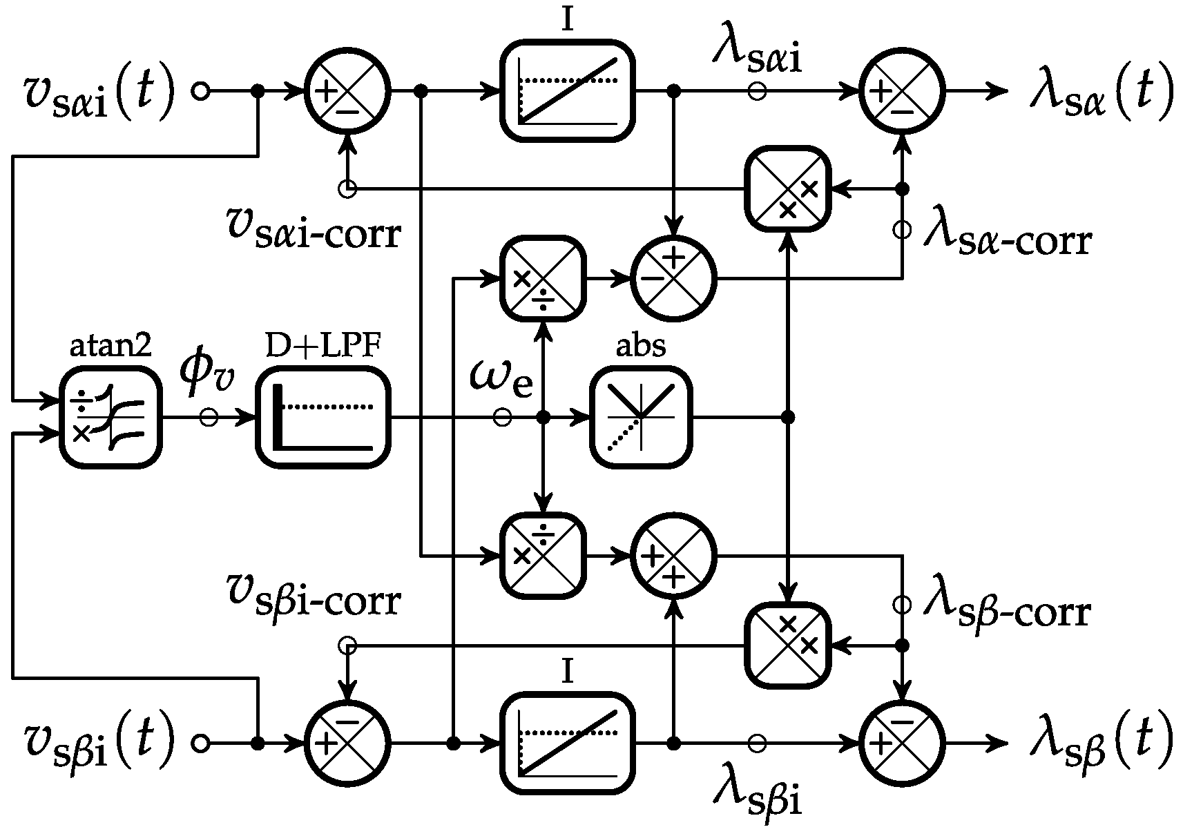
An observer of ${\theta }_{\mathrm{e}}$ and ${\omega }_{\mathrm{e}}$ for the flux-based sensorless FOC of PMSMs can therefore be constructed by combining Equations (18)–(21), as is shown by the block diagram in Figure 1.

The simplicity and filtering properties of the integrators make this observer highly desirable, especially in low-cost applications, but the integrational drift represents its major obstacle in practical implementations. The overall block diagram of the sensorless FOC is given in Figure 2 ito show how the input values of the observer from Figure 1 are obtained, and how its output values are used within the control system.

2.1. The Problem of the Integrational Drift

The integrational drift is caused by DC offsets in the direct integration voltage ($v_{\mathrm{s}\alpha \mathrm{i}}$) and the quadrature integration voltage ($v_{\mathrm{s}\beta \mathrm{i}}$), shown in Figure 1, where each DC offset is composed of two components. One component represents measurement DC offsets introduced by improperly calibrated current sensors, which in any practical implementation of the FOC must be negligibly small, while the other component represents initial conditions of the corresponding input waveform at each transient state. Since instantaneous values of ${\mathit{v}}_{\mathrm{s}\alpha \beta }$ and ${\mathit{i}}_{\mathrm{s}\alpha \beta }$ in the speed range up to the nominal speed can be observed as functions of time, they need to be expressed according to Equation (21) by rearranging it to the form

$$\begin{array}{ccc}\hfill {\int }_0^t{\omega }_{\mathrm{e}}\left(\tau \right)\mathrm{d}\tau & =& {\theta }_{\mathrm{e}}\left(t\right)+\delta ,\hfill \end{array}$$

(22)

from where ${\theta }_{\mathrm{e}}$ in steady states can be expressed as

$$\begin{array}{ccc}\hfill {\theta }_{\mathrm{e}}\left(t\right)& =& {\omega }_{\mathrm{e}}t-\delta .\hfill \end{array}$$

(23)

For the purpose of presenting the problem, it is sufficient and at the same time simpler to consider the steady state case presented by Equation (23). Hence, $v_{\mathrm{s}\alpha }$ can be expressed from Equation (6) in terms of a DC offset in $v_{\mathrm{s}\alpha }$ ($v_{\mathrm{s}\alpha ,0}$) and the magnitude of the fundamental harmonic of $v_{\mathrm{s}\alpha }$ ($v_{\mathrm{s}\alpha ,1}$) as

$$\begin{array}{ccc}\hfill v_{\mathrm{s}\alpha }\left(t\right)& =& v_{\mathrm{s}\alpha ,0}+v_{\mathrm{s}\alpha ,1}\cos ({\omega }_{\mathrm{e}}t-{\varphi }_i),\hfill \end{array}$$

(24)

and similarly, $v_{\mathrm{s}\beta }$ can be expressed in terms of a DC offset in $v_{\mathrm{s}\beta }$ ($v_{\mathrm{s}\beta ,0}$) and the magnitude of the fundamental harmonic of $v_{\mathrm{s}\beta }$ ($v_{\mathrm{s}\beta ,1}$) as

$$\begin{array}{ccc}\hfill v_{\mathrm{s}\beta }\left(t\right)& =& v_{\mathrm{s}\beta ,0}+v_{\mathrm{s}\beta ,1}\sin ({\omega }_{\mathrm{e}}t-{\varphi }_i).\hfill \end{array}$$

(25)

Based on Equation (2), $i_{\mathrm{s}\alpha }$ can be expressed in terms of a DC offset in $i_{\mathrm{s}\alpha }$ ($i_{\mathrm{s}\alpha ,0}$) and the magnitude of the fundamental harmonic of $i_{\mathrm{s}\alpha }$ ($i_{\mathrm{s}\alpha ,1}$) as

$$\begin{array}{ccc}\hfill i_{\mathrm{s}\alpha }\left(t\right)& =& i_{\mathrm{s}\alpha ,0}+i_{\mathrm{s}\alpha ,1}\cos \left({\omega }_{\mathrm{e}}t\right),\hfill \end{array}$$

(26)

while $i_{\mathrm{s}\beta }$ can be expressed in terms of a DC offset in $i_{\mathrm{s}\beta }$ ($i_{\mathrm{s}\beta ,0}$) and the magnitude of the fundamental harmonic of $i_{\mathrm{s}\beta }$ ($i_{\mathrm{s}\beta ,1}$) as

$$\begin{array}{ccc}\hfill i_{\mathrm{s}\beta }\left(t\right)& =& i_{\mathrm{s}\beta ,0}+i_{\mathrm{s}\beta ,1}\sin \left({\omega }_{\mathrm{e}}t\right).\hfill \end{array}$$

(27)

From Equation (18), based on Equations (24) and (26), $v_{\mathrm{s}\alpha \mathrm{i}}$ is expressed as

$$\begin{array}{ccc}\hfill v_{\mathrm{s}\alpha \mathrm{i}}\left(t\right)& =& v_{\mathrm{s}\alpha ,0}+v_{\mathrm{s}\alpha ,1}\cos ({\omega }_{\mathrm{e}}t-{\varphi }_i)-R_{\mathrm{s}}\left(i_{\mathrm{s}\alpha ,0}+i_{\mathrm{s}\alpha ,1}\cos \left({\omega }_{\mathrm{e}}t\right)\right),\hfill \end{array}$$

(28)

while $v_{\mathrm{s}\beta \mathrm{i}}$ is expressed from Equation (19), based on Equations (25) and (27), as

$$\begin{array}{ccc}\hfill v_{\mathrm{s}\beta \mathrm{i}}\left(t\right)& =& v_{\mathrm{s}\beta ,0}+v_{\mathrm{s}\beta ,1}\sin ({\omega }_{\mathrm{e}}t-{\varphi }_i)-R_{\mathrm{s}}\left(i_{\mathrm{s}\beta ,0}+i_{\mathrm{s}\beta ,1}\sin \left({\omega }_{\mathrm{e}}t\right)\right).\hfill \end{array}$$

(29)

After the integration of Equation (28), ${\lambda }_{\mathrm{s}\alpha }$ is obtained in the form

$$\begin{array}{ccc}\hfill {\lambda }_{\mathrm{s}\alpha }\left(t\right)& =& \frac{v_{\mathrm{s}\alpha ,1}}{{\omega }_{\mathrm{e}}}\sin ({\omega }_{\mathrm{e}}t-{\varphi }_i)-\frac{R_{\mathrm{s}}{i}_{\mathrm{s}\alpha ,1}}{{\omega }_{\mathrm{e}}}\sin \left({\omega }_{\mathrm{e}}t\right)+\left(v_{\mathrm{s}\alpha ,0}-R_{\mathrm{s}}{i}_{\mathrm{s}\alpha ,0}\right)t+{\lambda }_{\mathrm{s}\alpha }\left(0\right),\hfill \end{array}$$

(30)

while the integration of Equation (29) results in ${\lambda }_{\mathrm{s}\beta }$ in the shape

$$\begin{array}{ccc}\hfill {\lambda }_{\mathrm{s}\beta }\left(t\right)& =& -\frac{v_{\mathrm{s}\beta ,1}}{{\omega }_{\mathrm{e}}}\cos ({\omega }_{\mathrm{e}}t-{\varphi }_i)+\frac{R_{\mathrm{s}}{i}_{\mathrm{s}\beta ,1}}{{\omega }_{\mathrm{e}}}\cos \left({\omega }_{\mathrm{e}}t\right)+\left(v_{\mathrm{s}\beta ,0}-R_{\mathrm{s}}{i}_{\mathrm{s}\beta ,0}\right)t+{\lambda }_{\mathrm{s}\beta }\left(0\right).\hfill \end{array}$$

(31)

From Equations (30) and (31), it can be seen that $v_{\mathrm{s}\alpha ,0}$, $v_{\mathrm{s}\beta ,0}$, $i_{\mathrm{s}\alpha ,0}$, and $i_{\mathrm{s}\beta ,0}$ constitute the integrational drift that is initially offset by the initial conditions ${\lambda }_{\mathrm{s}\alpha }$ (0) and ${\lambda }_{\mathrm{s}\beta }$ (0).

2.2. A Solution to the Problem of the Integrational Drift

Under the assumption of a balanced three-phase power supply, $v_{\mathrm{s}\alpha ,1}=v_{\mathrm{s}\beta ,1}$ and $i_{\mathrm{s}\alpha ,1}=i_{\mathrm{s}\beta ,1}$ holds true. Following that notion, a compensation of the integrational drift can be introduced on the basis of the orthogonality between ${\lambda }_{\mathrm{s}\alpha }$ and $v_{\mathrm{s}\beta \mathrm{i}}$ as well as ${\lambda }_{\mathrm{s}\beta }$ and $v_{\mathrm{s}\alpha \mathrm{i}}$. The idea of a solution to the problem of the integrational drift can be introduced in several steps. By comparing Equation (29) with Equation (30), the correction of ${\lambda }_{\mathrm{s}\alpha }$ (${\lambda }_{\mathrm{s}\alpha -\mathrm{corr}}$) can be defined in terms of the value of ${\lambda }_{\mathrm{s}\alpha }$ directly on the output of the integrator (${\lambda }_{\mathrm{s}\alpha \mathrm{i}}$) as

$$\begin{array}{ccc}\hfill {\lambda }_{\mathrm{s}\alpha -\mathrm{corr}}\left(t\right)& =& {\lambda }_{\mathrm{s}\alpha \mathrm{i}}\left(t\right)-\frac{v_{\mathrm{s}\beta \mathrm{i}}\left(t\right)}{{\omega }_{\mathrm{e}}\left(t\right)}=\left(v_{\mathrm{s}\alpha ,0}-R_{\mathrm{s}}{i}_{\mathrm{s}\alpha ,0}\right)t+{\lambda }_{\mathrm{s}\alpha }\left(0\right)-\frac{v_{\mathrm{s}\beta ,0}-R_{\mathrm{s}}{i}_{\mathrm{s}\beta ,0}}{{\omega }_{\mathrm{e}}\left(t\right)},\hfill \end{array}$$

(32)

where ${\omega }_{\mathrm{e}}$, due to integration, is required to scale $v_{\mathrm{s}\beta \mathrm{i}}$ to the level of ${\lambda }_{\mathrm{s}\alpha }$. Since

$$\begin{array}{ccc}\hfill \left(v_{\mathrm{s}\alpha ,0}-R_{\mathrm{s}}{i}_{\mathrm{s}\alpha ,0}\right)t+{\lambda }_{\mathrm{s}\alpha }\left(0\right)& \gg & \frac{v_{\mathrm{s}\beta ,0}-R_{\mathrm{s}}{i}_{\mathrm{s}\beta ,0}}{{\omega }_{\mathrm{e}}\left(t\right)}\mathrm{for}{\omega }_{\mathrm{e}}\gg 0,\hfill \end{array}$$

(33)

and $v_{\mathrm{s}\beta ,0}$ and $i_{\mathrm{s}\beta ,0}$ are required by the FOC to be negligibly small, the integrational drift in ${\lambda }_{\mathrm{s}\alpha }$ is compensated by subtracting ${\lambda }_{\mathrm{s}\alpha -\mathrm{corr}}$ from Equation (30). Following the same reasoning, the correction of ${\lambda }_{\mathrm{s}\beta }$ (${\lambda }_{\mathrm{s}\beta -\mathrm{corr}}$) can be obtained based on Equations (28) and (31) in terms of the value of ${\lambda }_{\mathrm{s}\beta }$ directly on the output of the integrator (${\lambda }_{\mathrm{s}\beta \mathrm{i}}$) as

$$\begin{array}{ccc}\hfill {\lambda }_{\mathrm{s}\beta -\mathrm{corr}}\left(t\right)& =& {\lambda }_{\mathrm{s}\beta \mathrm{i}}\left(t\right)+\frac{v_{\mathrm{s}\alpha \mathrm{i}}\left(t\right)}{{\omega }_{\mathrm{e}}\left(t\right)}=\left(v_{\mathrm{s}\beta ,0}-R_{\mathrm{s}}{i}_{\mathrm{s}\beta ,0}\right)t+{\lambda }_{\mathrm{s}\beta }\left(0\right)+\frac{v_{\mathrm{s}\alpha ,0}-R_{\mathrm{s}}{i}_{\mathrm{s}\alpha ,0}}{{\omega }_{\mathrm{e}}\left(t\right)}.\hfill \end{array}$$

(34)

By considering

$$\begin{array}{ccc}\hfill \left(v_{\mathrm{s}\beta ,0}-R_{\mathrm{s}}{i}_{\mathrm{s}\beta ,0}\right)t+{\lambda }_{\mathrm{s}\beta }\left(0\right)& \gg & \frac{v_{\mathrm{s}\alpha ,0}-R_{\mathrm{s}}{i}_{\mathrm{s}\alpha ,0}}{{\omega }_{\mathrm{e}}\left(t\right)}\mathrm{for}{\omega }_{\mathrm{e}}\gg 0,\hfill \end{array}$$

(35)

and taking into account the requirement of the FOC for negligibly small values of $v_{\mathrm{s}\alpha ,0}$ and $i_{\mathrm{s}\alpha ,0}$, the integrational drift in ${\lambda }_{\mathrm{s}\beta }$ is compensated by subtracting ${\lambda }_{\mathrm{s}\beta -\mathrm{corr}}$ from Equation (31). Despite the compensation of the integrational drift in ${\lambda }_{\mathrm{s}\alpha }$ and ${\lambda }_{\mathrm{s}\beta }$, the integrators can still saturate. For that reason it is necessary to introduce the correction of $v_{\mathrm{s}\alpha \mathrm{i}}$ ($v_{\mathrm{s}\alpha \mathrm{i}-\mathrm{corr}}$) in the form of

$$\begin{array}{ccc}\hfill v_{\mathrm{s}\alpha \mathrm{i}-\mathrm{corr}}\left(t\right)& =& |{\omega }_{\mathrm{e}}\left(t\right)|{\lambda }_{\mathrm{s}\alpha -\mathrm{corr}}\left(t\right),\hfill \end{array}$$

(36)

which needs to be subtracted from $v_{\mathrm{s}\alpha \mathrm{i}}$, together with the correction of $v_{\mathrm{s}\beta \mathrm{i}}$($v_{\mathrm{s}\beta \mathrm{i}-\mathrm{corr}}$) that is similarly defined as

$$\begin{array}{ccc}\hfill v_{\mathrm{s}\beta \mathrm{i}-\mathrm{corr}}\left(t\right)& =& |{\omega }_{\mathrm{e}}\left(t\right)|{\lambda }_{\mathrm{s}\beta -\mathrm{corr}}\left(t\right),\hfill \end{array}$$

(37)

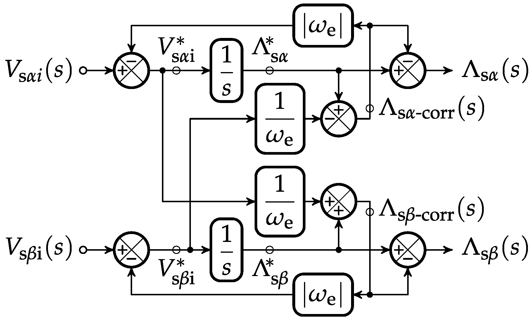
and as such needs to be subtracted from $v_{\mathrm{s}\beta \mathrm{i}}$. While the idea behind Equations (32) and (34) should be clear, the idea behind Equations (36) and (37) may not be. Thus, for an easier understanding, the proposed compensation of the integrational drift based on Equations (32)–(37) is presented in the form of the block diagram in Figure 3.

The idea behind Equation (36) can be explained by the block diagram in Figure 3 in terms of a DC offset in $v_{\mathrm{s}\alpha \mathrm{i}}$ ($v_{\mathrm{s}\alpha \mathrm{i},0}$) at $t=0$ by assuming $v_{\mathrm{s}\beta \mathrm{i}}={\lambda }_{\mathrm{s}\alpha }\left(0\right)={\lambda }_{\mathrm{s}\beta }\left(0\right)=0$, starting from $v_{\mathrm{s}\alpha \mathrm{i}}$, and making a full loop as: $v_{\mathrm{s}\alpha \mathrm{i},0}$ ⇒ $v_{\mathrm{s}\alpha \mathrm{i},0}/{\omega }_{\mathrm{e}}$ ⇒ ${\omega }_{\mathrm{e}}{v}_{\mathrm{s}\alpha \mathrm{i},0}/{\omega }_{\mathrm{e}}=v_{\mathrm{s}\alpha \mathrm{i},0}$ ⇒ $-v_{\mathrm{s}\alpha \mathrm{i},0}$ ⇒ $-v_{\mathrm{s}\alpha \mathrm{i},0}/{\omega }_{\mathrm{e}}$ ⇒ $-(-v_{\mathrm{s}\alpha \mathrm{i},0}/{\omega }_{\mathrm{e}})=v_{\mathrm{s}\alpha \mathrm{i},0}/{\omega }_{\mathrm{e}}$ ⇒ ${\omega }_{\mathrm{e}}{v}_{\mathrm{s}\alpha \mathrm{i},0}/{\omega }_{\mathrm{e}}=v_{\mathrm{s}\alpha \mathrm{i},0}$ ⇒ $-v_{\mathrm{s}\alpha \mathrm{i},0}$. As it can be seen, $v_{\mathrm{s}\alpha \mathrm{i},0}$ gets inverted and cancels itself. The idea behind Equation (37) can be explained in a similar way in terms of a DC offset in $v_{\mathrm{s}\beta \mathrm{i}}$ ($v_{\mathrm{s}\beta \mathrm{i},0}$) at $t=0$ by assuming $v_{\mathrm{s}\alpha \mathrm{i}}={\lambda }_{\mathrm{s}\alpha }\left(0\right)={\lambda }_{\mathrm{s}\beta }\left(0\right)=0$ and starting from $v_{\mathrm{s}\beta \mathrm{i}}$ as: $v_{\mathrm{s}\beta \mathrm{i},0}$ ⇒ $v_{\mathrm{s}\beta \mathrm{i},0}/{\omega }_{\mathrm{e}}$ ⇒ $-v_{\mathrm{s}\beta \mathrm{i},0}/{\omega }_{\mathrm{e}}$ ⇒ $-{\omega }_{\mathrm{e}}{v}_{\mathrm{s}\beta \mathrm{i},0}/{\omega }_{\mathrm{e}}=-v_{\mathrm{s}\beta \mathrm{i},0}$ ⇒ $-(-v_{\mathrm{s}\beta \mathrm{i},0})=v_{\mathrm{s}\beta \mathrm{i},0}$ ⇒ $v_{\mathrm{s}\beta \mathrm{i},0}/{\omega }_{\mathrm{e}}$ ⇒ ${\omega }_{\mathrm{e}}{v}_{\mathrm{s}\beta \mathrm{i},0}/{\omega }_{\mathrm{e}}=v_{\mathrm{s}\beta \mathrm{i},0}$ ⇒ $-v_{\mathrm{s}\beta \mathrm{i},0}$. As expected, $v_{\mathrm{s}\beta \mathrm{i},0}$ gets inverted as well and cancels itself. Therefore, Equations (32)–(37) constitute the proposed compensation of the integrational drift that, besides the effects of integration, does not have any additional influence on the amplitude nor the phase of the fundamental harmonic of ${\lambda }_{\mathrm{s}\alpha }$ and ${\lambda }_{\mathrm{s}\beta }$ in steady states, if the assumption of a balanced three-phase power supply holds true.

2.3. A Characterization of the Proposed Compensation

From the definition of the problem presented by Equations (28)–(31), it is clear that the proposed compensation of the integrational drift completely eliminates the integrational drift in steady states without affecting the amplitude nor the phase of ${\lambda }_{\mathrm{s}\alpha }$ and ${\lambda }_{\mathrm{s}\beta }$. To avoid causality-related problems that might arise depending on the implementation, ${\omega }_{\mathrm{e}}$ can be precalculated by substituting the phase angle of ${\mathit{v}}_{\mathrm{s}\alpha \beta }$ (${\varphi }_v$) that can be obtained from the instantaneous values of $v_{\mathrm{s}\alpha \mathrm{i}}$ and $v_{\mathrm{s}\beta \mathrm{i}}$ as

$$\begin{array}{ccc}\hfill {\varphi }_v\left(t\right)& =& \mathrm{atan}2(v_{\mathrm{s}\beta \mathrm{i}}\left(t\right),v_{\mathrm{s}\alpha \mathrm{i}}\left(t\right)),\hfill \end{array}$$

(38)

instead of ${\theta }_{\mathrm{e}}$ in Equation (21), as is shown in Figure 3.

The equivalent steady state representation of the system in Figure 3 in the Laplace domain is shown in Figure 4 in the form of the block diagram that can be used for a characterization of the proposed compensation. The system in Figure 4 can be algebraically described by the following equations:

$$\begin{array}{ccc}\hfill {\Lambda }_{\mathrm{s}\alpha }\left(s\right)& =& {\Lambda }_{\mathrm{s}\alpha }^{*}\left(s\right)-{\Lambda }_{\mathrm{s}\alpha -\mathrm{corr}}\left(s\right),\hfill \end{array}$$

(39)

$$\begin{array}{ccc}\hfill {\Lambda }_{\mathrm{s}\beta }\left(s\right)& =& {\Lambda }_{\mathrm{s}\beta }^{*}\left(s\right)-{\Lambda }_{\mathrm{s}\beta -\mathrm{corr}}\left(s\right),\hfill \end{array}$$

(40)

$$\begin{array}{ccc}\hfill {\Lambda }_{\mathrm{s}\alpha }^{*}\left(s\right)& =& \frac{V_{\mathrm{s}\alpha \mathrm{i}}^{*}\left(s\right)}{s},\hfill \end{array}$$

(41)

$$\begin{array}{ccc}\hfill {\Lambda }_{\mathrm{s}\beta }^{*}\left(s\right)& =& \frac{V_{\mathrm{s}\beta \mathrm{i}}^{*}\left(s\right)}{s},\hfill \end{array}$$

(42)

$$\begin{array}{ccc}\hfill {\Lambda }_{\mathrm{s}\alpha -\mathrm{corr}}\left(s\right)& =& {\Lambda }_{\mathrm{s}\alpha }^{*}\left(s\right)-\frac{V_{\mathrm{s}\beta \mathrm{i}}^{*}\left(s\right)}{{\omega }_{\mathrm{e}}},\hfill \end{array}$$

(43)

$$\begin{array}{ccc}\hfill {\Lambda }_{\mathrm{s}\beta -\mathrm{corr}}\left(s\right)& =& {\Lambda }_{\mathrm{s}\beta }^{*}\left(s\right)+\frac{V_{\mathrm{s}\alpha \mathrm{i}}^{*}\left(s\right)}{{\omega }_{\mathrm{e}}},\hfill \end{array}$$

(44)

$$\begin{array}{ccc}\hfill V_{\mathrm{s}\alpha \mathrm{i}}^{*}\left(s\right)& =& V_{\mathrm{s}\alpha \mathrm{i}}\left(s\right)-\left|{\omega }_{\mathrm{e}}\right|{\Lambda }_{\mathrm{s}\alpha -\mathrm{corr}}\left(s\right),\mathrm{and}\hfill \end{array}$$

(45)

$$\begin{array}{ccc}\hfill V_{\mathrm{s}\beta \mathrm{i}}^{*}\left(s\right)& =& V_{\mathrm{s}\beta \mathrm{i}}\left(s\right)-\left|{\omega }_{\mathrm{e}}\right|{\Lambda }_{\mathrm{s}\beta -\mathrm{corr}}\left(s\right),\hfill \end{array}$$

(46)

which can be combined into the closed-loop system

$$\begin{array}{ccc}\hfill \left[\begin{array}{c}{\Lambda }_{\mathrm{s}\alpha }\left(s\right)\\ {\Lambda }_{\mathrm{s}\beta }\left(s\right)\end{array}\right]& =& \frac{s}{2|{\omega }_{\mathrm{e}}|s^2+2{\omega }_{\mathrm{e}}^{2}s+\left|{\omega }_{\mathrm{e}}^3\right|}\left[\begin{array}{cc}-s& \mathrm{sgn}\left({\omega }_{\mathrm{e}}\right)\left(s+|{\omega }_{\mathrm{e}}|\right)\\ -\mathrm{sgn}\left({\omega }_{\mathrm{e}}\right)\left(s+|{\omega }_{\mathrm{e}}|\right)& -s\end{array}\right]\left[\begin{array}{c}{V}_{\mathrm{s}\alpha \mathrm{i}}\left(s\right)\\ V_{\mathrm{s}\beta \mathrm{i}}\left(s\right)\end{array}\right]\hfill \end{array}$$

(47)

that relates each of the two outputs to the two inputs of the system.

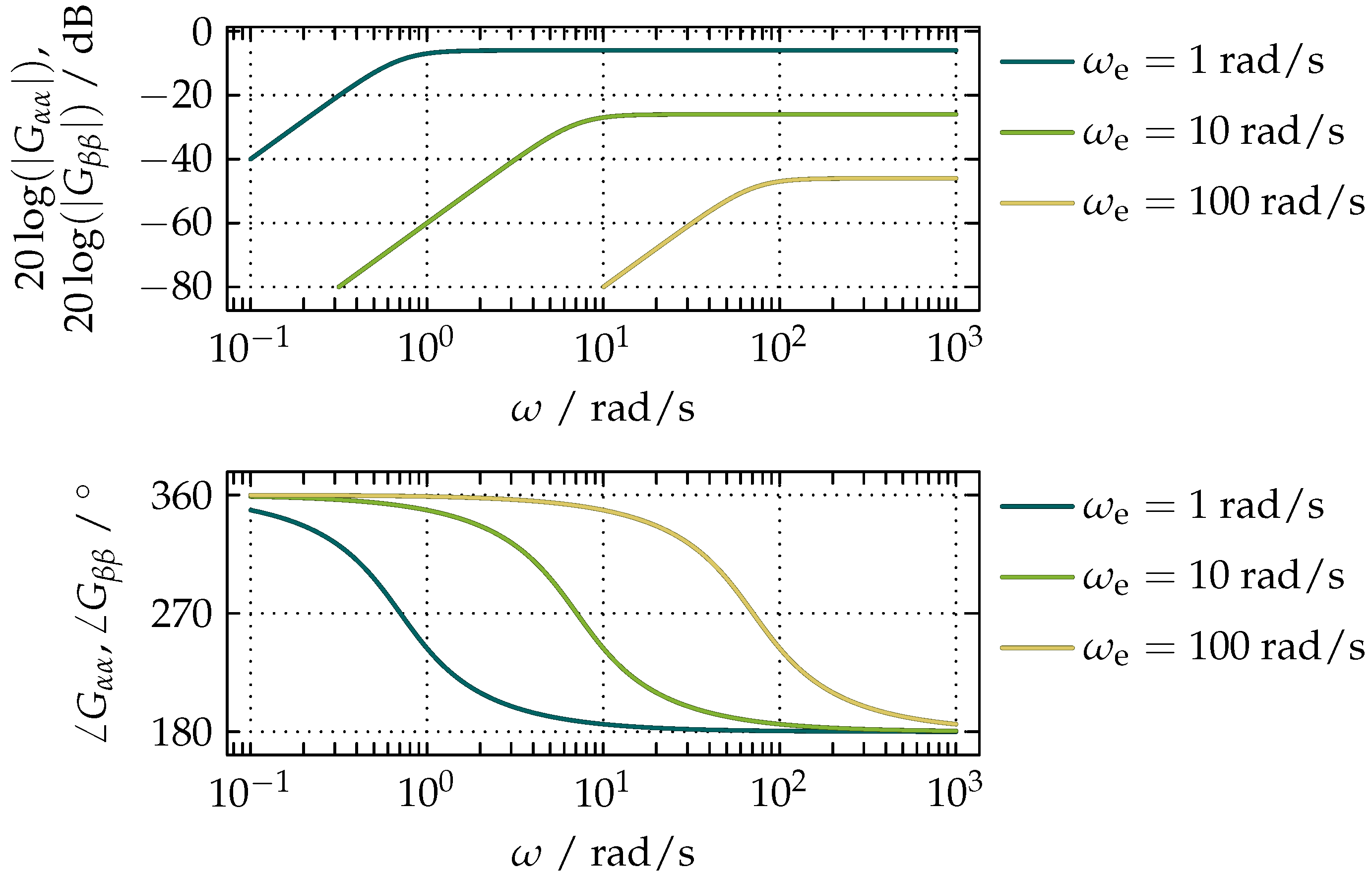
The frequency response of each output in relation to the corresponding input can be obtained by observing the system as multiple single input–single output systems, where each output is described by the corresponding transfer function with the observed input. Since the transfer function between ${\Lambda }_{\mathrm{s}\alpha }$ and $V_{\mathrm{s}\alpha \mathrm{i}}$ according to Equation (47) is identical to the transfer function between ${\Lambda }_{\mathrm{s}\beta }$ and $V_{\mathrm{s}\beta \mathrm{i}}$, that is

$$\begin{array}{ccc}\hfill G_{\alpha \alpha }\left(s\right)& =& \frac{{\Lambda }_{\mathrm{s}\alpha }\left(s\right)}{V_{\mathrm{s}\alpha \mathrm{i}}\left(s\right)}=G_{\beta \beta }\left(s\right)=\frac{{\Lambda }_{\mathrm{s}\beta }\left(s\right)}{V_{\mathrm{s}\beta \mathrm{i}}\left(s\right)}=\frac{-s^2}{2|{\omega }_{\mathrm{e}}|s^2+2{\omega }_{\mathrm{e}}^{2}s+\left|{\omega }_{\mathrm{e}}^3\right|},\hfill \end{array}$$

(48)

they share the same Bode plots shown in Figure 5 whose characteristic represents an adaptive second-order HPF with the cut-off frequency and the gain determined by the value of ${\omega }_{\mathrm{e}}$, and the added phase shift of ${180}^{\circ }$ in comparison to the standard second-order HPF.

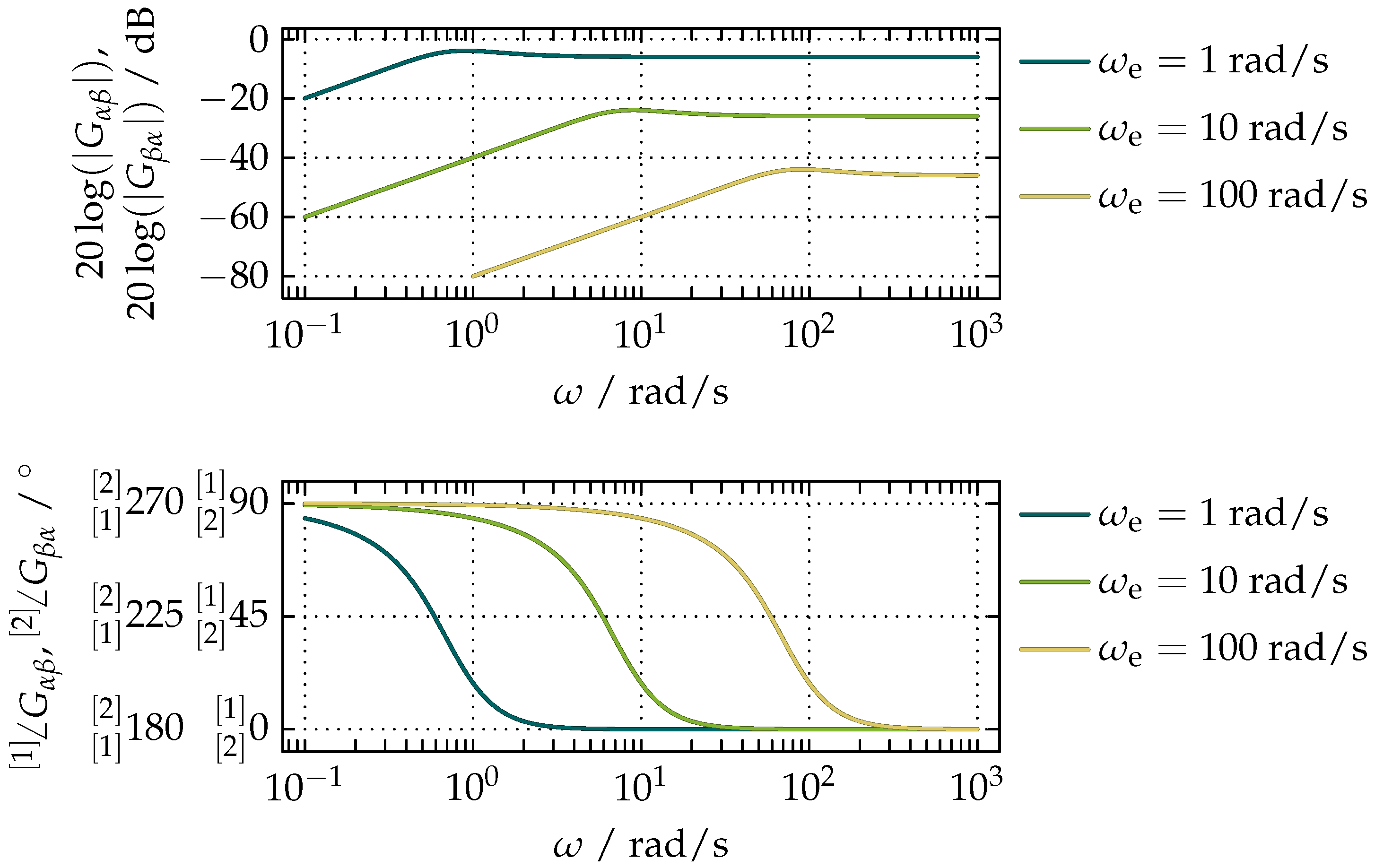
Analogously, the transfer function between ${\Lambda }_{\mathrm{s}\alpha }$ and $V_{\mathrm{s}\beta \mathrm{i}}$ is

$$\begin{array}{ccc}\hfill G_{\alpha \beta }\left(s\right)& =& \frac{{\Lambda }_{\mathrm{s}\alpha }\left(s\right)}{V_{\mathrm{s}\beta \mathrm{i}}\left(s\right)}=\frac{\mathrm{sgn}\left({\omega }_{\mathrm{e}}\right)\left(s+|{\omega }_{\mathrm{e}}|\right)}{2|{\omega }_{\mathrm{e}}|s^2+2{\omega }_{\mathrm{e}}^{2}s+\left|{\omega }_{\mathrm{e}}^3\right|},\hfill \end{array}$$

(49)

while the transfer function between ${\Lambda }_{\mathrm{s}\beta }$ and $V_{\mathrm{s}\alpha \mathrm{i}}$ is

$$\begin{array}{ccc}\hfill G_{\beta \alpha }\left(s\right)& =& \frac{{\Lambda }_{\mathrm{s}\beta }\left(s\right)}{V_{\mathrm{s}\alpha \mathrm{i}}\left(s\right)}=\frac{-\mathrm{sgn}\left({\omega }_{\mathrm{e}}\right)\left(s+|{\omega }_{\mathrm{e}}|\right)}{2|{\omega }_{\mathrm{e}}|s^2+2{\omega }_{\mathrm{e}}^{2}s+\left|{\omega }_{\mathrm{e}}^3\right|}.\hfill \end{array}$$

(50)

The common Bode plots of $G_{\alpha \beta }$ and $G_{\beta \alpha }$ are shown in Figure 6.

They show that the frequency response of each output in relation to the opposite input resembles the standard first-order HPF with a small rise just below the cut-off frequency, which is also the gain determined by the value of ${\omega }_{\mathrm{e}}$. The only difference between the two transfer functions can be seen in the phase plot as the extra ${180}^{\circ }$ phase shift whose sign is determined by the sign of ${\omega }_{\mathrm{e}}$.

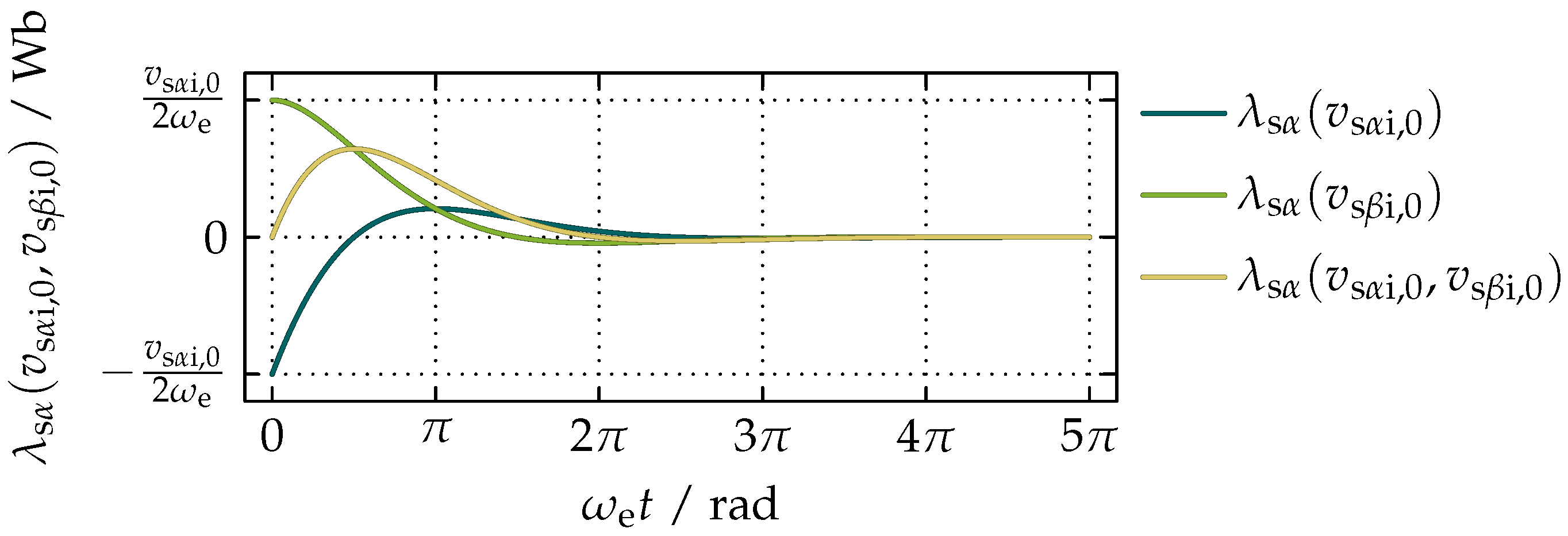
Transient states in the system caused by the integrational drift can be analyzed in the time domain by multiplying each of the transfer functions by the Laplace transform of the unit step function, taking the inverse Laplace transform of their product, and adding up the orthogonal components of the same output. Thus, the component of the integrational drift in ${\lambda }_{\mathrm{s}\alpha }$ imposed by $v_{\mathrm{s}\alpha \mathrm{i},0}$ in the form of the step function, that is $v_{\mathrm{s}\alpha \mathrm{i},0}\ne 0$ and constant for $t\ge 0$ and ${\omega }_{\mathrm{e}}>0$ is

$$\begin{array}{ccc}\hfill {\lambda }_{\mathrm{s}\alpha }(v_{\mathrm{s}\alpha \mathrm{i},0}\left(t\right),t)& =& v_{\mathrm{s}\alpha \mathrm{i},0}\left(t\right){\mathcal{L}}^{-1}\left\{\frac{1}{s}{G}_{\alpha \alpha }\left(s\right)\right\}\left(t\right)=\frac{v_{\mathrm{s}\alpha \mathrm{i},0}\left(t\right)}{\sqrt{2}{\omega }_{\mathrm{e}}}\sin \left(\frac{{\omega }_{\mathrm{e}}t}{2}-\frac{\pi }{4}\right)\exp \left(-\frac{{\omega }_{\mathrm{e}}t}{2}\right).\hfill \end{array}$$

(51)

The integrational drift imposed by $v_{\mathrm{s}\beta \mathrm{i},0}$, for $v_{\mathrm{s}\alpha \mathrm{i},0}\ne 0$ and constant for $t\ge 0$, on ${\lambda }_{\mathrm{s}\alpha }$ for ${\omega }_{\mathrm{e}}>0$ is

$$\begin{array}{ccc}\hfill {\lambda }_{\mathrm{s}\alpha }(v_{\mathrm{s}\beta \mathrm{i},0}\left(t\right),t)& =& v_{\mathrm{s}\beta \mathrm{i},0}\left(t\right){\mathcal{L}}^{-1}\left\{\frac{1}{s}{G}_{\alpha \beta }\left(s\right)\right\}\left(t\right)=\frac{v_{\mathrm{s}\beta \mathrm{i},0}\left(t\right)}{\sqrt{2}{\omega }_{\mathrm{e}}}\sin \left(\frac{{\omega }_{\mathrm{e}}t}{2}+\frac{\pi }{4}\right)\exp \left(-\frac{{\omega }_{\mathrm{e}}t}{2}\right).\hfill \end{array}$$

(52)

Based on Equations (51) and (52), the total integrational drift in ${\lambda }_{\mathrm{s}\alpha }$ is defined as

$$\begin{array}{ccc}\hfill {\lambda }_{\mathrm{s}\alpha }(v_{\mathrm{s}\alpha \mathrm{i},0}\left(t\right),v_{\mathrm{s}\beta \mathrm{i},0}\left(t\right),t)& =& {\lambda }_{\mathrm{s}\alpha }(v_{\mathrm{s}\alpha \mathrm{i},0}\left(t\right),t)+{\lambda }_{\mathrm{s}\alpha }(v_{\mathrm{s}\beta \mathrm{i},0}\left(t\right),t)\hfill \end{array}$$

(53)

and graphically presented in the plot in Figure 7.

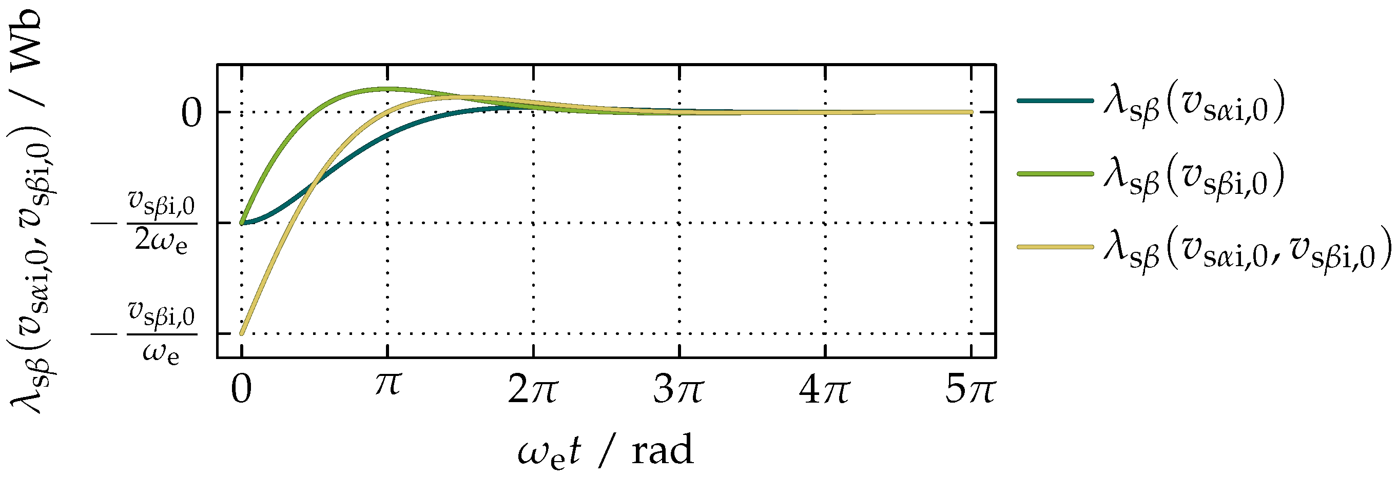
Equivalently, the component of the integrational drift in ${\lambda }_{\mathrm{s}\beta }$ imposed by $v_{\mathrm{s}\beta \mathrm{i},0}$ in the form of the step function, that is $v_{\mathrm{s}\beta \mathrm{i},0}\ne 0$ and constant for $t\ge 0$ and ${\omega }_{\mathrm{e}}>0$ is obtained in the form

$$\begin{array}{ccc}\hfill {\lambda }_{\mathrm{s}\beta }(v_{\mathrm{s}\beta \mathrm{i},0}\left(t\right),t)& =& v_{\mathrm{s}\beta \mathrm{i},0}\left(t\right){\mathcal{L}}^{-1}\left\{\frac{1}{s}{G}_{\beta \beta }\left(s\right)\right\}\left(t\right)=\frac{v_{\mathrm{s}\beta \mathrm{i},0}\left(t\right)}{\sqrt{2}{\omega }_{\mathrm{e}}}\sin \left(\frac{{\omega }_{\mathrm{e}}t}{2}-\frac{\pi }{4}\right)\exp \left(-\frac{{\omega }_{\mathrm{e}}t}{2}\right),\hfill \end{array}$$

(54)

while the integrational drift imposed by $v_{\mathrm{s}\alpha \mathrm{i},0}$ on ${\lambda }_{\mathrm{s}\beta }$, for $v_{\mathrm{s}\alpha \mathrm{i},0}\ne 0$ and constant for $t\ge 0$, is

$$\begin{array}{ccc}\hfill {\lambda }_{\mathrm{s}\beta }(v_{\mathrm{s}\alpha \mathrm{i},0}\left(t\right),t)& =& v_{\mathrm{s}\alpha \mathrm{i},0}\left(t\right){\mathcal{L}}^{-1}\left\{\frac{1}{s}{G}_{\beta \alpha }\left(s\right)\right\}\left(t\right)=-\frac{v_{\mathrm{s}\alpha \mathrm{i},0}\left(t\right)}{\sqrt{2}{\omega }_{\mathrm{e}}}\sin \left(\frac{{\omega }_{\mathrm{e}}t}{2}+\frac{\pi }{4}\right)\exp \left(-\frac{{\omega }_{\mathrm{e}}t}{2}\right).\hfill \end{array}$$

(55)

Based on Equations (54) and (55), the total integrational drift in ${\lambda }_{\mathrm{s}\beta }$ is expressed as

$$\begin{array}{ccc}\hfill {\lambda }_{\mathrm{s}\beta }(v_{\mathrm{s}\alpha \mathrm{i},0}\left(t\right),v_{\mathrm{s}\beta \mathrm{i},0}\left(t\right),t)& =& {\lambda }_{\mathrm{s}\beta }(v_{\mathrm{s}\beta \mathrm{i},0}\left(t\right),t)+{\lambda }_{\mathrm{s}\beta }(v_{\mathrm{s}\alpha \mathrm{i},0}\left(t\right),t)\hfill \end{array}$$

(56)

and graphically presented in the plot in Figure 8.

The relative scaling of the axes in Figure 7 and Figure 8 show that the duration of each transient state of the proposed compensation of the integrational drift is inversely proportional to ${\omega }_{\mathrm{e}}$. The exponential function $\exp (-{\omega }_{\mathrm{e}}t/2)$ in Equations (51), (52), (54), and (55) determines the duration of each transient state and therefore ensures that a minimum of 95.68% of the integrational drift introduced by $v_{\mathrm{s}\alpha \mathrm{i},0}$ and $v_{\mathrm{s}\beta \mathrm{i},0}$ is filtered out from ${\lambda }_{\mathrm{s}\alpha }$ and ${\lambda }_{\mathrm{s}\beta }$ already after the first electrical period of the observed transient state.

3. Simulation Results of the Proposed Compensation

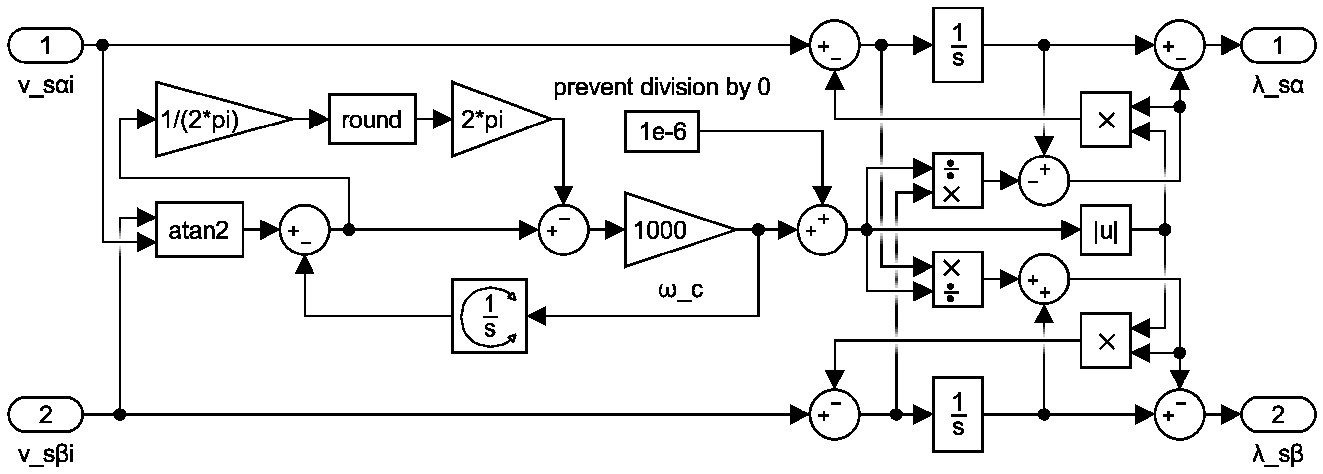
Two simulations of the proposed compensation of the integrational drift, without the rest of the control system and direct relations to possible states of the drive, were made in MATLAB Simulink using the block diagram shown in Figure 9 to demonstrate its overall performance as well as to avoid the analytical derivation of the response for sinusoidal waveforms.

In Figure 9, the derivative of ${\varphi }_v$ filtered by an LPF represented by the $\mathrm{D}+\mathrm{LPF}$ block in Figure 9 is implemented in terms of an integrator and the cut-off frequency of the LPF for filtering ${\omega }_{\mathrm{e}}$ (${\omega }_{\mathrm{c}}$) based on the transfer function

$$\begin{array}{ccc}\hfill G_{\mathrm{D}+\mathrm{LPF}}\left(s\right)& =& s\frac{{\omega }_{\mathrm{c}}}{s+{\omega }_{\mathrm{c}}}=\frac{{\omega }_{\mathrm{c}}s}{s+{\omega }_{\mathrm{c}}}=\frac{{\omega }_{\mathrm{c}}}{{\displaystyle 1+\frac{{\omega }_{\mathrm{c}}\phantom{(}}{s}}}.\hfill \end{array}$$

(57)

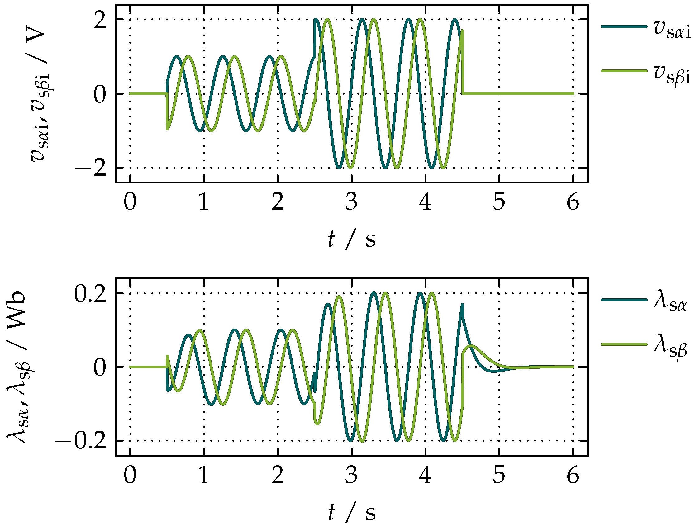
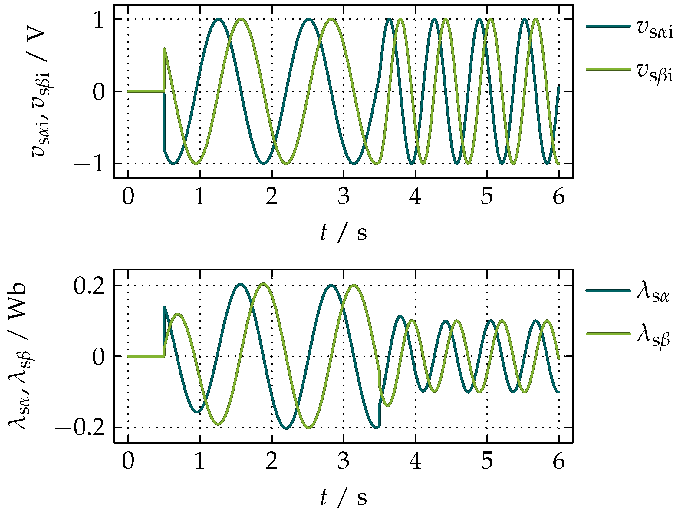
Since the $\mathrm{atan}2$ block gives values in the range from $-\pi$ to $\pi$ inclusive, the output angle of the integrator is wrapped to the same range as well as the resulting error signal via the $[1/(2\pi )\Rightarrow \mathrm{round}\Rightarrow 2\pi ]$ branch. To prevent the case of division by 0, a negligibly small value ${10}^{-6}$ is added to ${\omega }_{\mathrm{e}}$. The results of the first simulation presented in Figure 10 show sudden steps in the amplitudes of $v_{\mathrm{s}\alpha \mathrm{i}}$ and $v_{\mathrm{s}\beta \mathrm{i}}$ with the resulting waveforms of ${\lambda }_{\mathrm{s}\alpha }$ and ${\lambda }_{\mathrm{s}\beta }$ at the constant value of ${\omega }_{\mathrm{e}}$ of $10\mathrm{rad}/\mathrm{s}$.

The decaying transients visible from the time of 4.5 s onward when $v_{\mathrm{s}\alpha \mathrm{i}}$ and $v_{\mathrm{s}\beta \mathrm{i}}$ drop to zero are essentially the transients in ${\lambda }_{\mathrm{s}\alpha }$ and ${\lambda }_{\mathrm{s}\beta }$ presented in Figure 7 and Figure 8. The results of the second simulation presented in Figure 11 show a step in ${\omega }_{\mathrm{e}}$ from $5\mathrm{rad}/\mathrm{s}$ to $10\mathrm{rad}/\mathrm{s}$, where the amplitudes of $v_{\mathrm{s}\alpha \mathrm{i}}$ and $v_{\mathrm{s}\beta \mathrm{i}}$ after the initial time of 0.5 s are kept constant.

In Figure 10 and Figure 11, the sudden changes in ${\lambda }_{\mathrm{s}\alpha }$ and ${\lambda }_{\mathrm{s}\beta }$ are imposed by Equations (32) and (34), while the remaining transients are introduced by the corrections described by Equations (36) and (37).

A Comparison of the Proposed Compensation with Referred Methods

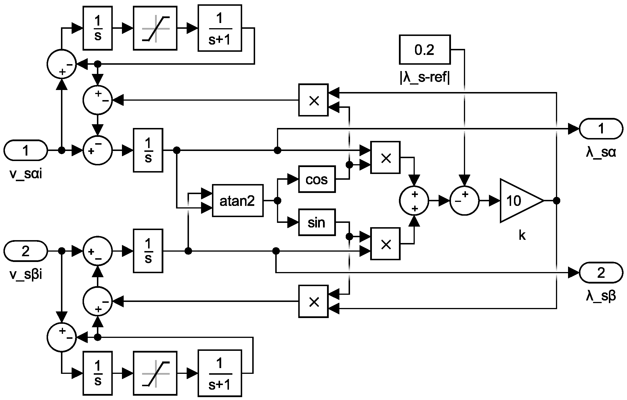
For the purpose of a qualitative comparison of the proposed method with the state of the art, two methods were selected. The first method is the method common to [18,19] presented by the block diagram in Figure 12. The second method represents the standard method with LPFs presented in [3,4,5,6,7,8], where the integrators in Figure 1 are replaced by LPFs.

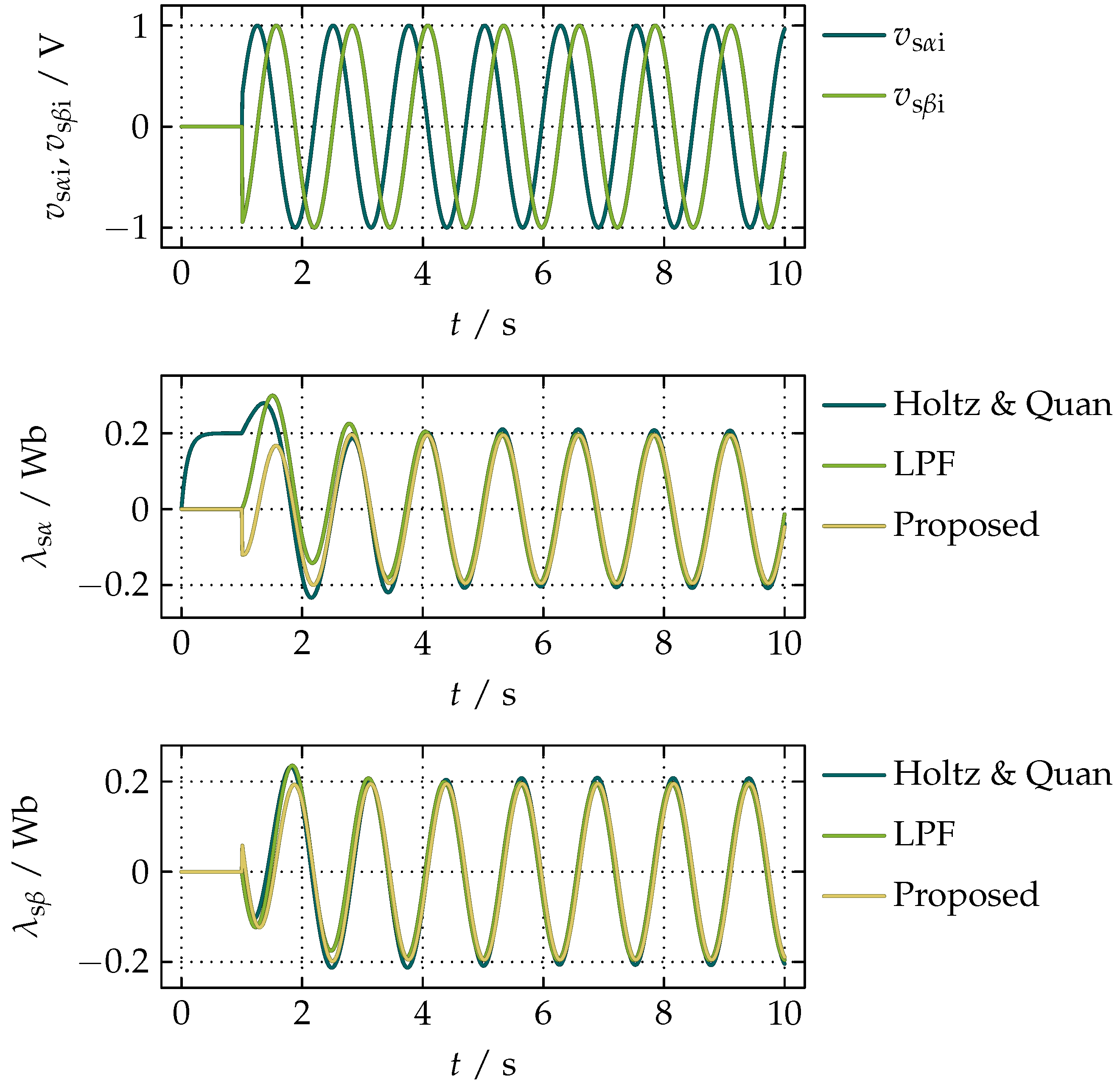
The results of a parallel simulation of the three methods for a sudden step in the amplitudes of $v_{\mathrm{s}\alpha \mathrm{i}}$ and $v_{\mathrm{s}\beta \mathrm{i}}$ at $5\mathrm{rad}/\mathrm{s}$ are presented in Figure 13.

From the results presented in Figure 13, it can be seen that the proposed compensation has the fastest response. The dynamics of the method by Holtz and Quan can be adjusted by the k block, where higher values give faster response but introduce a phase shift in the resulting waveforms of ${\lambda }_{\mathrm{s}\alpha }$ and ${\lambda }_{\mathrm{s}\beta }$. The LPFs serve for filtering of the estimated integrational drift that can be limited by the saturation blocks. The downside of the method by Holtz and Quan is the requirement of the reference value of the magnitude of the stator magnetic flux linkage. The dynamics of the method with LPFs is completely determined by the cut-off frequencies of the filters that also influence the amplitudes of ${\lambda }_{\mathrm{s}\alpha }$ and ${\lambda }_{\mathrm{s}\beta }$, and a certain phase shift always exists if it is not adequately compensated.

4. Experiment Results of the Sensorless FOC with the Proposed Compensation

The proposed compensation of the integrational drift was implemented as a part of the observer presented in Figure 1 on a Texas Instruments TMS320F28335 digital signal processor (DSP) and successfully tested on a motor whose parameters are given in

Table 1. Parameters of the test motor.

Parameter	Symbol	Value	Unit
DC-Link Voltage	$v_{\mathrm{DC}}$	24.00	V
Nominal Speed	$n_{\mathrm{n}}$	4.15	krpm
Nominal Torque	$T_{\mathrm{n}}$	0.36	Nm
Number of Pole Pairs	$p_{\mathrm{p}}$	2.00
Stator Resistance	$R_{\mathrm{s}}$	0.11	$\mathsf{\Omega }$
Direct Synchronous Inductance	$L_{\mathrm{d}}$	0.27	mH
Quadrature Synchronous Inductance	$L_{\mathrm{q}}$	0.39	mH
Rotor Flux Linkage Constant	${\lambda }_{\mathrm{m}}$	13.59	mWb

.

The test motor was chosen based on its relatively small size and thereby small mechanical time constant that makes it highly dynamic. The sensorless FOC of such motors is generally difficult, especially without any load in the low speed range.

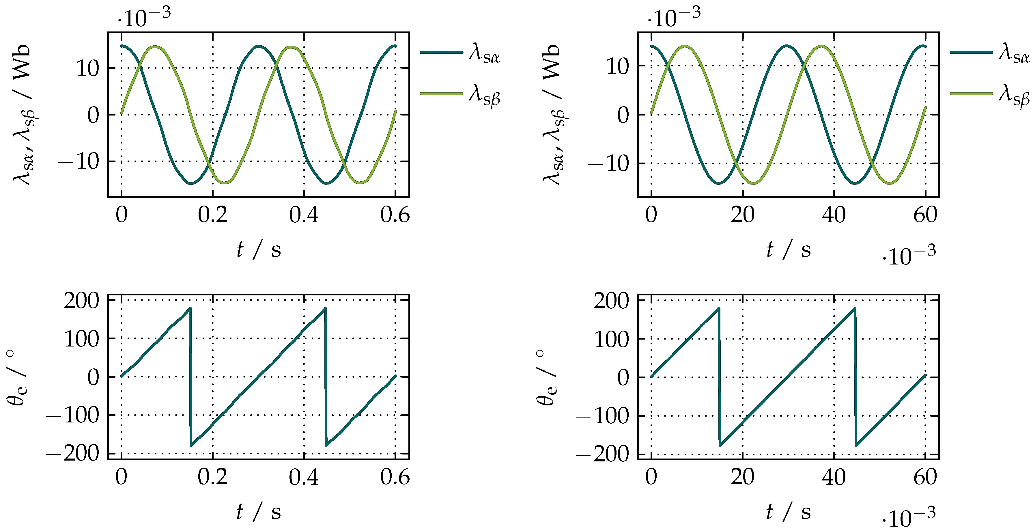
The top plots in Figure 14 show the estimated waveforms of ${\lambda }_{\mathrm{s}\alpha }$ and ${\lambda }_{\mathrm{s}\beta }$ obtained without any load at $100\mathrm{rpm}$ (left) and $1000\mathrm{rpm}$ (right), wherein the bottom plots show the corresponding estimated values of ${\theta }_{\mathrm{e}}$.

Instead of comparing ${\theta }_{\mathrm{e}}$ with the actual electrical angular position of the rotor (${\theta }_{\mathrm{e}-\mathrm{act}}$) obtained by the encoder, the performance of the proposed compensation of the integrational drift can be observed more conveniently via the error in ${\theta }_{\mathrm{e}}$ (${\theta }_{\mathrm{e}-\mathrm{err}}$) defined as

$$\begin{array}{ccc}\hfill {\theta }_{\mathrm{e}-\mathrm{err}}\left(t\right)& =& {\theta }_{\mathrm{e}-\mathrm{act}}\left(t\right)-{\theta }_{\mathrm{e}}\left(t\right).\hfill \end{array}$$

(58)

Besides ${\theta }_{\mathrm{e}-\mathrm{err}}$, for presenting measurement results, it is also convenient to show the actual speed of the rotor ($n_{\mathrm{act}}$). Since $n_{\mathrm{act}}$ is typically expressed in $\mathrm{rpm}$, the estimated counterpart of $n_{\mathrm{act}}$ (n) is obtained in terms of the number of pole pairs ($p_{\mathrm{p}}$) and ${\omega }_{\mathrm{e}}$ as

$$\begin{array}{ccc}\hfill n\left(t\right)& =& \frac{60}{2\pi p_{\mathrm{p}}}{\omega }_{\mathrm{e}}\left(t\right).\hfill \end{array}$$

(59)

The major issue in practical applications of sensorless algorithms that do not utilize a high frequency current injection with a heterodyne filtering technique is the startup process which requires the knowledge of the spatial angular position of the rotor magnetic field. This is especially true in the case of PMSMs whose rotor magnetic field, in contrast to SCIMs, is spatially fixed to the mechanical angular position of the rotor. A startup is typically performed by aligning the direct axis of the rotor with the magnetic axis of the phase A and then injecting a certain value of the current in the direction of the quadrature axis of the rotor, while slowly increasing ${\theta }_{\mathrm{e}}$ in the form of the ramp function. That way, the rotor is spun up to a certain speed at which the sensorless algorithm takes over. The first problem with this approach is that the value of the current is unknown and dependent on the load. If the current is set to its nominal value, the induced magnetic field is usually misaligned with the direct axis of the rotor, which results in a reduced value of the electromagnetic torque ($T_{\mathrm{em}}$). The second problem is the speed of acceleration that should not be too fast so that the rotor does not lose synchronism. The third problem is the transition between the startup and the sensorless algorithm, which due to the differences in ${\theta }_{\mathrm{e}}$ and the amplitude of the current is often noticeable.

The proposed compensation of the integrational drift enables nearly a smooth startup from a standstill, as shown in Figure 15, while in the case of the loaded motor, the startup from a standstill is rather abrupt, but still possible, as can be seen in Figure 16.

The plots on the left side of Figure 15 show the values of $n_{\mathrm{act}}$ and n obtained during the acceleration from $0\mathrm{rpm}$ to $4000\mathrm{rpm}$ within 1 s, while the plots on the right side show the values for an equivalent acceleration within the time-span of 10 s. From the presented data, it can be seen that the noise in n caused by the higher initial values of ${\theta }_{\mathrm{e}-\mathrm{err}}$ has little influence on $n_{\mathrm{act}}$ due to the inertia of the rotor. In addition, ${\theta }_{\mathrm{e}-\mathrm{err}}$ shows that the uncertainty of the actual angular position of the rotor practically vanishes within 0.5 s. Figure 16 presents the measurement data of the reference speed of the rotor ($n_{\mathrm{ref}}$), $n_{\mathrm{act}}$, n, $T_{\mathrm{em}}$, and ${\theta }_{\mathrm{e}-\mathrm{err}}$, during the linear acceleration from $0\mathrm{rpm}$ to $2000\mathrm{rpm}$ under the load torque of 90% of the nominal torque ($T_{\mathrm{n}}$) as well as the intermittent periodic loading at $2000\mathrm{rpm}$. While the first and third plots show the same variables presented in Figure 15, the second plot shows $T_{\mathrm{em}}$ calculated based on $i_{\mathrm{sq}}$ as

$$\begin{array}{ccc}\hfill T_{\mathrm{em}}\left(t\right){|}_{i_{\mathrm{sd}}\left(t\right)=0}& =& \frac{3}{2}{p}_{\mathrm{p}}{\lambda }_{\mathrm{m}}{i}_{\mathrm{sq}}\left(t\right).\hfill \end{array}$$

(60)

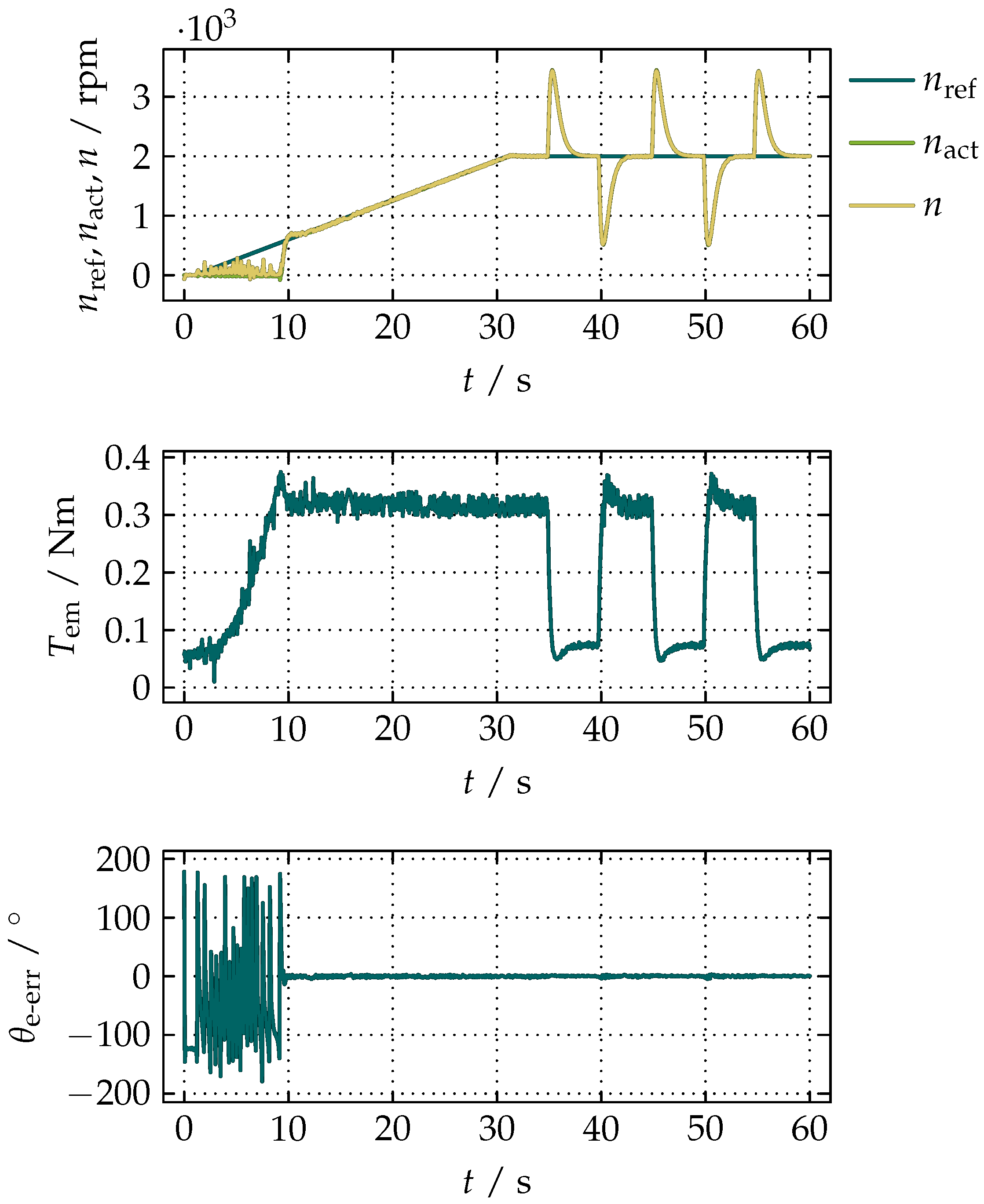
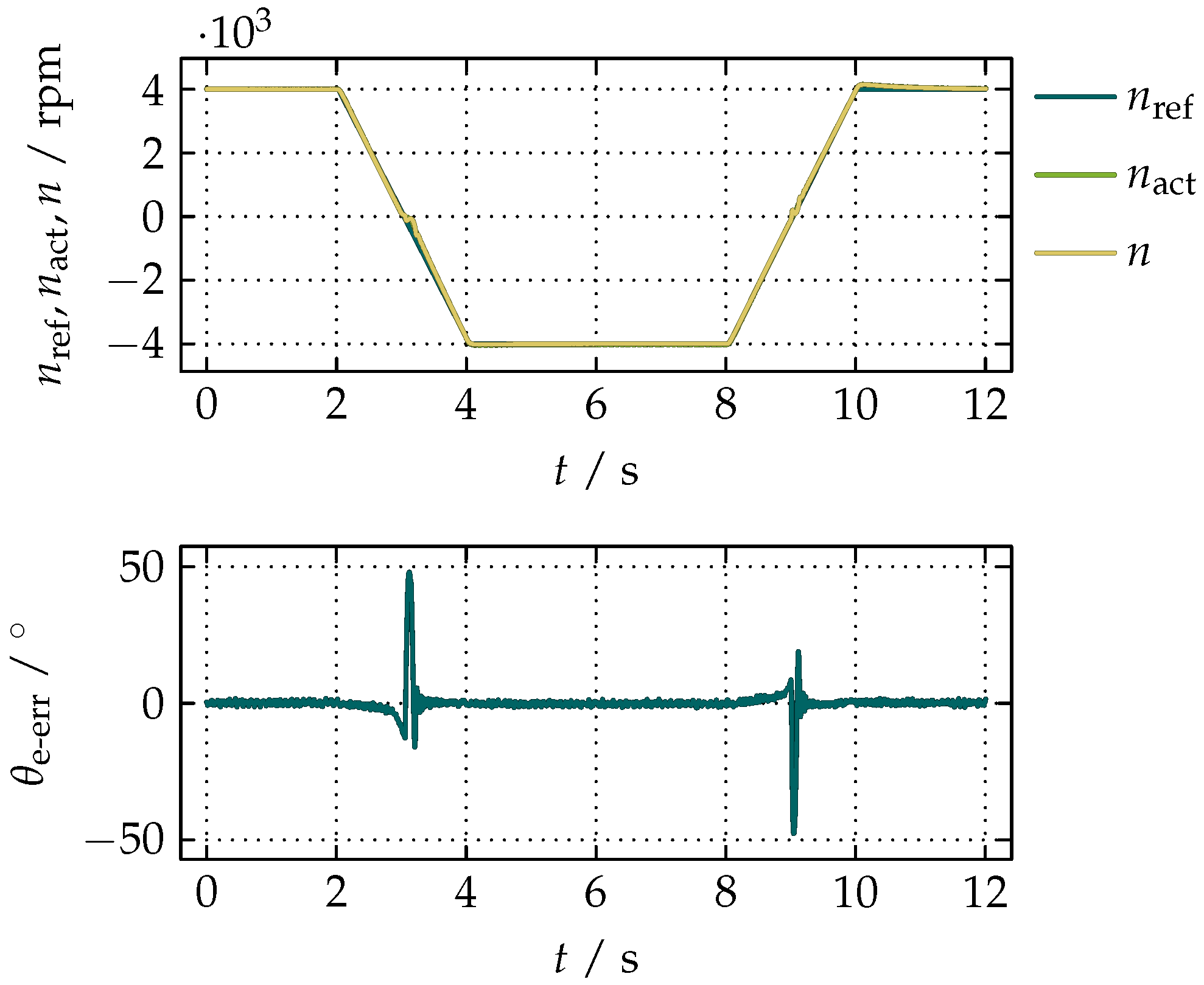
From Equation (60), it can be seen that $T_{\mathrm{em}}$ is proportional to $i_{\mathrm{sq}}$, which also explains the delayed startup. Since the load torque between 0 s and 35 s is 90% of $T_{\mathrm{n}}$, the initial current is not sufficiently high to create $T_{\mathrm{em}}$ that can overcome it. The current therefore rises until about 9 s when $T_{\mathrm{em}}$ overcomes the load torque and the rotor starts to spin. The sudden increase in n, and consequently in $n_{\mathrm{act}}$, is the result of the speed ramp that begins to rise at 1 s whose value at 9 s is approximately $600\mathrm{rpm}$. The plot of ${\theta }_{\mathrm{e}-\mathrm{err}}$ between 1 s and 9 s resembles the bottom plots in Figure 14, but looks like a random noise due to a limited number of samples that can be fetched by the used hardware. The observer is able to generate values of ${\theta }_{\mathrm{e}}$ and ${\omega }_{\mathrm{e}}$ due to the fact that all the necessary variables for the proposed compensation of the integrational drift are obtained from $v_{\mathrm{s}\alpha \mathrm{i}}$ and $v_{\mathrm{s}\beta \mathrm{i}}$, which are initially available. A smoother startup under a load can be achieved by setting a small reference of n and allowing the current to rise until $T_{\mathrm{em}}$ is sufficiently high to overcome the load torque. From the time period between 35 s and 60 s, when the motor is intermittently periodically loaded at $2000\mathrm{rpm}$, it can be seen that, despite the rapid changes in n, whose peak values are about $2000\pm 1500\mathrm{rpm}$, ${\theta }_{\mathrm{e}-\mathrm{err}}$ is within peak values +3.06° and −4.8° with the mean average value of +0.18°. A reversal of the unloaded motor from $4000\mathrm{rpm}$ to $-4000\mathrm{rpm}$ within 2 s and in the same time-span from $-4000\mathrm{rpm}$ back to $4000\mathrm{rpm}$ is presented in Figure 17.

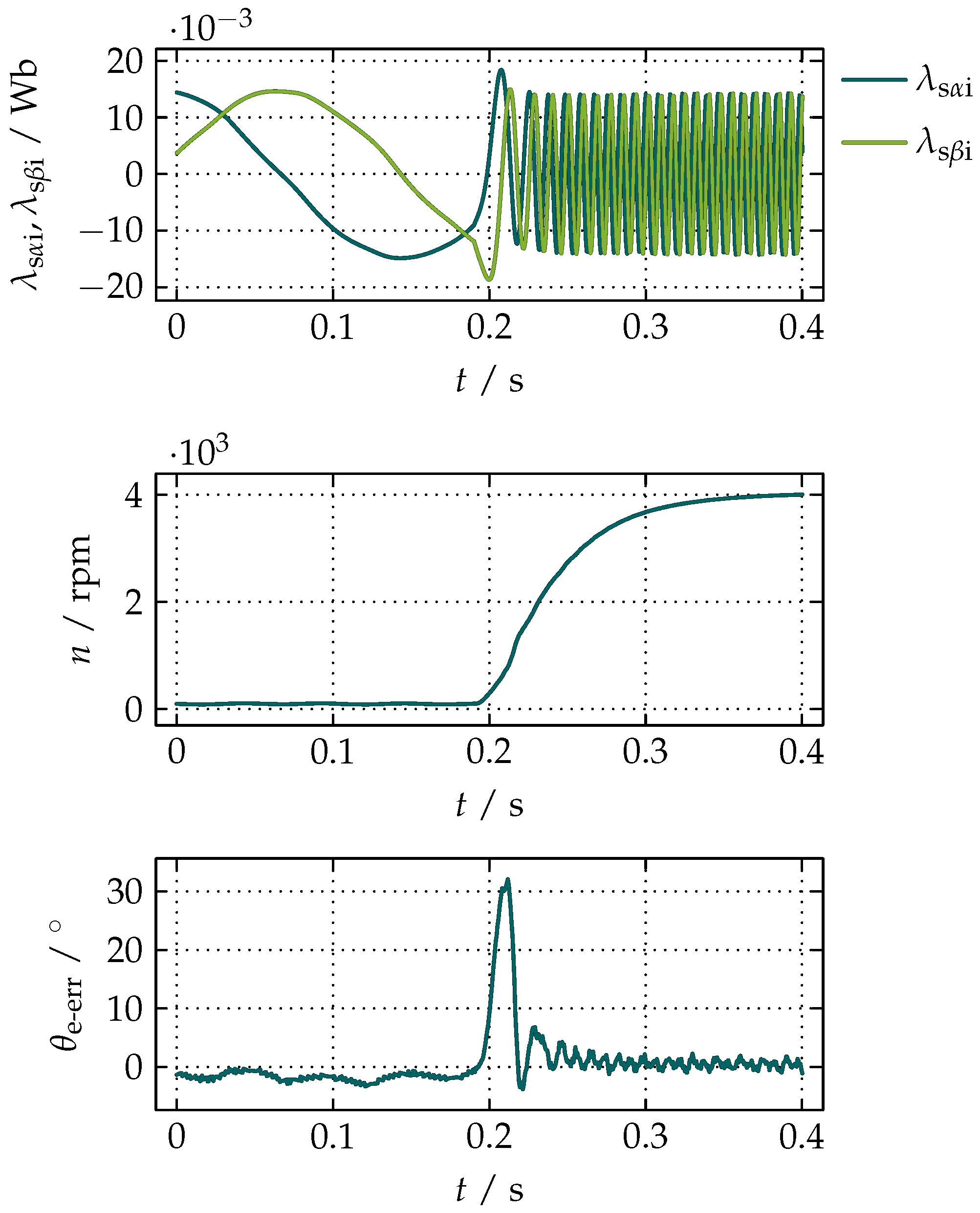
A small difference between $n_{\mathrm{act}}$ and n is noticeable only around zero when the distortion in the waveforms of the voltage and the current caused by a limited resolution of the measurement sensors and quantization errors increase the uncertainty of knowing the actual angular position of the rotor. The positive peak of ${\theta }_{\mathrm{e}-\mathrm{err}}$ is +47.95°, which within 0.31 s falls below 10% of its value, while the negative peak of −47.61° becomes smaller than 10% of its absolute value within 0.21 s. The dynamics of the proposed compensation is demonstrated in Figure 18 by applying the step in the speed from $100\mathrm{rpm}$ to $4000\mathrm{rpm}$ to the unloaded motor.

From the waveforms of ${\lambda }_{\mathrm{s}\alpha }$ and ${\lambda }_{\mathrm{s}\alpha }$ it is visible that the transient state is slightly longer than theoretically predicted due to limitations in the practical implementation of the pure differentiator used for obtaining ${\omega }_{\mathrm{e}}$ from ${\varphi }_v$, which, because of the white noise, requires a cascaded LPF whose cut-off frequency in the presented measurement was set to the electrical equivalent of the nominal value of n of the motor. Nonetheless, the resulting dynamics is exceptionally good, considering that the peak value of ${\theta }_{\mathrm{e}-\mathrm{err}}$ of 32.08° falls below 10% of its value within 24 ms.

It is important to mention that the measured values of $n_{\mathrm{act}}$ as well as ${\theta }_{\mathrm{e}-\mathrm{act}}$ were only used as reference values to demonstrate the performance of the proposed compensation of the integrational drift.

5. Discussion

The idea of compensating the integrational drift based on orthogonal properties of the input and output waveforms of the integrators in the stator reference frame has been demonstrated to be very effective. Although the presented measurements present a simple open-loop sensorless FOC for PMSMs, a clear distinction between the proposed compensation of the integrational drift presented in Figure 3 and the observer used for the demonstration of its effectiveness shown in Figure 1 needs to be made. Since a balanced three-phase power supply is required by the FOC to operate the motor effectively, the orthogonality of the input waveforms remains the only requirement for the proposed compensation of the integrational drift. The orthogonality is inherently ensured by the implementation in the stator reference frame, which makes the proposed compensation completely independent of the electrical parameters as well as the type of the motor, meaning that it can also be used for accurate estimations of magnetic flux in other types of machines. Another advantage of the proposed compensation lies in the fact that it does not need any optimization or tuning by the user. The fast response presented in Figure 18 comes from its design based on the basic arithmetic operations, which makes it faster than the methods presented in [18,19]. Unlike the methods referred in the Introduction, the proposed compensation does not effect the amplitude of the output waveforms, nor does it introduce any additional frequency-dependent phase shift in steady states, since it is built up of pure integrators. While the methods in [17,18,19] are able to start a motor from a standstill, the proposed compensation enables a startup with or without any load, although it is advisable to apply some sort of a startup strategy under a load for a smooth start. The simplicity of the proposed compensation enables it to be implemented on 16-bit DSPs, which makes it suitable for inexpensive applications.

References

- Vas, P. Sensorless Vector and Direct Torque Control; Oxford University Press: Oxford, UK, 1998; ISBN 9780198564652. [Google Scholar]
- Seyoum, D.; Grantham, C.; Rahman, M.F. Simplified Flux Estimation for Control Application in Induction Machines. In Proceedings of the 2003 IEEE International Electric Machines and Drives Conference (IEMDC’03), Madison, WI, USA, 1–4 June 2003; pp. 691–695. [Google Scholar]
- Čolović, I.; Kutija, M.; Sumina, D. Rotor Flux Estimation for Speed Sensorless Induction Generator Used in Wind Power Application. In Proceedings of the 2014 IEEE International Energy Conference (ENERGYCON), Cavtat, Croatia, 13–16 May 2014; pp. 23–27. [Google Scholar]
- Pellegrino, G.; Bojoi, R.I.; Guglielmi, P. Unified Direct-Flux Vector Control for AC Motor Drives. IEEE Trans. Ind. Appl. 2011, 47, 2093–2102. [Google Scholar] [CrossRef] [Green Version]
- Idris, N.R.N.; Yatim, A.H.M. An Improved Stator Flux Estimation in Steady-State Operation for Direct Torque Control of Induction Machines. IEEE Trans. Ind. Appl. 2002, 38, 110–116. [Google Scholar] [CrossRef] [Green Version]
- Shen, J.X.; Hao, H.; Wang, C.F.; Jin, M.J. Sensorless Control of IPMSM Using Rotor Flux Observer. COMPEL-Int. J. Comput. Math. Electr. Electron. Eng. 2012, 32, 166–181. [Google Scholar] [CrossRef]
- Xing, Z.; Wenlong, Q.; Haifeng, L. A New Integrator for Voltage Model Flux Estimation in a Digital DTC System. In Proceedings of the 2006 IEEE Region 10 Conference (TENCON 2006), Hong Kong, China, 14–17 November 2006. [Google Scholar]
- Xia, C.; Zhao, J.; Yan, Y.; Shi, T. A Novel Direct Torque Control of Matrix Converter-Fed PMSM Drives Using Duty Cycle Control for Torque Ripple Reduction. IEEE Trans. Ind. Electron. 2014, 61, 2700–2713. [Google Scholar] [CrossRef]
- Bose, B.K.; Patel, N.R. A Programmable Cascaded Low-Pass Filter-Based Flux Synthesis for a Stator Flux-Oriented Vector-Controlled Induction Motor Drive. IEEE Trans. Ind. Electron. 1997, 44, 140–143. [Google Scholar] [CrossRef]
- Norniella, J.G.; Cano, J.M.; Orcajo, G.A.; Rojas, C.H.; Pedrayes, J.F.; Cabanas, M.F.; Melero, M.G. Improving the Dynamics of Virtual-Flux-Based Control of Three-Phase Active Rectifiers. IEEE Trans. Ind. Electron. 2014, 61, 177–187. [Google Scholar] [CrossRef]
- Shin, M.H.; Hyun, D.S.; Cho, S.B.; Choe, S.Y. An Improved Stator Flux Estimation for Speed Sensorless Stator Flux Orientation Control of Induction Motors. IEEE Trans. Power Electron. 2000, 15, 312–318. [Google Scholar] [CrossRef]
- Zhang, Z.; Zhao, Y.; Qiao, W.; Qu, L. A Discrete-Time Direct-Torque and Flux Control for Direct-Drive PMSG Wind Turbines. In Proceedings of the 2013 IEEE Industry Applications Society Annual Meeting, Lake Buena Vista, FL, USA, 6–11 October 2013. [Google Scholar]
- Stojić, D.; Milinković, M.; Veinović, S.; Klasnić, I. Improved Stator Flux Estimator for Speed Sensorless Induction Motor Drives. IEEE Trans. Power Electron. 2014, 30, 2363–2371. [Google Scholar] [CrossRef]
- Hinkkanen, M.; Luomi, J. Modified Integrator for Voltage Model Flux Estimation of Induction Motors. IEEE Trans. Ind. Electron. 2003, 50, 818–820. [Google Scholar] [CrossRef]
- Hu, J.; Wu, B. New Integration Algorithms for Estimating Motor Flux over a Wide Speed Range. IEEE Trans. Power Electron. 1998, 13, 969–977. [Google Scholar] [CrossRef]
- Hurst, K.D.; Habetler, T.G.; Griva, G.; Profumo, F. Zero-Speed Tacholess IM Torque Control: Simply a Matter of Stator Voltage Integration. IEEE Trans. Ind. Appl. 1998, 34, 790–795. [Google Scholar] [CrossRef]
- Cho, K.R.; Seok, J.K. Pure-Integration-Based Flux Acquisition with Drift and Residual Error Compensation at a Low Stator Frequency. IEEE Trans. Ind. Appl. 2009, 45, 1276–1285. [Google Scholar] [CrossRef]
- Holtz, J. Sensorless Control of Induction Machines—With or Without Signal Injection? IEEE Trans. Ind. Electron. 2006, 53, 7–30. [Google Scholar] [CrossRef]
- Holtz, J.; Quan, J. Drift- and Parameter-Compensated Flux Estimator for Persistent Zero-Stator-Frequency Operation of Sensorless-Controlled Induction Motors. IEEE Trans. Ind. Appl. 2003, 39, 1052–1060. [Google Scholar] [CrossRef]
Figure 1.
A block diagram of the proposed observer for the flux-based sensorless FOC of PMSMs based on the voltage model in the stator reference frame.
Figure 2.
A block diagram of the sensorless FOC of PMSMs.
Figure 3.
A block diagram of the proposed compensation of the integrational drift in the time domain.
Figure 4.
An equivalent block diagram of the proposed compensation of the integrational drift in the Laplace domain.
Figure 5.
Bode plots common to both and showing the dependence of the frequency response of the proposed compensation on .
Figure 6.
Bode plots of and , with a common magnitude plot, showing the dependence of the frequency response of the proposed compensation on , where the superscripts of the phase plot index the transfer function for the positive direction of rotation, while the subscripts index the negative direction.
Figure 7.
A plot of with the component imposed by and imposed by in the time-domain for a step excitation on both inputs with .
Figure 8.
Figure 9.
The block diagram of the proposed compensation of the integrational drift used for simulations in MATLAB Simulink.