Mathematical Simulations and Analyses of Proportional Electro-Hydraulic Brakes and Anti-Lock Braking Systems in Motorcycles

Abstract

In the motorcycle industry, the safety of motorcycles operating at high speeds has received increasing attention. If a motorcycle is equipped with an anti-lock braking system (ABS), it can automatically adjust the size of the brake force to prevent the wheels from locking and achieve an optimal braking effect, ensuring operation stability. In an ABS, the brake force is controlled by an electro-hydraulic brake (EHB). The control valve inside the EHB was replaced with a proportional valve in this study, which differed from the general use of a solenoid valve. The purpose for this change was to precisely control the brake force and prevent hydraulic pressure oscillating in the piping. This study employed MATLAB/Simulink and block diagrams to establish a complete motorcycle ABS simulation model, including a proportional electro-hydraulic brake (PEHB), motorcycle motion, tire, and controller models. In an analysis of ABS simulation results, when traveling on different road surfaces, the PEHB could effectively reduce braking distance and solve the problem of hydraulic pressure oscillation during braking. The research demonstrated that this proportional pressure control valve can substitute the general solenoid valve in commercial braking systems. This can assist the ABS in achieving more precise slip control and improved motorcycle safety.

1. Introduction

The brake modules of modern motorcycles are generally equipped with an ABS to enable vehicles to stop within the shortest distance and motorcycle handles to be controlled to avoid obstacles and ensure driver safety. Brake performance is affected by the level of tire adhesion during the braking process. Tire adhesion refers to the acting force of the road surface on the tires and is also known as tire friction, which is divided into longitudinal and lateral directions. The sliding ratio between tires and the ground surface is defined as the slip [1,2,3,4,5,6].

$$S=\frac{V_v-V_w}{V_v}$$

(1)

where S is the brake slip, V_v is the vehicle speed, and V_w is the wheel speed.

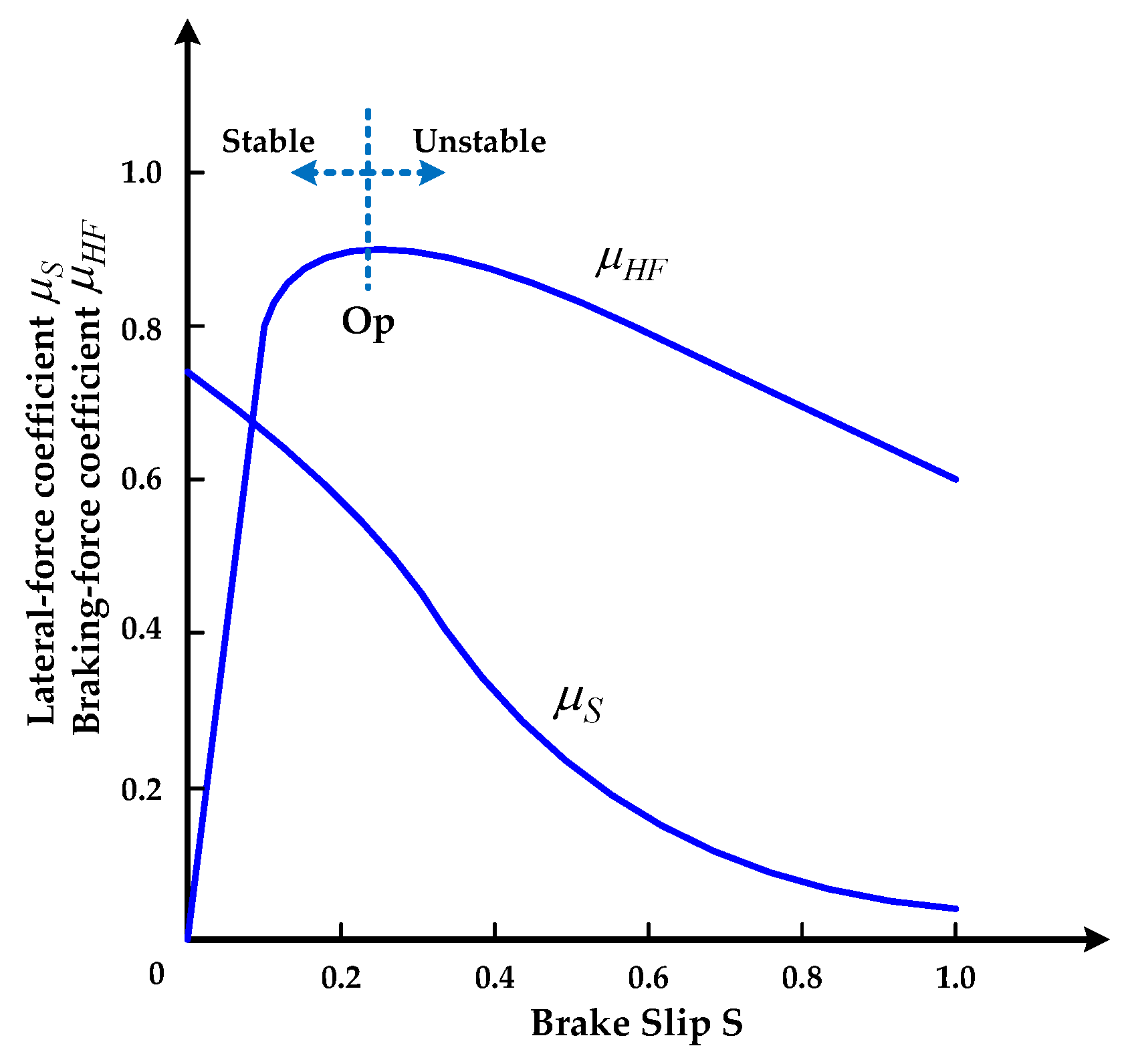
The curve in Figure 1 shows that optimal maneuverability was yielded when the slip was 0 (that is, when the vehicle speed was equal to the wheel speed) [7]. Conversely, the brake was locked if the slip was 1; thus, the wheel speed was 0 with no maneuverability. The highest point of longitudinal braking force Op served as the boundary for the stable and unstable zones, as well as the target for the optimal maneuverability.

When the rider presses the brake handle, the master cylinder generates brake pressure that is transmitted to the brake caliper of a wheel. At this time, the wheel speed sensor is responsible for constantly measuring wheel speed signals and providing these to the electronic control unit (ECU) of the ABS. After calculations by the microcomputer inside the ECU, control signals are sent to the EHB. The EHB is responsible for converting electrical control signals from the ECU into actual control actions of the solenoid valve to control brake pressure in the wheel cylinder. In the event of wheels locking, the brake pressure is controlled to a fixed level. If the wheel speed continues to decrease, the brake pressure will also decrease. When the ECU has determined that the wheels have resumed rotating, it will again increase the brake pressure to perform a braking action and repeat these actions until the vehicle has stopped [8,9,10]. The control circuit of an EHB actuator between master cylinder and wheel cylinder is shown in Figure 2 [11].

The general ABS control method drives the solenoid valve to increase, hold, and relief brake force. However, the solenoid valve is a discrete actuation component that can be controlled intermittently to adjust braking force in an approximate manner. The design of the proportional pressure control valve in this study combined the inlet and outlet valves into a three-port two-position solenoid valve, which was capable of accurately and rapidly yielding the optimal braking force through the continuous adjustment of the valve opening. Figure 3 shows a novel control circuit for a proportional electro-hydraulic brake (PEHB) actuator of a motorcycle [12]. Normal braking involves the rider pressing the brake handle to pressurize the master cylinder, and the pressure enters through the inlets of the reversing valve and proportional valve and is output from the caliper to drive the wheel cylinder to implement braking. The proportional valve is activated when the pressure is too high, and the inlet and outlet openings are adjusted according to the level of solenoid force to achieve an appropriate pressure drop in the caliper, thereby yielding the optimal slip control.

The brake performance of an ABS is determined through control logic, which is applied to overcome numerous uncertain parameters such as the time-varying characteristics of braking dynamics as well as environments, roads, and coefficients of friction. Various controlling strategies have been proposed and confirmed to control wheel slip effectively. The relevant mechanisms include optimal controller [10,13], fuzzy learning/logic controller [14,15,16], sliding mode controller [17], and proportional–integral–derivative (PID) control [18,19].

Of the relevant mechanisms, the PID controller is the most widely adopted across industries [20]. Various adjustment methods for PID have been proposed as described in [21]. Among them, the adjustment method for internal model control (IMC) was proposed by Rivera in 1986 [22]. The main operating principle of IMC is through feedback compensation. In addition to being able to compensate for disturbances and eliminate the uncertainty of the approximate model, the IMC can provide closed-loop stability and can also adjust to changes in the approximate model parameters. The model matching approach was employed in [23] to directly design the IMC according to the robust performance of the system. In the present study, a new type of brake actuator with a proportional solenoid valve was developed. Compared with the general solenoid valve with an on/off control, a proportional solenoid valve involves the advantage of continuous pressure servo control. To commercialize this invention, a basic PID controller was adopted, and a bang-bang controller was installed in front of the integrator so that the system can achieve precise and rapid ABS slip control.

2. Proportional Pressure Control Valve

The proportional pressure control valve consists of a proportional valve body and a proportional electromagnet.

2.1. Proportional Valve Body

The proportional valve body is composed of a proportional iron shell, a shuttle shaft with an iron core, and a valve body. Its design is shown in Figure 4 [24,25]. Outlet A and Inlet B are interconnected, and both are connected to the caliper. The openings of the spool and needle valves are adjusted through the shuttle shaft. The opening sizes of the two valve ports are proportional to each other. The needle valve port must be tightly closed when it is not actuated to avoid internal leakage. Therefore, the cone valve design was adopted, with the check valve in the shuttle shaft being used as a safety device. In the event that the shuttle shaft cannot be reset and the needle valve malfunctions, the caliper pressure can still be released through the check valve. The shuttle shaft force (F_m) equation is as follows:

$$F_m=F_{em}+F_{cal}$$

(2)

In addition, $F_m=P_m\cdot A_{sp}$, $F_{cal}=P_{cal}\cdot (A_{sp}-A_{ol})$

Substituting Equation (2)

$$P_{cal}=(F_m-F_{em})/(A_{sp}-A_{ol})$$

(3)

where F_em is the proportional solenoid force; F_cal is the caliper force; P_m is the master cylinder pressure; P_cal is the caliper pressure; A_sp is the spool valve cross-sectional area; and A_ol is the needle valve hole cross-sectional area.

2.2. Proportional Electromagnet

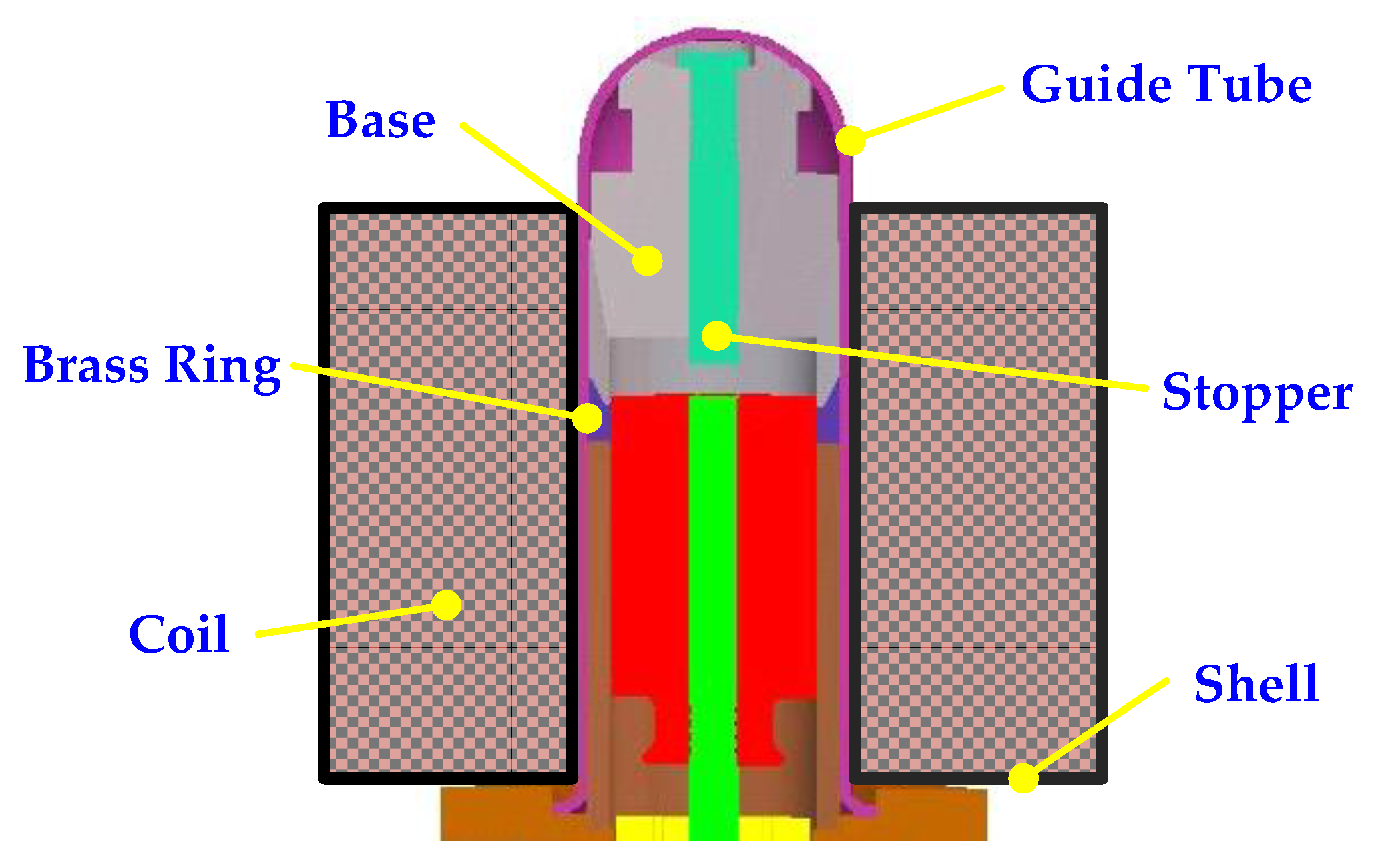
The actuation principle of the proportional electromagnet is the same as the general solenoid valve: the operating current passing through the coil causes the internal soft magnetic components to magnetize and generate a magnetic effect, thereby achieving the objective of mechanical movement due to electric excitation through energy conversion. Figure 5 shows the structure of the proportional electromagnet. The magnetic field direction and magnetic induction force are controlled by the current in the input coil, in turn causing the materials, such as base and iron core, to generate attraction due to excitation. The displacement of the valve shaft determines the flow volume and direction, whereas the spring provides the compressive force required for closing the valve port when no current is supplied. The main purpose of the brass ring is to change the direction of the magnetic field lines in order for them to enter the iron core through the guide tube, after which they are divided into two directions, entering the flange and axial center of the base through the radial and axial directions, respectively. The stopper is the component controlling the movement of the shuttle shaft in the linear region of operation.

Six types of simplified magnetic flux paths (Figure 6) were employed in this study as the design basis for the magnetic induction force, to deduce the direction for the magnetic field lines in the air gap between the metals, shown in

Table 1. The air gaps magnetic flux path model calculations.

Flux Path Model	Mean Path Length	$\mathbf{Permeance} ({\mathit{P}}_{\mathit{a}\mathit{i}\mathit{r}}$)
I	$\mathrm{g}$	$2\pi {\mu }_0(\mathrm{r}+\frac{\mathrm{g}}{2})\mathrm{h}/\mathrm{g}$
II	1.22$\mathrm{g}$	$3.3{\mu }_0(\mathrm{r}+\frac{\mathrm{g}}{2})$
III	1.22$\mathrm{g}$	$3.3{\mu }_0(\mathrm{r}+\frac{\mathrm{g}}{2})$
IV	$\sqrt{\mathrm{g}(\mathrm{g}+\mathrm{t})}$	$4{\mu }_0(\mathrm{r}+\sqrt{\mathrm{g}(\mathrm{g}+\mathrm{t})})\ln (\frac{\mathrm{g}+\mathrm{t}}{\mathrm{g}})$
V	$\sqrt{\mathrm{g}(\mathrm{g}+\mathrm{r})}$	$4{\mu }_0(\mathrm{r}+\mathrm{g}-\sqrt{\mathrm{g}(\mathrm{g}+\mathrm{r})})\ln (\frac{\mathrm{g}+\mathrm{r}}{\mathrm{g}})$
VI	$\mathrm{z}$	$\frac{{\mu }_0\pi }{z}{(\mathrm{r}+\mathrm{g}-2\mathrm{z}/\pi )}^2$

[26,27]. Here ${\mu }_0$ represents the permeability of air, $\mathrm{g}$ represents the air gap, $\mathrm{r}$ represents the iron core radius, $\mathrm{h}$ represents the right side distance between iron core and brass ring, $\mathrm{t}$ represents the thickness of brass ring, and $\mathrm{z}$ represents the distance from base to iron core.

Therefore, when a magnetic force is present and the magnetic flux is $\mathsf{\Phi }$, the magnetomotive force in the air gap ($F_{air}$) is as follows:

$$F_{air}=\mathsf{\Phi }{P}_{air}{}^{-1}$$

(4)

In soft magnetic materials, the magnetomotive force can be acquired by multiplying the magnetic field intensity ($H$) and the current path length ($l$). The magnetic field intensity can be determined according to its corresponding relationship with the magnetic flux density ($B$) through the B–H curve of each material. When a magnetic flux is present, the magnetomotive force of a soft magnetic material ($F_{steel}$) is as follows:

$$F_{steel}={\displaystyle {\sum }_{j=1}^i{H}_j}{l}_j$$

(5)

According Equations (4) and (5), magnetic flux and total magnetomotive force ($F_{sum}$) are generated when the number of coil turns ($N$) and the operating current ($I$) are input. In addition, Equation (6) shows that total magnetomotive force can be obtained from electrical energy through energy conversion. The relationship between the iron core displacement and the solenoid force ($F_{em}$) can be obtained through the principle of virtual work ($W$), as shown in Equations (7) and (8).

$$NI=F_{sum}=F_{air}+F_{steel}$$

(6)

$$W=\frac{1}{2}{\mathsf{\Phi }}^2{P}_{air}{}^{-1}$$

(7)

$$F_{em}=\frac{\partial W}{\partial \mathrm{z}}=\frac{{\mathsf{\Phi }}^2}{2}\cdot \frac{d}{d\mathrm{z}}(P_{{}^{air}}^{-1})=-\frac{{\mathsf{\Phi }}^2}{2}\cdot [P_{{}^{air}}^{-2}\frac{d}{d\mathrm{z}}{P}_{air}]$$

(8)

According to the above derivation, when the proportional electromagnet is completed, the magnetic flux can be calculated by inputting the operating current, thereby acquiring the magnetic flux density and magnetic field intensity of soft magnetic materials. The solenoid force can be obtained from the linear region of operation and used as a basis for the subsequent proportional valve control.

3. Mathematical Model and Controller

3.1. Mathematical Model of Motorcycle Motion

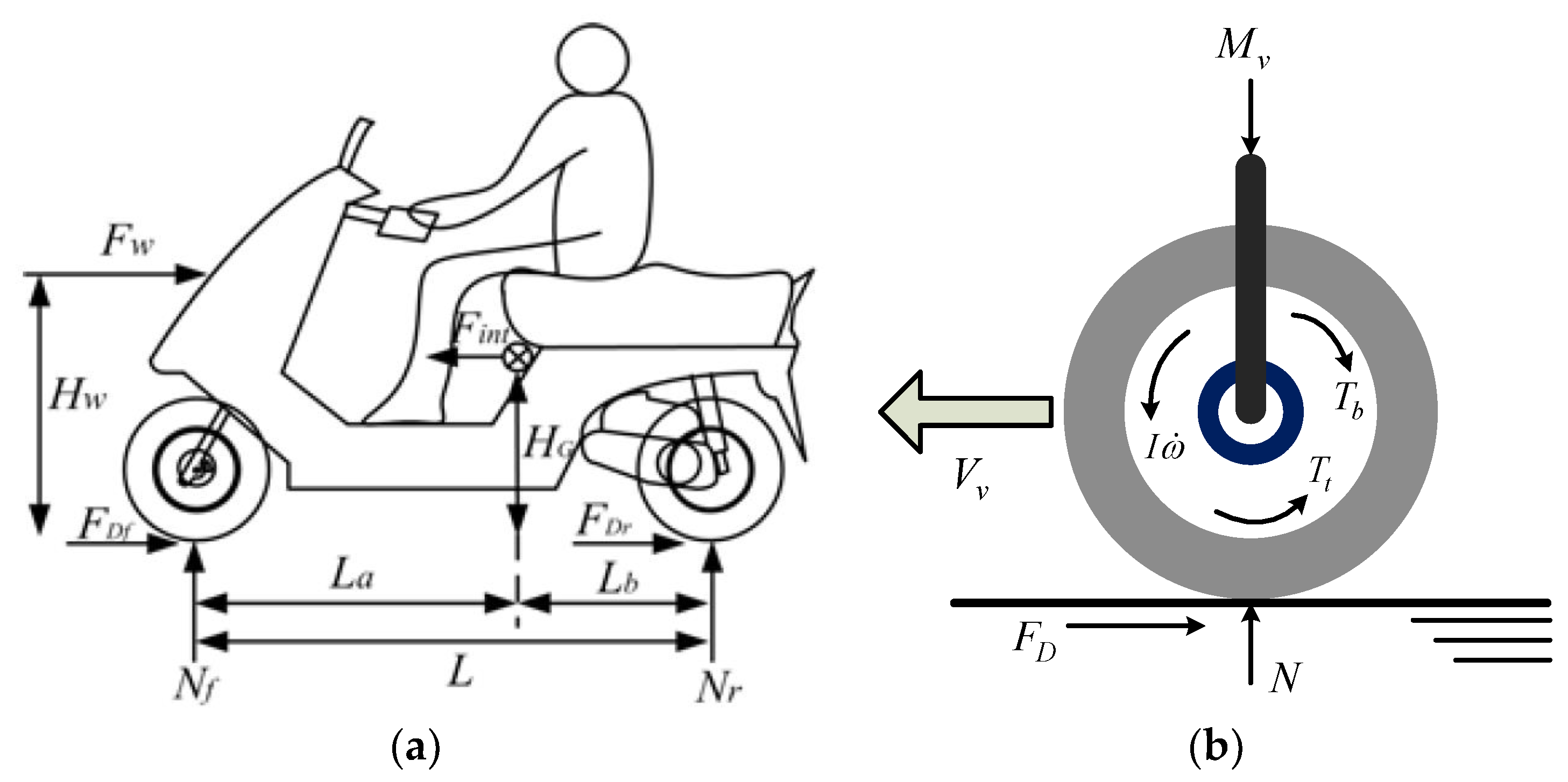
The motorcycle motion model provides calculations of vehicle dynamics that can be used to calculate relevant data during braking such as speed, slip, and braking distance. Figure 7a presents a simplified motorcycle motion model [28].

Its positive force $N$ acting on the wheel is expressed as follows:

$$\{\begin{array}{c}{N}_f=\left(1-e^{-t/t_f}\right)\left(M_v\cdot g\cdot L_b+F_{\mathrm{int}}\cdot H_G-F_w\cdot H_w\right)/L\\ N_r=\left(1-e^{-t/t_r}\right)\left(M_v\cdot g\cdot L_a-F_{\mathrm{int}}\cdot H_G+F_w\cdot H_w\right)/L\end{array}$$

(9)

In Equation (9), the subscript $f$ represents the action on the front wheel, whereas the subscript $r$ represents the action on the rear wheel. Among these actions, $M_v$ represents the total mass of the rider and the motorcycle, $L$ indicates the wheelbase between the front and rear wheels of the motorcycle, and $L_a$ and $L_b$, respectively, denote the distances between the front and rear wheels and the center of mass of the vehicle. $H_G$ represents the height of the center of the mass of the vehicle, $H_w$ indicates the average height of the wind force acting on the motorcycle, $t$ represents time, $t_f$ denotes the time-delay constant of the front shock absorber, and $t_r$ represents the time-delay constant of the rear shock absorber. $F_{\mathrm{int}}$ represents the inertial force of the vehicle and $F_w$ represents the longitudinal force of the wind. Their mathematical formulas are expressed as follows:

$$F_{\mathrm{int}}=M_v\cdot a$$

(10)

$$F_w=\frac{1}{2}\cdot {\rho }_w\cdot C_w\cdot A_w\cdot {\left(V_v+u_0\right)}^2$$

(11)

Among these, ${\rho }_w$ is air density, $C_w$ is the coefficient of air resistance, $A_w$ is the frontal area of the vehicle, $V_v$ is the vehicle speed, and $u_0$ is the wind speed. In this paper, the effect of wind speed is ignored, that is, it is assumed that $u_0=0$ and wind force is $F_w=0.155\cdot V_v^2$.

3.2. Wheel Braking Model

Figure 7b presents an analysis of the torque of a vehicle during braking, where $T_t$ represents the torque generated by the adhesive force of the road surface on the wheel and $T_b$ denotes the torque generated by the brake caliper on the wheel. These are expressed as follows:

$$T_t=F_D\cdot R_w$$

(12)

$$T_b=K_b\cdot P_{cal}$$

(13)

where $F_D$ represents the longitudinal adhesion value of the ground on the tire, $R_w$ is the tire radius, and $K_b$ is a torque constant and represents the constant of proportionality between the brake pressure and brake torque. The torque balance equation of the wheel is as follows:

$$I_w\cdot \dot{\omega }=T_t-T_b$$

(14)

where $I_w$ indicates the moment of inertia of the wheel and $\omega$ indicates its angular velocity. After obtaining the longitudinal force balance $\left(F_{\mathrm{int}}=F_w+F_D\right)$, the acceleration value of the vehicle can be expressed as follows:

$$a=\left(F_w+F_{Df}+F_{Dr}\right)/M_v$$

(15)

The integral of the aforementioned formula can be used to obtain the speed value of the vehicle, whereas integrating the formula twice can obtain braking distance. The motorcycle motion of symbols, parameters and values which are used in our simulation are described in

Table 2. The motorcycle motion data.

Symbol	Parameter	Value
$M_v$	total mass of the rider and the motorcycle	220 Kgf
$H_G$	height of the center of the mass of the vehicle	0.6 m
$H_w$	average height of the wind force acting on the motorcycle	0.7 m
$L$	wheelbase between the front and rear wheels of the motorcycle	1.2 m
$L_a$	distances between the front wheels and the center of mass of the vehicle	0.7 m
$t_f$	time-delay constant of the front shock absorber	0.2
$t_r$	time-delay constant of the rear shock absorber	0.1
${\rho }_w$	air density	1.18 kg/m3
$C_w$	coefficient of air resistance	0.48
$A_w$	frontal area of the vehicle	0.55 m2
$R_w$	tire radius	0.21 m

.

3.3. Tire and Ground Model

Several mathematical models can be applied to measure the acting forces of the ground and tires (hereafter referred to as tire force). This study employed the tire model presented by Dugoff to describe the relationship between longitudinal tire force $F_D$, slip $s$, and vehicle speed $V_v$. The equations for this Dugoff’s model are as follows [1,29]:

$$F_D=\{\begin{array}{cc}\frac{C_n\cdot s}{1-s}& when \frac{C_n\cdot s}{1-s}<\frac{\mu \cdot N}{2}\\ N\left[\mu -{\mu }^2\frac{N\left(1-s\right)}{4C_n\cdot s}\right]& when \frac{C_n\cdot s}{1-s}>\frac{\mu \cdot N}{2}\end{array}$$

(16)

where $C_n$ is the longitudinal stiffness of the tire, $\mu$ is the friction coefficient, and $N$ is the normal force of the tire.

The friction coefficient $\mu$ in the following equation, according to the experimental results of Dugoff’s, assumes that the friction coefficient and slip speed $V_v\cdot s$ change linearly under normal conditions, that is,

$$\mu ={\mu }_{no}\left(1-A_n\cdot V_v\cdot s\right)$$

(17)

where ${\mu }_{no}$ is the friction coefficient during no slip, and $A_n$ is the adhesion reduction coefficient.

On wet road surfaces, the friction coefficient decreases exponentially with an increase in slip speed, that is,

$$\mu ={\mu }_{no}\cdot \exp \left[-\frac{V_v\cdot s}{V_c}\right]$$

(18)

where $V_c$ is the characteristic speed and is a constant; its size is related to the root mean square texture height.

3.4. PEHB Mathematic Model Analysis

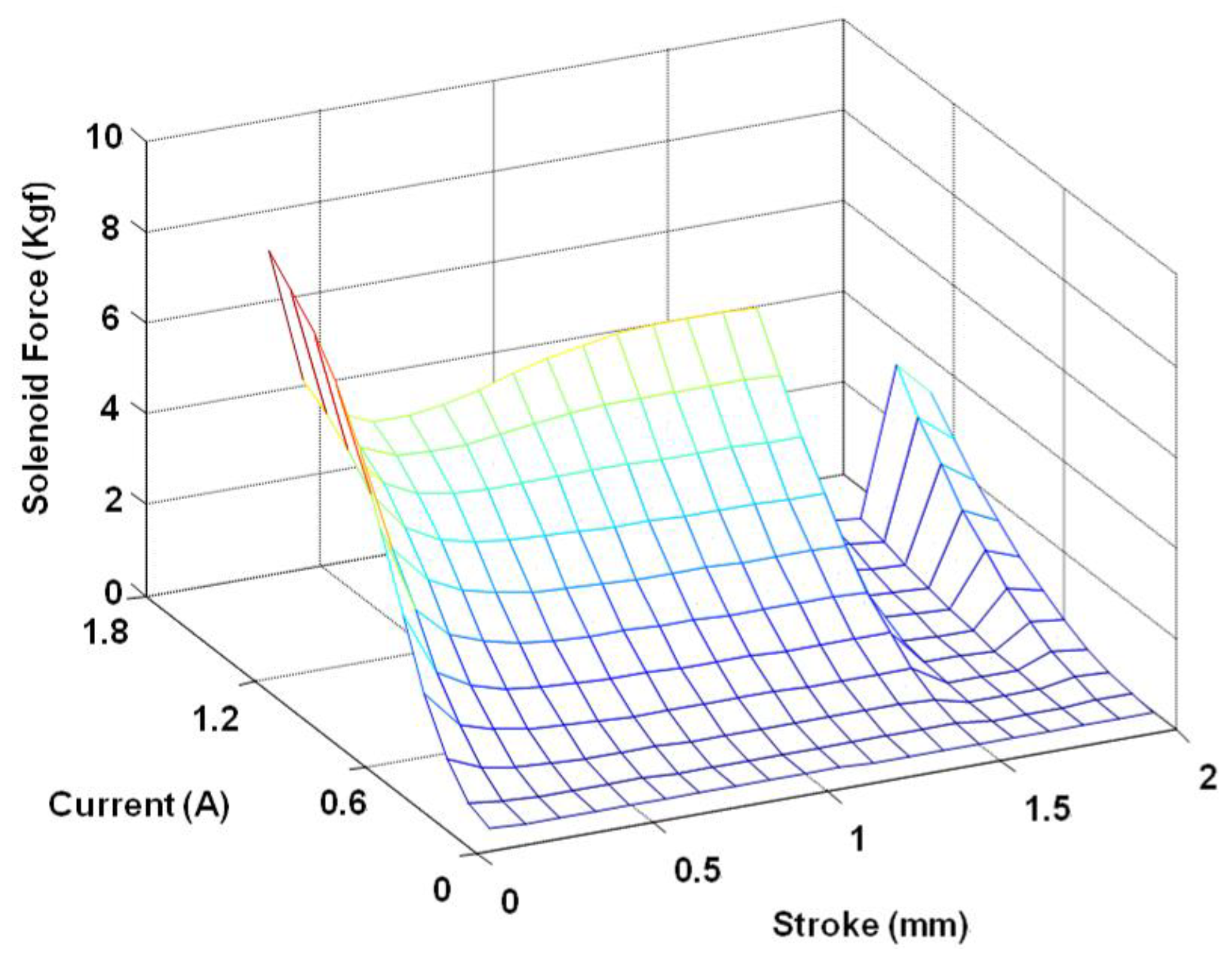
The PEHB design configuration (Figure 3) is primarily composed of a proportional control valve, motor pump, accumulator, caliper set, and hydraulic pipes. First, this study established a relationship database of proportional solenoid force, current, and stroke (Figure 8). The system can obtain solenoid force data through the look-up table after input current and stroke.

When the direction of the solenoid force of the proportional solenoid is defined as positive, the equation of motion on the shuttle shaft is as follows:

$$F_{em}=F_m+M_s\cdot \ddot{X}+B\cdot \dot{X}+K(X_c+X)$$

(19)

where $M_s$ is the shuttle shaft and iron core mass; $B$ is the damping coefficient; $K$ is the spring constant; $X_c$ is the spring initial compression value; and $X$ is the shuttle shaft stroke.

The valve body is a variation of a three-port proportional solenoid valve. Its mathematic model comprises two functions, namely those of the inlet valve and outlet valve. The inlet valve is a spool valve. The flow rate–pressure equation that describes the brake fluid flowing through the orifice is

$$Q=C_d\cdot \frac{\pi \cdot d}{4}\left(d-X\right)\cdot \sqrt{\frac{2}{\rho }\left(P_1-P_2\right)}$$

(20)

where $Q$ is the flow rate; $d$ is the spool valve hole diameter; $\rho$ is the fluid mass density; $C_d$ is the discharge coefficient; and $P_1$ and $P_2$ represent the pressure before and after the fluid flows through the orifice, respectively. The brake fluid may flow from either end to the other depending on which side exhibits the higher pressure.

The outlet valve parameters are identical to those of the inlet valve. The only difference between the inlet valve and the outlet valve is that the outlet valve is a needle valve that normally remains closed. After excitation, the degree to which the outlet valve opens is adjusted by the shuttle shaft interlocked with the iron core. The framework of the interior component blocks of the outlet valve is identical to that of the inlet valve. The coning angle of the needle valve is $\theta$. Accordingly, the area of the port is as follows:

$$A_0=\pi \cdot d\cdot X\cdot \sin (\theta /2)$$

(21)

The major component of the caliper is a piston. The brake fluid from the EHB pushes the piston, causing the caliper to clench the brake disc and stop the car. The spring serves to restore the caliper to its original position. Therefore, the equation of the caliper is as follows:

$$F_{cal}=K_c\cdot X_P$$

(22)

Because $F_{cal}=P_{cal}\cdot A_c$ and $X_p=V_c/A_c$, the previous equation can be rewritten as follows:

$$d{P}_{cal}=\frac{d{V}_c\cdot K_c}{A_c^2}$$

(23)

where $K_c$ is the coefficient of caliper spring; $X_P$ is the stroke of caliper piston; $V_c$ is the volume of caliper piston; and $A_c$ is the caliper piston cross-sectional area.

The strokes of the caliper involve two stages. In the first stage, the caliper does not make contact with the brake disc. In the second stage, the caliper is regarded as a rigid hydraulic chamber, described through the following equation:

$$d{P}_{cal}=\beta \cdot \frac{d{V}_c}{V_c}$$

(24)

where $\beta$ is the bulk modulus of the liquid.

Once the ABS decompression cycle begins, the two ports adjust their degrees of opening. The brake fluid flows through the outlet valve and out the caliper, entering the oil return pipe. Subsequently, the brake fluid is stored in the pressure accumulator. The return pump is activated to draw the fluid back into the brake pipe to avoid a pressure increase in the oil return area, which may result in brake-release failure.

The structure of the pressure accumulator is similar to that of the caliper in that the pressure accumulator is also composed of a piston and a restoring spring; however, its spring constant and cross-sectional area are smaller.

A reciprocating fixed-displacement pump is positioned between the pressure accumulator and the oil return pipe. The return pump is activated by the DC motor. In the mathematic model, a fixed-frequency square wave represents the motor. In the mathematical equation representing the return pump function, the difference between the inlet pressure and the atmospheric pressure is derived and then multiplied by the displacement gain, and the maximum discharge is then added.

The PEHB model of symbols, parameters and values which are used in our simulation are described in

Table 3. The PEHB model data.

Symbol	Parameter	Value
$M_s$	shuttle shaft and iron core mass	0.1 Kgf
$B$	damping coefficient	0.20 Kgf-s/mm
$K$	spring constant	0.18 Kgf/mm
$X_c$	spring initial compression value	0.3 mm
$d$	spool valve hole diameter	1.2 mm
$\theta$	coning angle of the needle valve	25
$\beta$	bulk modulus of the liquid	190 Kgf/mm2
$P_{cal}/V_c$	Caliper pressure per unit volume	0.06 Kgf/mm5

.

3.5. Traditional Discrete Switch Control

The switch control of a traditional solenoid valve, which must be open or closed, can be represented by Figure 9. This type of discrete switch control has a control signal of 1 when the index is greater than 0. Applied to this paper, this represented full supercharge; the solenoid valve remained open during the entire sampling time. Conversely, if the index is less than 0, the control signal is −1, signifying full depressurization; it remains in a depressurized state during the entire sampling time. In such a situation, the control signal is not fine enough to achieve the desired control effect. To improve this performance, the sampling period can be shortened (i.e., increase the sampling frequency) to achieve immediate control.

3.6. Proportional–Integral–Derivative Controller

The proportional–integral–derivative (PID) controller, which has a long history of use, is a feedback control method commonly found in industrial control and is widely used in various fields. The PID has become a common and reliable technical tool in industrial control because of its simple structure, favorable stability, and ease of operation and adjustment. It is composed of a proportional unit, integral unit, and derivative unit. By adjusting the parameters of controller $K_p$, $K_i$, and $K_d$, the control system can be adjusted to satisfy design requirements. The responding result can be expressed in terms of how rapidly the controller responds to an error, the degree to which the controller overshoots, and the degree of system oscillation. The input to the PID controller is the error value or the signal derived from this value. The output (controlled variable) is the result of the sum of three algorithms. Defining $u\left(t\right)$ as the control output, the PID algorithm can be expressed as Equation (25); its block diagram is presented in Figure 10.

$$u\left(t\right)=K_{p}e\left(t\right)+K_i{\displaystyle {\int }_0^{t}e\left(\tau \right)} d\tau +K_d\frac{d}{dt}e\left(t\right)$$

(25)

The transfer function of PID controller can be described as:

$$\begin{array}{cc}\hfill G_c\left(s\right)& =\frac{U\left(s\right)}{E\left(s\right)}=K_p+\frac{K_i}{s}+K_{d}s\hfill \\ & =K_p\left(1+\frac{1}{T_{i}s}+T_{d}s\right) Where T_i=\frac{K_p}{K_i} , T_d=\frac{K_d}{K_p}\hfill \end{array}$$

(26)

where $T_i$ is the integral time constant and $T_d$ is the derivative time constant.

4. Simulation and Results Analysis

For this analysis, MATLAB/Simulink was used to construct a PEHB system. The simulation commands were primarily step and triangular wave commands. Step commands confirmed the response time and triangular wave commands confirmed the following status and linearity, and this depressurization result was analyzed to determine whether it could satisfy ABS control requirements. Subsequently, a complete motorcycle ABS simulation model was established, which comprised a motorcycle motion model, tire model, and a controller model. A comparison of EHB and PEHB models was also conducted. The EHB model used a bang-bang controller for slip feedback control, whereas the PEHB model employed a PID controller for slip feedback control. Figure 11 shows a block diagram of the anti-lock braking control system. Additionally, different road surface condition control results and braking distance comparisons were analyzed.

4.1. PEHB System Simulations and Analyses

In this study, a mathematical model was first constructed and analyzed for a single-wheel PEHB, as presented in Figure 12 and Figure 13. MATLAB/Simulink was used to connect each block excluding the coil and iron core, which were voltage signals; the primary parameters considered were air gaps, hydraulic pressure, and flow. To simulate a braking situation, the inlet valve produced a constant pressure of 100 bars. After the coil received the excitation command, the iron core began to move and the inlet and outlet valves were adjusted to a certain opening degree. When the hydraulic pressure used for the shaft was balanced with the solenoid force, the opening degree was maintained, and the brake caliper decreased the caliper pressure moderately; that is, skidding due to locking from the application of excessive braking force could be prevented, and the fluid flowing from the outlet valve was carried away by the motor pump.

Figure 14 shows step wave command relief simulation results. It shows that when the voltage is lower than 1 V, the solenoid force is short to open the valve port. The corresponding caliper pressure drops and iron core stroke for 2, 3, 4, 5, 6, 7, 8, 9, and 10 V are, respectively, 5.5, 19.8, 36.6, 55.4, 76.9, 98.0, 99.3, 99.4 and 99.5 bars and 0.17, 0.29, 0.38, 0.45, 0.55, 0.73, 0.78, 0.79 and 0.8 mm. The simulation results show that the caliper pressure and iron core stroke are saturated when the command is greater than 8 V. The proportional valve simulation remains stable after pressure relief and meets with application requirements, and it can be used as a reference for the internal controller of the subsequent ABS module as the basis for the slip control calculation.

Figure 15 shows the triangular wave command relief simulation results. The proportional electromagnet is not actuated at command 2.5 V or less, and the pressure drop is 100 bars above 8 V. The pressure drop between 2.5 V and 8 V is linear, and the relationship between voltage and pressure drop can be derived as 18.2 bars/V. The caliper pressure follows the command well and linearly, and the pressure does not have vibration when the valve is fully open.

4.2. Motorcycle ABS Simulation Model with an EHB

Figure 16 depicts the brake mathematical model of the bang-bang controller using MATLAB/Simulink, which represents the action characteristic (i.e., it must be open or closed) of the solenoid valve. After the hydraulic pressure transfer function was applied and the hydraulic lag time constant TB is 0.5 s, it was integrated to obtain pressure change. Finally, it was applied to the brake caliper and the brake force was adjusted. Figure 17 depicts the establishment of a complete motorcycle ABS simulation model, which comprised an EHB model, motorcycle motion model, tire model, and integrated bang-bang controller model.

The slip command was fixed at 0.2 and the initial vehicle speed and front and rear wheel speeds were controlled at 60 km/h. The brake force changed the wheel and vehicle speeds. The speed difference between the two was converted into slip, that is, the feedback factor of the ABS control loop. The simulation results are presented in Figure 18; the entire process was approximately 2.4 s, braking distance was approximately 22 m, and during the process the wheel speed clearly oscillated because of the on-off control. After 0.5 s, the slip oscillated at approximately 0.2 ± 0.1 and the front wheel exhibited greater inertial force due to braking and therefore had a higher frequency. After 2 s, the vehicle speed was decreased to less than 10 km/h; the slip increased due to loop gain and was unstable and divergent. This was an inherent phenomenon of the ABS; thus, in general ABS controls, the ABS function must be turned off when the vehicle speed is less than approximately 10 km/h. First-order damping was applied to the bang-bang controller to alleviate the pressure output changing into a ramp change. Generally, the braking process is affected by inertia, resulting in an increase in the normal force of the front wheel and a decrease in the rear wheel. By controlling the brake component measurements the same way, the simulations demonstrated that the front wheel would skid earlier, and the slip would continue to oscillate and be unable to stabilize. In other words, under normal ABS control, the average discharge pressure of the front wheel is higher than that of the rear wheel. The average pressure of the simulation results was approximately 50 bars for the rear wheel, which was greater than that of the front wheel (40 bars).

4.3. Motorcycle ABS Simulation Model for New PEHB

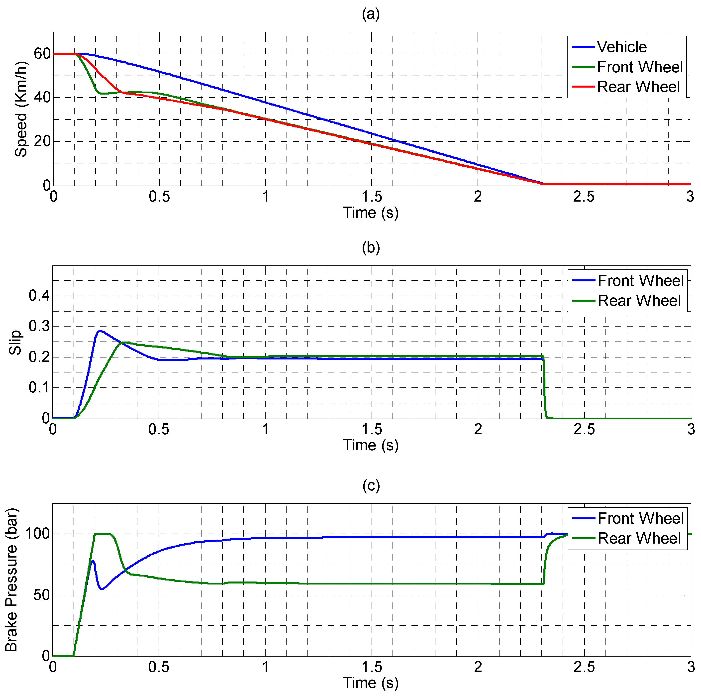
The solenoid valve brake actuator in Figure 19 was replaced with the mathematical models of the PEHB and PID controller for ABS control simulations. The block diagram of the controller is provided in Figure 20. In the PID controller, to increase integral compensation, a conditional function similar to that of the bang-bang system was added in front of the integrator. Thus, for the integrator, this was equivalent to receiving a gain of a previous order that is changeable. Figure 21 illustrates the differences in simulation results for the system with and without the bang-bang controller in front of the integrator in the PID controller. After the bang-bang controller was installed, front–rear wheel slip control with a target value of 0.2 was conducted; the results indicated that during the initial stage of the brake, the overshoot of the slip control was small. Subsequently, the steady-state error was eliminated to achieve the target value, thereby reducing the braking distance. Finally, after the controller parameters were adjusted by Ziegler and Nichols method, the controller parameters can achieved K_p = −40, K_i = −5, and K_d = −0.5.

As presented in Figure 22a, under initial conditions of a dry road surface and identical vehicle speed and front and rear wheel speeds, the braking sequence started at 0.1 s, at which time slip control was also initiated. The vehicle speed and front and rear wheel speeds decreased steadily to a halt, and the braking distance was further reduced to 21 m.

The slip trends of the front and rear wheels are provided in Figure 22b. The slip was controlled within a stable region, and the slip of the front and rear wheels were precisely controlled at a target value of 0.2 at 0.5 s and 0.8 s, respectively. The pressures of the front and rear wheel calipers are depicted in Figure 22c; the stable pressure indicates that the front wheel is higher. At the beginning, because the slip of the front wheel had exceeded the target value at 0.2 s, the brake force had to be removed as a response. After entering a precise slip control loop, it was revealed that brake pressure of the front wheel was greater than that of the rear wheel, which was consistent with the normal braking model of a motorcycle.

As depicted in Figure 23a, under the initial conditions of a wet road surface and identical vehicle speed and front and rear wheel speeds, the braking sequence started at 0.1 s, at which time the slip control was initiated. The vehicle speed and front and rear wheel speeds decreased steadily to a halt; however, the braking time increased by 0.7 s compared with that obtained for dry road surface conditions.

The slip trends of the front and rear wheels are presented in Figure 23b. Skidding was more evident in the front wheel, and was at its maximum at approximately 0.32. However, the slips of the front and rear wheels were both precisely controlled at a target value of 0.2 at 0.78 s. The pressures of the front and rear wheel calipers are depicted in Figure 23c. Because the slip of the front wheel exceeded the target value at 0.2 s, the brake force had to be removed as a response; at the same time, a precise slip control loop was applied. However, because the road surface was wet and the friction coefficient was smaller, to avoid skidding, the brake force applied should not be overly strong. Because the steady-state pressure was less than that of the dry road surface (approximately 60 bars), the braking distance was longer than that of the dry road surface.

4.4. Analyses of Simulation Results

Figure 24 presents a comparison of the braking distances for four braking models, including the braking distances of a traditional EHB and the PEHB of this study on dry and wet road surfaces, as well as the braking distance without the addition of the ABS. The simulation results revealed that the PEHB could effectively reduce braking distance, and that vehicles without an ABS had the longest braking distances due to vehicle brake locking, which resulted in skidding. A summary of the parameters of each simulation is shown in

Table 4. A summary of the parameters of each simulation.

Control Module and Mode	Road State	Braking Time (s)	Stopping Distance (m)	Slip (Steady State)
PEHB + PID	Dry	2.29	20.88	0.2 ± 0.06
PEHB + PID	Wet	2.97	26.42	0.2 ± 0.03
EHB + Bang-Bang	Dry	2.40	21.73	0.2 ± 0.1
Without ABS	Dry	>3	>34.35	1

.

5. Conclusions

This study primarily integrated the inlet and outlet valves of a market EHB into a set of proportional pressure control valves to achieve precise brake force control. MATLAB/Simulink was used to establish the mathematical model of the PEHB actuator. The simulation results demonstrated that this actuator had achieved a stable adjustment of depressurization control as well as favorable linear precision and repeatability; therefore, it can be applied to the ABS for slip control. Additionally, a complete motorcycle ABS simulation model was established, and simulations and analyses were performed for the wheel speed, slip, and brake force of the EHB and PEHB on different road surfaces during braking. Through the simulation results, it was demonstrated that the PEHB could achieve more favorable stability and speed during breaking, in addition to precisely achieving the target values during slip control and effectively reducing braking distance.

References

- Wu, M.C.; Shih, M.C. Simulated and experimental study of hydraulic anti-lock braking system using sliding-mode PWM control. Mechatronics 2003, 13, 331–351. [Google Scholar] [CrossRef]
- Qiuetal, Y.; Liang, X.; Dai, Z. Backstepping dynamic surface control for an anti-skid braking system. Control Eng. Pract. 2015, 42, 140–152. [Google Scholar]
- Tanelli, M.; Sartori, R.; Savaresi, S.M. Combining Slip and Deceleration Control for Brake-by-wire Control Systems: A Sliding-mode Approach. Eur. J. Control 2007, 6, 593–611. [Google Scholar] [CrossRef]
- Lv, C.; Zhang, J.; Li, Y.; Yuan, Y. Novel control algorithm of braking energy regeneration system for an electric vehicle during safety–critical driving maneuvers. Energy Convers. Manag. 2015, 106, 520–529. [Google Scholar] [CrossRef]
- Patra, N.; Datta, K. Observer based road-tire friction estimation for slip control of braking system. Procedia Eng. 2012, 38, 1566–1574. [Google Scholar] [CrossRef]
- Bhandari, R.; Patil, S.; Singh, R.K. Surface prediction and control algorithms for anti-lock brake system. Transp. Res. Part C 2012, 21, 181–195. [Google Scholar] [CrossRef]
- Choa, J.R.; Choia, J.H.; Yoo, W.S.; Kim, G.J.; Woo, J.S. Estimation of dry road braking distance considering frictional energy of patterned tires. Finite Elem. Anal. Des. 2006, 42, 1248–1257. [Google Scholar] [CrossRef]
- Ivanov, V.; Savitski, D.; Augsburg, K.; Barber, P.; Knauder, B.; Zehetner, J. Wheel slip control for all-wheel drive electric vehicle with compensation of road disturbances. J. Terramech. 2015, 61, 1–10. [Google Scholar] [CrossRef]
- Aksjonov, A.; Augsburg, K.; Vodovozov, V. Design and Simulation of the Robust ABS and ESP Fuzzy Logic Controller on the Complex Braking Maneuvers. Appl. Sci. 2016, 6, 382. [Google Scholar] [CrossRef]
- Mirzaei, M.; Mirzaeinejad, H. Optimal design of a non-linear controller for anti-lock braking system. Transp. Res. Part C 2012, 24, 19–35. [Google Scholar] [CrossRef]
- Wang, B.; Huang, X.; Wang, J.; Guo, X.; Zhu, X. A robust wheel slip ratio control design combining hydraulic and regenerative braking systems for in-wheel-motors-driven electric Vehicles. J. Frankl. Inst. 2015, 352, 577–602. [Google Scholar] [CrossRef]
- Chen, C.P.; Chiang, M.H. Development of Proportional Pressure Control Valve for Hydraulic Braking Actuator of Automobile ABS. Appl. Sci. 2018, 8, 639. [Google Scholar] [CrossRef]
- Drakunov, S.; Özgüner, Ü.; Dix, P.; Ashrafi, B. ABS control using optimum search via sliding modes. IEEE Trans. Control Syst. Technol. 1995, 3, 79–85. [Google Scholar] [CrossRef]
- Keshmiri, R.; Shahri, A.M. Intelligent ABS Fuzzy Controller for Diverse Road Surfaces. Int. J. Mech. Syst. Sci. Eng. 2007, 1, 257–262. [Google Scholar]
- Precup, R.-E.; Preitl, S.; Faur, G. PI predictive fuzzy controllers for electrical drive speed control: Methods and software for stable development. Comput. Ind. 2003, 52, 253–270. [Google Scholar] [CrossRef]
- Chaoui, H.; Sicard, P. Adaptive fuzzy logic control of permanent magnet synchronous machines with nonlinear friction. IEEE Trans. Ind. Electron. 2012, 59, 1123–1133. [Google Scholar] [CrossRef]
- Choi, S.B.; Bang, J.H.; Cho, M.S.; Lee, Y.S. Sliding mode control for anti-lock brake system of passenger vehicles featuring electrorheological valves. Proc. Inst. Mech. Eng. Part D J. Automob. Eng. 2000, 216, 897–908. [Google Scholar] [CrossRef]
- Jiang, F.; Gao, Z. An application of nonlinear PID control to a class of truck ABS problems. In Proceedings of the 40th IEEE Conference on Decision and Control, Orlando, FL, USA, 4–7 December 2001; pp. 516–521. [Google Scholar]
- Aparow, V.R.; Ahmad, F.; Hudha, K.; Jamaluddin, H. Modelling and PID control of antilock braking system with wheel slip reduction to improve braking performance. Int. J. Veh. Saf. 2013, 6, 265–296. [Google Scholar] [CrossRef]
- Astrom, K.; Hagglund, T. PID Controller: Theory, Design and Tuning; Instrument Society of America: Research Triangle Park, NC, USA, 1995. [Google Scholar]
- Astrom, K.; Hagglund, T. Advanced PID Design; ISA-The Instrumentation Systems, and Automation Society: Research Triangle Park, NC, USA, 2005. [Google Scholar]
- Rivera, D.E.; Morari, M.; Skogestad, S. Internal model control. 4. PID controller design. Ind. Eng. Chem. Process Des. Dev. 1986, 25, 252–265. [Google Scholar] [CrossRef]
- Jin, Q.B.; Liu, Q. IMC-PID design based on model matching approach and closed-loop shaping. ISA Trans. 2014, 53, 462–473. [Google Scholar] [CrossRef] [PubMed]
- Chen, C.P.; Tung, C.; Chen, C.A. A Proportional Electro-Hydraulic Braking Control Valve. Taiwan, 2010. Patent No. I320374, 11 February 2010. [Google Scholar]
- Chen, C.A.; Tung, C.; Chen, C.P. The Proportional Solenoid Module for a Hydraulic System. Patent No. I474350, 21 February 2015. [Google Scholar]
- Lee, C.O.; Song, C.S. Analysis of the solenoid of a hydraulic proportional compound valve. In Proceedings of the 35th National Conference on Fluid, Chicago, IL, USA, 13–15 November 1979; pp. 21–30. [Google Scholar]
- Chen, Y.N.; Kuo, W.H. Analysis and Design of Proportional Pressure Control Valve. Master’s Thesis, National Taiwan University, Taipei, Taiwan, 1987. [Google Scholar]
- Lu, C.Y.; Shih, M.C. Design and Control of the Hydraulic Anti-Lock Brake System for a Light Motorcycle. Ph.D. Thesis, National Cheng Kung University, Tainan, Taiwan, 2005. [Google Scholar]
- Dugoff, H.; Fancher, P.S.; Segel, L. An Analysis of Tire Traction Properties and Their Influence on Vehicle Dynamic Performance; SAE Paper No. 700377; SAE International: Warrendale, PA, USA, 1970. [Google Scholar]
Figure 1.
Relationship between tire adhesion coefficient and brake slip curve.
Figure 2.
The control circuit of an EHB actuator: (a) structure; and (b) ABS control mode.
Figure 3.
The novel control circuit for a proportional electro-hydraulic brake (PEHB) actuator of a motorcycle.
Figure 4.
The structure of the proportional valve body for a PEHB.
Figure 5.
The structure of the proportional electromagnet for a PEHB.
Figure 6.
Six types of simplified magnetic flux paths.
Figure 7.
A simplified motorcycle structure: (a) motion model; and (b) single wheel braking model.
Figure 8.
The relationship database of proportional solenoid force, current, and stroke.
Figure 9.
Method for driving the traditional solenoid valve switch.
Figure 10.
Block diagram of the PID controller.
Figure 11.
Block diagram of the anti-lock braking control system.
Figure 12.
Block diagram of a single-wheel PEHB system input and output.
Figure 13.
Block diagram of single-wheel PEHB system.
Figure 14.
The proportional valve relief simulation in 100 bars: (a) step wave command; (b) iron core stroke; and (c) caliper pressure.
Figure 15.
The proportional valve relief simulation in 100 bars: (a) triangular wave command; (b) iron core stroke; and (c) caliper pressure.
Figure 16.
Simplified solenoid valve brake actuator.