A Driftless Estimation of Orthogonal Magnetic Flux Linkages in Sensorless Electrical Drives

Abstract

Estimations of magnetic flux linkages, either between the stationary windings of the stator for the direct torque control (DTC), or between the stationary windings and the rotor for the sensorless field-oriented control (FOC), are based on integration of corresponding voltages. Integration of voltages with offsets that come from improperly calibrated measurements as well as from transient states generally produces unwanted drifts in the resulting magnetic flux linkages, which when used within any type of control of sensorless electrical drives results in instability. This paper addresses that problem and proposes a simple self-contained solution based on orthogonal properties of waveforms of input voltages and resulting magnetic flux linkages in the frame of reference fixed to the geometry of the stator. The proposed solution requires only two periodic orthogonal input waveforms with a distinct common fundamental harmonic, which as such is independent of the type and parameters of the used machine. The idea of the proposed solution is presented analytically, its stability is proven by means of the quadratic Lyapunov theory, and its functionality is demonstrated by standalone simulations and experiments within the sensorless FOC of a permanent magnet synchronous machine (PMSM).

1. Introduction

Variable frequency electrical drives (VFED) are typically operated either by the direct torque control (DTC) or the field-oriented control (FOC), where the FOC requires the angular position of the rotor for its operation. The angular position of the rotor is obtained via a position sensor that requires an additional space and wiring that, besides an additional cost, might not be applicable in certain environments. Thus, the demand for more robust and affordable electrical drives has spurred the sensorless FOC that can be found in household and industrial applications. As it is described in [1], the DTC is inherently a sensorless control that for its operation requires the total magnetic flux linkage of the stationary windings of the stator (often referred to as stator flux linkage), while some versions of the sensorless FOC, as those described in [2,3], are based on estimations of the magnetic flux linkage between the stationary windings and the rotor (often referred to as rotor flux linkage).

Estimations of magnetic flux linkages are generally based on integration of corresponding voltages that typically have offsets caused by improperly calibrated measurements as well as transient states because of which the resulting waveforms of those magnetic flux linkages over time horizontally drift away. A great majority of solutions to that problem is addressed in the frame of reference fixed to the geometry of the stator ($\left[\alpha \beta \right]$), most of which are in applications with squirrel cage induction machines (SCIMs). The simplest solution presented in [4] is based on the subtraction of the accumulated average value of the resulting waveforms of the magnetic flux linkages from themselves cyclically every period. While this solution works in steady states and for small transients, its dynamics are severely limited because the drift for larger transients can become too large within one period to be successfully compensated. The standard solution to the problem of the drift is the replacement of the integrators by low-pass filters (LPFs), where the idea is to asymptotically match the magnitude characteristic of the integrators above $1\mathrm{rad}·{\mathrm{s}}^{-1}$ in the frequency domain so that the gain for the frequencies below $1\mathrm{rad}·{\mathrm{s}}^{-1}$ is one, or equivalently $0\mathrm{dB}$. The same effect can be achieved with a high-pass filter (HPF) in a cascade with each of the integrators. Such solutions with the fixed cut-off frequencies of the filters affect both the magnitude and the phase of the output waveforms of the magnetic flux linkages, as it can be seen from the results presented in [5,6,7,8,9,10,11]. The influence of the cut-off frequency on the magnitude for the frequencies more than two octaves above it is practically negligible, while the influence on the phase can be considered negligible for the frequencies more than two decades above the cut-off frequency. Since the dynamics of the filters is proportional to their cut-off frequency, cascaded LPFs presented in [12,13] vary their cut-off frequency to achieve better dynamics, while the influence on the magnitude and the phase of the resulting magnetic flux linkages is compensated according to the frequency of the input voltages. Similar solutions based on programmable LPFs with variable cut-off frequencies are presented in [14,15,16,17], where the dynamics are defined by the ratio of the cut-off frequencies to the frequency of the input voltages, while the magnitude and the phase of the resulting waveforms are constant and as such are easily compensable. Solutions based on orthogonality between the input voltages and the resulting magnetic flux linkages with an adaptive compensation of the magnitude of the resulting waveforms are presented in [18,19]. Since these methods contain the sums of squared values under square roots in the Cartesian to polar conversions, they require 32-$\mathrm{bit}$ implementation that makes them unsuitable for inexpensive applications. Solutions with integrators are proposed in [20,21,22,23], where the solution proposed in [20] exhibits limited dynamics that can be seen from the settling time in the presented measurements. The solutions in [21,22] are fundamentally identical and have good dynamics, but the downside is the requirement of the reference value of the magnitude of the resulting magnetic flux linkage. A solution based on orthogonal properties of the waveforms of input voltages and resulting magnetic flux linkages in the frame of reference fixed to the geometry of the stator is presented in [23], where from the presented results of simulations and experiments it can be seen that the settling times, and therefore the dynamics, are exceptionally good.

According to the results of the comparative simulations presented in [23] of the solution proposed in [23] with the solutions from [5,6,7,8,9,10,11,21,22], the solution proposed in [23] appears to be the most promising for further investigations. Hence, this paper proposes a simple self-contained solution that is based on the idea introduced in [23] and introduces improvements in the performance regarding fixed-point implementations on digital signal processors (DSPs) and filtering capabilities. The proposed solution, therefore, offers the dynamics of the solution proposed in [23] with the filtering properties of LPFs. The idea of the proposed solution is presented analytically, its stability is proven by means of the quadratic Lyapunov theory, and its functionality is demonstrated by standalone simulations and experiments within the sensorless FOC of a permanent magnet synchronous machine (PMSM).

2. An Electromagnetic Model of a PMSM

Three-phase SCIMs and PMSMs are the two most commonly utilized types of electrical machines. Since a PMSM compared to a SCIM has a fixed position of the magnetic flux of the rotor and fewer parameters required for its detection without a position sensor, its electromagnetic model is used for demonstrations in this paper. For that purpose, under the assumption of Y-connected stationary windings of the stator, an electromagnetic model of a permanent magnet synchronous machine can be represented by its voltage equation in terms of the spatial phasor of the voltages across the stationary windings (${\mathit{v}}_{\mathrm{s}}$), the spatial phasor of the electrical currents in the stationary windings (${\mathit{i}}_{\mathrm{s}}$), the spatial phasor of the total magnetic flux linkage of the stationary windings (${\lambda }_{\mathrm{s}}$), and the electrical resistance of each stationary winding ($R_{\mathrm{s}}$). This assumption does not limit the following model from being applied to $\Delta$-connected stationary windings, it only requires the $\Delta$ to Y transformation of the equivalent electromagnetic network. The general form of a spatial phasor of electrical or magnetic quantities of the stationary windings ($\mathit{f}{\phantom{f}}_{\mathrm{s}}$) based on scalar functions of electrical or magnetic quantities of the stationary windings ($f_{\mathrm{sa}},f_{\mathrm{sb}},f_{\mathrm{sc}}$) can be expressed via the base of natural logarithms ($\mathrm{e}$) and the imaginary unit ($\mathrm{j}$) in terms of the electrical angular position of the rotor (${\theta }_{\mathrm{e}}$), which is observed as a function of time (t), and an arbitrary electrical angular position (${\rho }_{\mathrm{e}}$) as

$$\begin{array}{ccc}\hfill \mathit{f}{\phantom{f}}_{\mathrm{s}}(t,{\rho }_{\mathrm{e}})& =& \frac{2}{3}\left(\left(f_{\mathrm{sa}}\right)\left(t\right)+\left(f_{\mathrm{sb}}\right)\left(t\right){\mathrm{e}}^{\mathrm{j}2\pi /3}+\left(f_{\mathrm{sc}}\right)\left(t\right){\mathrm{e}}^{\mathrm{j}4\pi /3}\right){\mathrm{e}}^{\mathrm{j}({\rho }_{\mathrm{e}}-{\theta }_{\mathrm{e}}\left(t\right))}.\hfill \end{array}$$

(1)

The quantities of the voltage equation expressed in $\left[\alpha \beta \right]$ are obtained from Equation (1) for ${\rho }_{\mathrm{e}}={\theta }_{\mathrm{e}}$, whereby ${\mathit{v}}_{\mathrm{s}}$ can be expressed via $R_{\mathrm{s}}$, ${\mathit{i}}_{\mathrm{s}}$, and ${\lambda }_{\mathrm{s}}$. Thus, the projection of ${\mathit{i}}_{\mathrm{s}}$ onto $\left[\alpha \beta \right]$ (${\mathit{i}}_{\mathrm{s}\left[\alpha \beta \right]}$) is defined in terms of the magnitude of the fundamental harmonic of each electrical current in each of the stationary windings ($i_{\mathrm{s},1}$), ${\theta }_{\mathrm{e}}$, and the electrical angular displacement of a direct axis of the synchronous magnetic flux of the stator from the subsequent direct axis of the magnetic flux of the rotor (${\delta }_{\mathrm{e}}$) as

$$\begin{array}{ccc}\hfill {\mathit{i}}_{\mathrm{s}\left[\alpha \beta \right]}\left(t\right)& =& i_{\mathrm{s},1}\left(t\right){\mathrm{e}}^{\mathrm{j}({\theta }_{\mathrm{e}}\left(t\right)+{\delta }_{\mathrm{e}}\left(t\right))},\hfill \end{array}$$

(2)

where in the motoring mode ${\delta }_{\mathrm{e}}$ is commonly referred to as the torque angle, while in the generating mode it is referred to as the load angle. To account for the magnetic saliency of the machine by assuming the cross-sectional symmetry of the stationary windings, the projection of ${\mathit{\lambda }}_{\mathrm{s}}$ onto $\left[\alpha \beta \right]$ (${\lambda }_{\mathrm{s}\left[\alpha \beta \right]}$) can be defined in terms of the stray inductance of each stationary winding ($L_{\mathrm{s}\sigma }$), the magnitude of the zeroth harmonic with respect to ${\theta }_{\mathrm{e}}$ of the salient inductance of each stationary winding ($L_{\mathrm{s},0}$), and the magnitude of the second harmonic with respect to ${\theta }_{\mathrm{e}}$ of the salient inductance of each stationary winding ($L_{\mathrm{s},2}$) including ${\mathit{i}}_{\mathrm{s}\left[\alpha \beta \right]}$, the complex conjugate of ${\mathit{i}}_{\mathrm{s}\left[\alpha \beta \right]}$ (${\overline{\mathit{i}}}_{\mathrm{s}\left[\alpha \beta \right]}$), and the magnetic flux linkage between the stationary windings and the permanent magnets of the rotor (${\lambda }_{\mathrm{m}}$) as

$$\begin{array}{ccc}\hfill {\mathit{\lambda }}_{\mathrm{s}\left[\alpha \beta \right]}\left(t\right)& =& \left(L_{\mathrm{s}\sigma }+\frac{3}{2}{L}_{\mathrm{s},0}\right){\mathit{i}}_{\mathrm{s}\left[\alpha \beta \right]}\left(t\right)-\frac{3}{2}{L}_{\mathrm{s},2}{\overline{\mathit{i}}}_{\mathrm{s}\left[\alpha \beta \right]}\left(t\right){\mathrm{e}}^{\mathrm{j}2{\theta }_{\mathrm{e}}\left(t\right)}+{\lambda }_{\mathrm{m}}{\mathrm{e}}^{\mathrm{j}{\theta }_{\mathrm{e}}\left(t\right)},\hfill \end{array}$$

(3)

where ${\lambda }_{\mathrm{m}}$ is commonly referred to as the rotor flux constant. The derivations of $L_{\mathrm{s}\sigma }$, $L_{\mathrm{s},0}$, and $L_{\mathrm{s},2}$ are available in [24]. Based on $R_{\mathrm{s}}$ and the definitions of ${\mathit{i}}_{\mathrm{s}\left[\alpha \beta \right]}$ and ${\mathit{\lambda }}_{\mathrm{s}\left[\alpha \beta \right]}$, provided by Equations (2) and (3), respectively, the voltage equation in $\left[\alpha \beta \right]$ as well as the projection of ${\mathit{v}}_{\mathrm{s}}$ onto $\left[\alpha \beta \right]$ (${\mathit{v}}_{\mathrm{s}\left[\alpha \beta \right]}$) are defined as

$$\begin{array}{ccc}\hfill {\mathit{v}}_{\mathrm{s}\left[\alpha \beta \right]}\left(t\right)& =& R_{\mathrm{s}}{\mathit{i}}_{\mathrm{s}\left[\alpha \beta \right]}\left(t\right)+\frac{\mathrm{d}}{\mathrm{d}t}{\mathit{\lambda }}_{\mathrm{s}\left[\alpha \beta \right]}\left(t\right).\hfill \end{array}$$

(4)

2.1. The Angular Position and Speed of the Rotor

Since ${\theta }_{\mathrm{e}}$ points to the direct axis of the magnetic flux of the rotor that coincides with the angular position of the last term in Equation (3), this term needs to be expressed preferably together with any other coincident phasorial components. For that purpose, the inductive terms next to ${\mathit{i}}_{\mathrm{s}\left[\alpha \beta \right]}$ in Equation (3) can be denoted by the total amount of $L_{\mathrm{s},0}$ with $L_{\mathrm{s}\sigma }$ in $\left[\alpha \beta \right]$ ($L_{\mathrm{s}\left[\alpha \beta \right],0}$) defined as

$$\begin{array}{ccc}\hfill L_{\mathrm{s}\left[\alpha \beta \right],0}& =& L_{\mathrm{s}\sigma }+\frac{3}{2}{L}_{\mathrm{s},0},\hfill \end{array}$$

(5)

while the notation of the inductive terms next to ${\overline{\mathit{i}}}_{\mathrm{s}\left[\alpha \beta \right]}$ in Equation (3) can similarly be denoted by introducing the amount of $L_{\mathrm{s},2}$ in $\left[\alpha \beta \right]$ ($L_{\mathrm{s}\left[\alpha \beta \right],2}$) defined as

$$\begin{array}{ccc}\hfill L_{\mathrm{s}\left[\alpha \beta \right],2}& =& \frac{3}{2}{L}_{\mathrm{s},2}.\hfill \end{array}$$

(6)

Furthermore, the relationship between $\left[\alpha \beta \right]$ and the frame of reference fixed to the magnetic flux of the rotor ($\left[\mathrm{dq}\right]$) in terms of ${\mathit{i}}_{\mathrm{s}\left[\alpha \beta \right]}$ and the projection of ${\mathit{i}}_{\mathrm{s}}$ onto $\left[\mathrm{dq}\right]$ (${\mathit{i}}_{\mathrm{s}\left[\mathrm{dq}\right]}$) is defined as

$$\begin{array}{ccc}\hfill {\mathit{i}}_{\mathrm{s}\left[\alpha \beta \right]}\left(t\right)& =& {\mathit{i}}_{\mathrm{s}\left[\mathrm{dq}\right]}\left(t\right){\mathrm{e}}^{\mathrm{j}{\theta }_{\mathrm{e}}\left(t\right)}.\hfill \end{array}$$

(7)

Since the conjugate of the product of two complex numbers is equal to the product of the conjugates of those two complex numbers, ${\overline{\mathit{i}}}_{\mathrm{s}\left[\alpha \beta \right]}$ in Equation (3) can be expressed in terms of the complex conjugate of ${\mathit{i}}_{\mathrm{s}\left[\mathrm{dq}\right]}$ (${\overline{\mathit{i}}}_{\mathrm{s}\left[\mathrm{dq}\right]}$) as

$$\begin{array}{ccc}\hfill {\overline{\mathit{i}}}_{\mathrm{s}\left[\alpha \beta \right]}\left(t\right)& =& {\overline{\mathit{i}}}_{\mathrm{s}\left[\mathrm{dq}\right]}\left(t\right){\mathrm{e}}^{-\mathrm{j}{\theta }_{\mathrm{e}}\left(t\right)}.\hfill \end{array}$$

(8)

By substituting Equations (5), (6) and (8) into Equation (3), ${\mathit{\lambda }}_{\mathrm{s}\left[\alpha \beta \right]}$ can be expressed as

$$\begin{array}{ccc}\hfill {\mathit{\lambda }}_{\mathrm{s}\left[\alpha \beta \right]}\left(t\right)& =& L_{\mathrm{s}\left[\alpha \beta \right],0}{\mathit{i}}_{\mathrm{s}\left[\alpha \beta \right]}\left(t\right)-L_{\mathrm{s}\left[\alpha \beta \right],2}{\overline{\mathit{i}}}_{\mathrm{s}\left[\mathrm{dq}\right]}\left(t\right){\mathrm{e}}^{\mathrm{j}{\theta }_{\mathrm{e}}\left(t\right)}+{\lambda }_{\mathrm{m}}{\mathrm{e}}^{\mathrm{j}{\theta }_{\mathrm{e}}\left(t\right)}.\hfill \end{array}$$

(9)

The real parts of Equation (9) define the direct component of ${\mathit{\lambda }}_{\mathrm{s}\left[\alpha \beta \right]}$ (${\lambda }_{\mathrm{s}\left[\alpha \right]}$) in terms of the direct component of ${\mathit{i}}_{\mathrm{s}\left[\alpha \beta \right]}$ ($i_{\mathrm{s}\left[\alpha \right]}$), the direct component of ${\mathit{i}}_{\mathrm{s}\left[\mathrm{dq}\right]}$ ($i_{\mathrm{s}\left[\mathrm{d}\right]}$), and the quadrature component of ${\mathit{i}}_{\mathrm{s}\left[\mathrm{dq}\right]}$ ($i_{\mathrm{s}\left[\mathrm{q}\right]}$) as

$$\begin{array}{ccc}\hfill {\lambda }_{\mathrm{s}\left[\alpha \right]}\left(t\right)& =& L_{\mathrm{s}\left[\alpha \beta \right],0}{i}_{\mathrm{s}\left[\alpha \right]}\left(t\right)-L_{\mathrm{s}\left[\alpha \beta \right],2}\left(i_{\mathrm{s}\left[\mathrm{d}\right]}\left(t\right)\cos \left({\theta }_{\mathrm{e}}\left(t\right)\right)+i_{\mathrm{s}\left[\mathrm{q}\right]}\left(t\right)\sin \left({\theta }_{\mathrm{e}}\left(t\right)\right)\right)+{\lambda }_{\mathrm{m}}\cos \left({\theta }_{\mathrm{e}}\left(t\right)\right),\hfill \end{array}$$

(10)

while the imaginary parts define the quadrature component of ${\mathit{\lambda }}_{\mathrm{s}\left[\alpha \beta \right]}$ (${\lambda }_{\mathrm{s}\left[\beta \right]}$) in terms of the quadrature component of ${\mathit{i}}_{\mathrm{s}\left[\alpha \beta \right]}$ ($i_{\mathrm{s}\left[\beta \right]}$), $i_{\mathrm{s}\left[\mathrm{d}\right]}$, and $i_{\mathrm{s}\left[\mathrm{q}\right]}$ as

$$\begin{array}{ccc}\hfill {\lambda }_{\mathrm{s}\left[\beta \right]}\left(t\right)& =& L_{\mathrm{s}\left[\alpha \beta \right],0}{i}_{\mathrm{s}\left[\beta \right]}\left(t\right)-L_{\mathrm{s}\left[\alpha \beta \right],2}\left(i_{\mathrm{s}\left[\mathrm{d}\right]}\left(t\right)\sin \left({\theta }_{\mathrm{e}}\left(t\right)\right)-i_{\mathrm{s}\left[\mathrm{q}\right]}\left(t\right)\cos \left({\theta }_{\mathrm{e}}\left(t\right)\right)\right)+{\lambda }_{\mathrm{m}}\sin \left({\theta }_{\mathrm{e}}\left(t\right)\right).\hfill \end{array}$$

(11)

According to the relationship defined by Equation (7), $i_{\mathrm{s}\left[\mathrm{q}\right]}$ can be expressed in terms of $i_{\mathrm{s}\left[\alpha \right]}$ and $i_{\mathrm{s}\left[\mathrm{d}\right]}$ as

$$\begin{array}{ccc}\hfill i_{\mathrm{s}\left[\mathrm{q}\right]}\left(t\right)\sin \left({\theta }_{\mathrm{e}}\left(t\right)\right)& =& i_{\mathrm{s}\left[\mathrm{d}\right]}\left(t\right)\cos \left({\theta }_{\mathrm{e}}\left(t\right)\right)-i_{\mathrm{s}\left[\alpha \right]}\left(t\right)\hfill \end{array}$$

(12)

as well as in terms of $i_{\mathrm{s}\left[\beta \right]}$ and $i_{\mathrm{s}\left[\mathrm{d}\right]}$ as

$$\begin{array}{ccc}\hfill i_{\mathrm{s}\left[\mathrm{q}\right]}\left(t\right)\cos \left({\theta }_{\mathrm{e}}\left(t\right)\right)& =& i_{\mathrm{s}\left[\beta \right]}\left(t\right)-i_{\mathrm{s}\left[\mathrm{d}\right]}\left(t\right)\sin \left({\theta }_{\mathrm{e}}\left(t\right)\right).\hfill \end{array}$$

(13)

By substituting Equation (12) into Equation (10) and Equation (13) into Equation (11), ${\lambda }_{\mathrm{s}\left[\alpha \beta \right]}$ can be expressed as

$$\begin{array}{ccc}\hfill {\mathit{\lambda }}_{\mathrm{s}\left[\alpha \beta \right]}\left(t\right)& =& \left(L_{\mathrm{s}\left[\alpha \beta \right],0}+L_{\mathrm{s}\left[\alpha \beta \right],2}\right){\mathit{i}}_{\mathrm{s}\left[\alpha \beta \right]}\left(t\right)+\left({\lambda }_{\mathrm{m}}-2L_{\mathrm{s}\left[\alpha \beta \right],2}{i}_{\mathrm{s}\left[\mathrm{d}\right]}\left(t\right)\right){\mathrm{e}}^{\mathrm{j}{\theta }_{\mathrm{e}}\left(t\right)}.\hfill \end{array}$$

(14)

Moreover, $L_{\mathrm{s}\left[\alpha \beta \right],0}$ and $L_{\mathrm{s}\left[\alpha \beta \right],2}$ can be expressed in terms of the direct synchronous inductance of the stationary windings ($L_{\mathrm{s}\left[\mathrm{d}\right]}$) and the quadrature synchronous inductance of the stationary windings ($L_{\mathrm{s}\left[\mathrm{q}\right]}$), which are typically used because they are easily measurable. Thus, $L_{\mathrm{s}\left[\alpha \beta \right],0}$ can be expressed as

$$\begin{array}{ccc}\hfill L_{\mathrm{s}\left[\alpha \beta \right],0}& =& \frac{L_{\mathrm{s}\left[\mathrm{d}\right]}+L_{\mathrm{s}\left[\mathrm{q}\right]}}{2}\hfill \end{array}$$

(15)

and $L_{\mathrm{s}\left[\alpha \beta \right],2}$ as

$$\begin{array}{ccc}\hfill L_{\mathrm{s}\left[\alpha \beta \right],2}& =& \frac{L_{\mathrm{s}\left[\mathrm{q}\right]}-L_{\mathrm{s}\left[\mathrm{d}\right]}}{2}.\hfill \end{array}$$

(16)

Based on Equations (15) and (16), Equation (14) can be rewritten as

$$\begin{array}{ccc}\hfill {\mathit{\lambda }}_{\mathrm{s}\left[\alpha \beta \right]}\left(t\right)& =& L_{\mathrm{s}\left[\mathrm{q}\right]}{\mathit{i}}_{\mathrm{s}\left[\alpha \beta \right]}\left(t\right)+\left[{\lambda }_{\mathrm{m}}-\left(L_{\mathrm{s}\left[\mathrm{q}\right]}-L_{\mathrm{s}\left[\mathrm{d}\right]}\right)i_{\mathrm{s}\left[\mathrm{d}\right]}\left(t\right)\right]{\mathrm{e}}^{\mathrm{j}{\theta }_{\mathrm{e}}\left(t\right)},\hfill \end{array}$$

(17)

where the projection of the component of ${\mathit{\lambda }}_{\mathrm{s}}$ whose argument equals ${\theta }_{\mathrm{e}}$ onto $\left[\alpha \beta \right]$ (${\mathit{\lambda }}_{\mathrm{s}\theta \left[\alpha \beta \right]}$) can be denoted as

$$\begin{array}{ccc}\hfill {\mathit{\lambda }}_{\mathrm{s}\theta \left[\alpha \beta \right]}\left(t\right)& =& \left[{\lambda }_{\mathrm{m}}-\left(L_{\mathrm{s}\left[\mathrm{q}\right]}-L_{\mathrm{s}\left[\mathrm{d}\right]}\right)i_{\mathrm{s}\left[\mathrm{d}\right]}\left(t\right)\right]{\mathrm{e}}^{\mathrm{j}{\theta }_{\mathrm{e}}\left(t\right)}.\hfill \end{array}$$

(18)

Based on the direct component of ${\mathit{\lambda }}_{\mathrm{s}\theta \left[\alpha \beta \right]}$ (${\lambda }_{\mathrm{s}\theta \left[\alpha \right]}$) and the quadrature component of ${\mathit{\lambda }}_{\mathrm{s}\left[\alpha \beta \right]}$ (${\lambda }_{\mathrm{s}\theta \left[\beta \right]}$), ${\theta }_{\mathrm{e}}$ can be obtained via the four-quadrant inverse tangent function as

$$\begin{array}{ccc}\hfill {\theta }_{\mathrm{e}}\left(t\right)& =& \mathrm{atan}2({\lambda }_{\mathrm{s}\theta \left[\beta \right]}\left(t\right),{\lambda }_{\mathrm{s}\theta \left[\alpha \right]}\left(t\right))=\left\{\begin{array}{cc}{\displaystyle \mathrm{atan}\left(\frac{{\lambda }_{\mathrm{s}\theta \left[\beta \right]}\left(t\right)}{{\lambda }_{\mathrm{s}\theta \left[\alpha \right]}\left(t\right)}\right),}\hfill & {\lambda }_{\mathrm{s}\theta \left[\alpha \right]}>0;\hfill \\ {\displaystyle \mathrm{atan}\left(\frac{{\lambda }_{\mathrm{s}\theta \left[\beta \right]}\left(t\right)}{{\lambda }_{\mathrm{s}\theta \left[\alpha \right]}\left(t\right)}\right)+\pi ,}\hfill & {\lambda }_{\mathrm{s}\theta \left[\alpha \right]}<0,{\lambda }_{\mathrm{s}\theta \left[\beta \right]}\ge 0;\hfill \\ {\displaystyle \mathrm{atan}\left(\frac{{\lambda }_{\mathrm{s}\theta \left[\beta \right]}\left(t\right)}{{\lambda }_{\mathrm{s}\theta \left[\alpha \right]}\left(t\right)}\right)-\pi ,}\hfill & \hfill {\lambda }_{\mathrm{s}\theta \left[\alpha \right]}<0,{\lambda }_{\mathrm{s}\theta \left[\beta \right]}<0;\\ {\displaystyle \frac{\pi }{2},}\hfill & {\lambda }_{\mathrm{s}\theta \left[\alpha \right]}=0,{\lambda }_{\mathrm{s}\theta \left[\beta \right]}>0;\hfill \\ {\displaystyle -\frac{\pi }{2},}\hfill & {\lambda }_{\mathrm{s}\theta \left[\alpha \right]}=0,{\lambda }_{\mathrm{s}\theta \left[\beta \right]}<0;\hfill \\ {\displaystyle \mathrm{undefined},}\hfill & {\lambda }_{\mathrm{s}\theta \left[\alpha \right]}=0,{\lambda }_{\mathrm{s}\theta \left[\beta \right]}=0,\hfill \end{array}\right.\hfill \end{array}$$

(19)

and the electrical angular speed of the rotor (${\omega }_{\mathrm{e}}$) as

$$\begin{array}{ccc}\hfill {\omega }_{\mathrm{e}}\left(t\right)& =& \frac{\mathrm{d}}{\mathrm{d}t}{\theta }_{\mathrm{e}}\left(t\right).\hfill \end{array}$$

(20)

According to Equations (17) and (18), ${\mathit{\lambda }}_{\mathrm{s}\left[\alpha \beta \right]}$ can be expressed as

$$\begin{array}{ccc}\hfill {\mathit{\lambda }}_{\mathrm{s}\left[\alpha \beta \right]}\left(t\right)& =& L_{\mathrm{s}\left[\mathrm{q}\right]}{\mathit{i}}_{\mathrm{s}\left[\alpha \beta \right]}\left(t\right)+{\mathit{\lambda }}_{\mathrm{s}\theta \left[\alpha \beta \right]}\left(t\right),\hfill \end{array}$$

(21)

from where can ${\mathit{\lambda }}_{\mathrm{s}\theta \left[\alpha \beta \right]}$ based on Equation (4) be expressed as

$$\begin{array}{ccc}\hfill {\mathit{\lambda }}_{\mathrm{s}\theta \left[\alpha \beta \right]}\left(t\right)& =& \int \left({\mathit{v}}_{\mathrm{s}\left[\alpha \beta \right]}\left(t\right)-R_{\mathrm{s}}{\mathit{i}}_{\mathrm{s}\left[\alpha \beta \right]}\left(t\right)\right)\mathrm{d}t-L_{\mathrm{s}\left[\mathrm{q}\right]}{\mathit{i}}_{\mathrm{s}\left[\alpha \beta \right]}\left(t\right).\hfill \end{array}$$

(22)

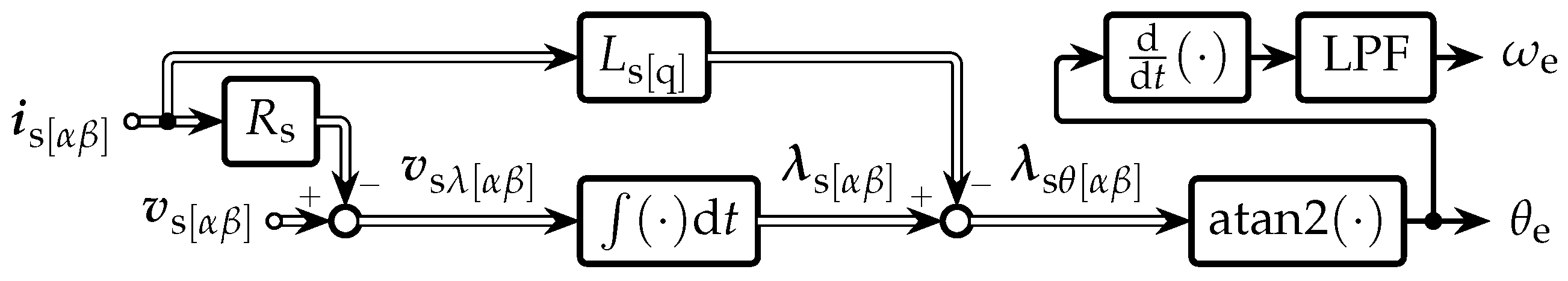
This way of expressing ${\theta }_{\mathrm{e}}$ and ${\omega }_{\mathrm{e}}$ eliminates the need for $L_{\mathrm{s}\left[\mathrm{d}\right]}$, which simplifies the observer that can be constructed based on Equations (19), (20) and (22) as it is shown by the diagram in Figure 1.

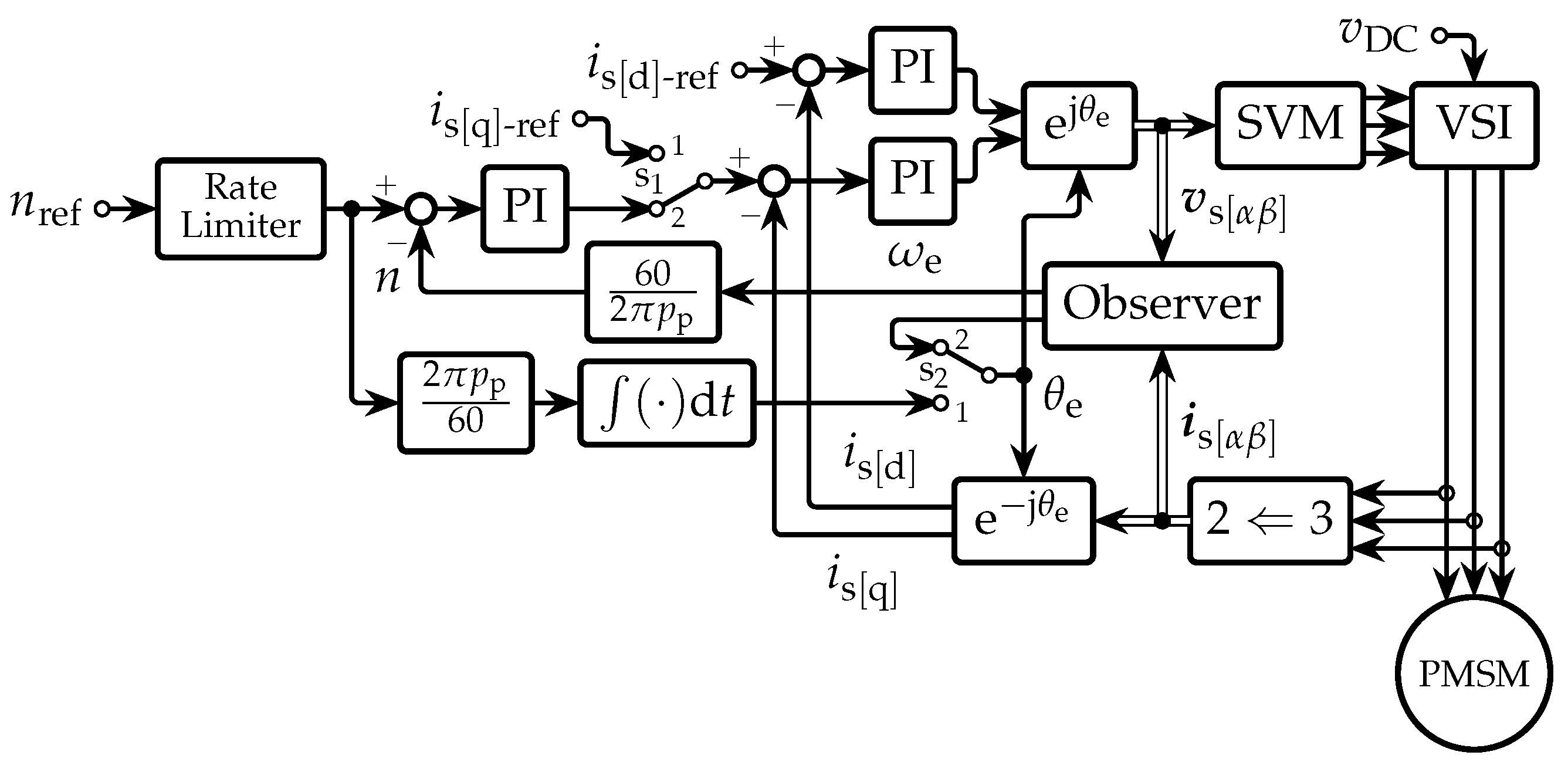
The simplicity and filtering properties of integration make this observer highly desirable and frequently used in selsorless applications of PMSMs whose examples can be found in [25,26,27,28], however, the drift caused by the integration represents the major obstacle in its practical implementations. In the case of significant changes in $R_{\mathrm{s}}$ that might be caused by extreme changes in temperature as well as in $L_{\mathrm{s}\left[\mathrm{q}\right]}$ that, depending on the design of the machine, might saturate by high currents, actual values of $R_{\mathrm{s}}$ and $L_{\mathrm{s}\left[\mathrm{q}\right]}$ can be estimated using the method described in [29]. The overall diagram of the sensorless FOC for PMSMs with a voltage source inverter (VSI) controlled by means of the space-vector modulation (SVM) that is regulated by proportional-integral controllers (PIs) is shown in Figure 2.

To initialize the sensorless FOC by the maximum of the electromagnetic torque ($T_{\mathrm{em}}$) for the reference of $i_{\mathrm{s}\left[\mathrm{q}\right]}$ ($i_{\mathrm{s}\left[\mathrm{q}\right]-\mathrm{ref}}$), ${\delta }_{\mathrm{e}}$ should optimally be ${90}^{\circ }$. Since ${\theta }_{\mathrm{e}}$ and the mechanical speed of the rotor (n) are initially unknown, the initialization of the control is performed by setting the switches ${\mathrm{s}}_1$ and ${\mathrm{s}}_2$ in the position 1 and the reference of $i_{\mathrm{s}\left[\mathrm{d}\right]}$ ($i_{\mathrm{s}\left[\mathrm{d}\right]-\mathrm{ref}}$) to the nominal value of the machine, while keeping $i_{\mathrm{s}\left[\mathrm{q}\right]-\mathrm{ref}}$ and the reference of n ($n_{\mathrm{ref}}$) at zero, until the direct axis of the rotor aligns with the magnetic axes of the stationary winding a. After the alignment of the rotor, $n_{\mathrm{ref}}$ is set to a desired value, based on which a forced value of ${\theta }_{\mathrm{e}}$ is generated. Simultaneously with $n_{\mathrm{ref}}$, $i_{\mathrm{s}\left[\mathrm{q}\right]-\mathrm{ref}}$ is set to the nominal value of the machine and $i_{\mathrm{s}\left[\mathrm{d}\right]-\mathrm{ref}}$ to zero. The rate limiter in Figure 2 ensures a controlled rise in $n_{\mathrm{ref}}$ until the value when the observer begins to generate values of ${\omega }_{\mathrm{e}}$ and ${\theta }_{\mathrm{e}}$. At that moment, the switches ${\mathrm{s}}_1$ and ${\mathrm{s}}_2$ are simultaneously set to the position 2 when the sensorless FOC is operational.

3. The Problem of the Drift

The drift can be defined as the accumulated offset caused by integration of an offset in the voltage represented by the integrand in Equation (22). Such an offset is primarily caused by initial conditions at transient states and additionally often by improperly calibrated shunts whose influence should be and typically is negligible. To present the problem in $\left[\alpha \beta \right]$, it is sufficient to consider ${\mathit{v}}_{\mathrm{s}\left[\alpha \beta \right]}$ and ${\mathit{i}}_{\mathrm{s}\left[\alpha \beta \right]}$ in a steady state. Therefore, ${\mathit{v}}_{\mathrm{s}\left[\alpha \beta \right]}$ with an offset can be defined in a steady state according to Equation (20) in terms of the magnitude of the zeroth harmonic of ${\mathit{v}}_{\mathrm{s}\left[\alpha \beta \right]}$ (${\mathit{v}}_{\mathrm{s}\left[\alpha \beta \right],0}$), which represents an offset in ${\mathit{v}}_{\mathrm{s}\left[\alpha \beta \right]}$, the magnitude of the fundamental harmonic of each voltage across each of the stationary windings ($v_{\mathrm{s},1}$), ${\omega }_{\mathrm{e}}$, ${\delta }_{\mathrm{e}}$, and the angular shift in the phase of ${\mathit{i}}_{\mathrm{s}}$ with respect to ${\mathit{v}}_{\mathrm{s}}$ (${\varphi }_i$) as

$$\begin{array}{ccc}\hfill {\mathit{v}}_{\mathrm{s}\left[\alpha \beta \right]}\left(t\right)& =& {\mathit{v}}_{\mathrm{s}\left[\alpha \beta \right],0}+v_{\mathrm{s},1}{\mathrm{e}}^{\mathrm{j}({\omega }_{\mathrm{e}}t+{\delta }_{\mathrm{e}}-{\varphi }_i)}.\hfill \end{array}$$

(23)

Similarly, ${\mathit{i}}_{\mathrm{s}\left[\alpha \beta \right]}$ with an offset can be defined in a steady state based on Equation (2) by adding the magnitude of the zeroth harmonic of ${\mathit{i}}_{\mathrm{s}\left[\alpha \beta \right]}$ (${\mathit{i}}_{\mathrm{s}\left[\alpha \beta \right],0}$), which represents an offset in ${\mathit{i}}_{\mathrm{s}\left[\alpha \beta \right]}$, and replacing ${\theta }_{\mathrm{e}}$ according to Equation (20) by ${\omega }_{\mathrm{e}}t$ as

$$\begin{array}{ccc}\hfill {\mathit{i}}_{\mathrm{s}\left[\alpha \beta \right]}\left(t\right)& =& {\mathit{i}}_{\mathrm{s}\left[\alpha \beta \right],0}+i_{\mathrm{s},1}{\mathrm{e}}^{\mathrm{j}({\omega }_{\mathrm{e}}t+{\delta }_{\mathrm{e}})}.\hfill \end{array}$$

(24)

Based on Equations (23) and (24), the derivative of ${\mathit{\lambda }}_{\mathrm{s}\left[\alpha \beta \right]}$ with respect to t in Equation (4) can be expressed as

$$\begin{array}{ccc}\hfill \frac{\mathrm{d}}{\mathrm{d}t}{\mathit{\lambda }}_{\mathrm{s}\left[\alpha \beta \right]}\left(t\right)& =& {\mathit{v}}_{\mathrm{s}\left[\alpha \beta \right],0}+v_{\mathrm{s},1}{\mathrm{e}}^{\mathrm{j}({\omega }_{\mathrm{e}}t+{\delta }_{\mathrm{e}}-{\varphi }_i)}-R_{\mathrm{s}}\left({\mathit{i}}_{\mathrm{s}\left[\alpha \beta \right],0}+i_{\mathrm{s},1}{\mathrm{e}}^{\mathrm{j}({\omega }_{\mathrm{e}}t+{\delta }_{\mathrm{e}})}\right),\hfill \end{array}$$

(25)

whose integration from $t=0$ to $t=\infty$ results in

$$\begin{array}{ccc}\hfill {\mathit{\lambda }}_{\mathrm{s}\left[\alpha \beta \right]}\left(t\right)& =& -\mathrm{j}\frac{1}{{\omega }_{\mathrm{e}}}\left(v_{\mathrm{s},1}{\mathrm{e}}^{\mathrm{j}({\omega }_{\mathrm{e}}t+{\delta }_{\mathrm{e}}-{\varphi }_i)}-R_{\mathrm{s}}{i}_{\mathrm{s},1}{\mathrm{e}}^{\mathrm{j}({\omega }_{\mathrm{e}}t+{\delta }_{\mathrm{e}})}\right)+\left({\mathit{v}}_{\mathrm{s}\left[\alpha \beta \right],0}+R_{\mathrm{s}}{\mathit{i}}_{\mathrm{s}\left[\alpha \beta \right],0}\right)t+{\mathit{\lambda }}_{\mathrm{s}\left[\alpha \beta \right]}\left(0\right).\hfill \end{array}$$

(26)

From Equation (26) it can be seen that ${\mathit{v}}_{\mathrm{s}\left[\alpha \beta \right],0}$ and ${\mathit{i}}_{\mathrm{s}\left[\alpha \beta \right],0}$ over time cause a linear increase in ${\mathit{\lambda }}_{\mathrm{s}\left[\alpha \beta \right]}$ and together with the initial condition ${\mathit{\lambda }}_{\mathrm{s}\left[\alpha \beta \right]}\left(0\right)$ constitute the drift in ${\lambda }_{\mathrm{s}\left[\alpha \beta \right]}$.

3.1. A Solution to the Problem

By expressing the direct component of ${\mathit{v}}_{\mathrm{s}\left[\alpha \beta \right],0}$ ($v_{\mathrm{s}\left[\alpha \right],0}$) and the direct component of ${\mathit{i}}_{\mathrm{s}\left[\alpha \beta \right],0}$ ($i_{\mathrm{s}\left[\alpha \right],0}$) in Equation (25), ${\lambda }_{\mathrm{s}\left[\alpha \right]}$ is defined as

$$\begin{array}{ccc}\hfill \frac{\mathrm{d}}{\mathrm{d}t}{\lambda }_{\mathrm{s}\left[\alpha \right]}\left(t\right)& =& v_{\mathrm{s}\left[\alpha \right],0}+v_{\mathrm{s},1}\cos ({\omega }_{\mathrm{e}}t+{\delta }_{\mathrm{e}}-{\varphi }_i)-R_{\mathrm{s}}\left(i_{\mathrm{s}\left[\alpha \right],0}+i_{\mathrm{s},1}\cos ({\omega }_{\mathrm{e}}t+{\delta }_{\mathrm{e}})\right),\hfill \end{array}$$

(27)

while based on the quadrature component of ${\mathit{v}}_{\mathrm{s}\left[\alpha \beta \right],0}$ ($v_{\mathrm{s}\left[\beta \right],0}$) and the quadrature component of ${\mathit{i}}_{\mathrm{s}\left[\alpha \beta \right],0}$ ($i_{\mathrm{s}\left[\beta \right],0}$) in Equation (25), ${\lambda }_{\mathrm{s}\left[\beta \right]}$ is defined as

$$\begin{array}{ccc}\hfill \frac{\mathrm{d}}{\mathrm{d}t}{\lambda }_{\mathrm{s}\left[\beta \right]}\left(t\right)& =& v_{\mathrm{s}\left[\beta \right],0}+v_{\mathrm{s},1}\sin ({\omega }_{\mathrm{e}}t+{\delta }_{\mathrm{e}}-{\varphi }_i)-R_{\mathrm{s}}\left(i_{\mathrm{s}\left[\beta \right],0}+i_{\mathrm{s},1}\sin ({\omega }_{\mathrm{e}}t+{\delta }_{\mathrm{e}})\right).\hfill \end{array}$$

(28)

According to Equation (26), ${\lambda }_{\mathrm{s}\left[\alpha \right]}$ is defined as

$$\begin{array}{ccc}\hfill {\lambda }_{\mathrm{s}\left[\alpha \right]}\left(t\right)& =& \frac{1}{{\omega }_{\mathrm{e}}}\left(v_{\mathrm{s},1}\sin ({\omega }_{\mathrm{e}}t+{\delta }_{\mathrm{e}}-{\varphi }_i)-R_{\mathrm{s}}{i}_{\mathrm{s},1}\sin ({\omega }_{\mathrm{e}}t+{\delta }_{\mathrm{e}})\right)+\left(v_{\mathrm{s}\left[\alpha \right],0}-R_{\mathrm{s}}{i}_{\mathrm{s}\left[\alpha \right],0}\right)t+{\lambda }_{\mathrm{s}\left[\alpha \right]}\left(0\right),\hfill \end{array}$$

(29)

while ${\lambda }_{\mathrm{s}\left[\beta \right]}$ is defined as

$$\begin{array}{ccc}\hfill {\lambda }_{\mathrm{s}\left[\beta \right]}\left(t\right)& =& \frac{1}{{\omega }_{\mathrm{e}}}\left(R_{\mathrm{s}}{i}_{\mathrm{s},1}\cos ({\omega }_{\mathrm{e}}t+{\delta }_{\mathrm{e}})-v_{\mathrm{s},1}\cos ({\omega }_{\mathrm{e}}t+{\delta }_{\mathrm{e}}-{\varphi }_i)\right)+\left(v_{\mathrm{s}\left[\beta \right],0}-R_{\mathrm{s}}{i}_{\mathrm{s}\left[\beta \right],0}\right)t+{\lambda }_{\mathrm{s}\left[\beta \right]}\left(0\right),\hfill \end{array}$$

(30)

where ${\lambda }_{\mathrm{s}\left[\alpha \right]}\left(0\right)$ and ${\lambda }_{\mathrm{s}\left[\beta \right]}\left(0\right)$ are initial conditions. Since the trigonometric terms in Equations (28) and (29) differ only by the factor of ${\omega }_{\mathrm{e}}$, the components causing the drift in the voltage equivalent to the uncompensated derivative of ${\lambda }_{\mathrm{s}\left[\alpha \right]}$ with respect to t ($v_{\mathrm{s}\lambda \left[\alpha \right]}$) can be extracted and compensated by introducing the correction of the drift in ${\lambda }_{\mathrm{s}\left[\alpha \right]}$ expressed at the level of $v_{\mathrm{s}\lambda \left[\alpha \right]}$ ($v_{\mathrm{s}\lambda \left[\alpha \right]-\mathrm{corr}}$), which is adjustable by the gain of the compensation loop (k), in the form

$$\begin{array}{ccc}\hfill v_{\mathrm{s}\lambda \left[\alpha \right]-\mathrm{corr}}\left(t\right)& =& \left({\omega }_{\mathrm{e}}\left(t\right){\lambda }_{\mathrm{s}\left[\alpha \right]}\left(t\right)-\frac{\mathrm{d}}{\mathrm{d}t}{\lambda }_{\mathrm{s}\left[\beta \right]}\left(t\right)\right)k\mathrm{sgn}\left({\omega }_{\mathrm{e}}\left(t\right)\right).\hfill \end{array}$$

(31)

Similarly, the trigonometric terms in Equations (27) and (30) differ in their signs and by the factor of ${\omega }_{\mathrm{e}}$, thus, the components causing the drift in the voltage equivalent to the uncompensated derivative of ${\lambda }_{\mathrm{s}\left[\beta \right]}$ with respect to t ($v_{\mathrm{s}\lambda \left[\beta \right]}$) can be extracted and compensated by introducing the correction of the drift in ${\lambda }_{\mathrm{s}\left[\beta \right]}$ expressed at the level of $v_{\mathrm{s}\lambda \left[\beta \right]}$ ($v_{\mathrm{s}\lambda \left[\beta \right]-\mathrm{corr}}$), also adjustable by k, in the form

$$\begin{array}{ccc}\hfill v_{\mathrm{s}\lambda \left[\beta \right]-\mathrm{corr}}\left(t\right)& =& \left({\omega }_{\mathrm{e}}\left(t\right){\lambda }_{\mathrm{s}\left[\beta \right]}\left(t\right)+\frac{\mathrm{d}}{\mathrm{d}t}{\lambda }_{\mathrm{s}\left[\alpha \right]}\left(t\right)\right)k\mathrm{sgn}\left({\omega }_{\mathrm{e}}\left(t\right)\right).\hfill \end{array}$$

(32)

Hence, the compensated derivative of ${\lambda }_{\mathrm{s}\left[\alpha \right]}$ with respect to t is then obtained as

$$\begin{array}{ccc}\hfill \frac{\mathrm{d}}{\mathrm{d}t}{\lambda }_{\mathrm{s}\left[\alpha \right]}\left(t\right)& =& v_{\mathrm{s}\lambda \left[\alpha \right]}\left(t\right)-v_{\mathrm{s}\lambda \left[\alpha \right]-\mathrm{corr}}\left(t\right),\hfill \end{array}$$

(33)

while the compensated derivative of ${\lambda }_{\mathrm{s}\left[\beta \right]}$ with respect to t is

$$\begin{array}{ccc}\hfill \frac{\mathrm{d}}{\mathrm{d}t}{\lambda }_{\mathrm{s}\left[\beta \right]}\left(t\right)& =& v_{\mathrm{s}\lambda \left[\beta \right]}\left(t\right)-v_{\mathrm{s}\lambda \left[\beta \right]-\mathrm{corr}}\left(t\right).\hfill \end{array}$$

(34)

Due to causality, ${\omega }_{\mathrm{e}}$ needed for the proposed compensation cannot be obtained by Equation (20), instead, it needs to be calculated prior to the compensation. Thus, ${\omega }_{\mathrm{e}}$ is calculated based on $v_{\mathrm{s}\lambda \left[\alpha \right]}$ and $v_{\mathrm{s}\lambda \left[\beta \right]}$ as

$$\begin{array}{ccc}\hfill {\omega }_{\mathrm{e}}\left(t\right)& =& \frac{\mathrm{d}}{\mathrm{d}t}\mathrm{atan}2(v_{\mathrm{s}\lambda \left[\beta \right]}\left(t\right),v_{\mathrm{s}\lambda \left[\alpha \right]}\left(t\right))\hfill \end{array}$$

(35)

and as such is used instead of Equation (20) for the sensorless FOC. Since differentiation amplifies noise, it is practically always implemented in a cascade with an LPF. Thus, by expressing Equation (35) in the form of a transfer function in the Laplace domain in terms of the cut-off frequency of the low-pass filter for the filtering of ${\omega }_{\mathrm{e}}$ (${\omega }_{\mathrm{c}}$) as

$$\begin{array}{ccc}\hfill {\omega }_{\mathrm{e}}\left(s\right)& =& s\frac{{\omega }_{\mathrm{c}}}{s+{\omega }_{\mathrm{c}}}\mathcal{L}\left\{\mathrm{atan}2(v_{\mathrm{s}\lambda \left[\beta \right]}\left(t\right),v_{\mathrm{s}\lambda \left[\alpha \right]}\left(t\right))\right\},\hfill \end{array}$$

(36)

which can be rearranged to the form

$$\begin{array}{ccc}\hfill {\omega }_{\mathrm{e}}\left(s\right)& =& \frac{{\omega }_{\mathrm{c}}}{{\displaystyle 1+\frac{\phantom{(}{\omega }_{\mathrm{c}}}{s}}}\mathcal{L}\left\{\mathrm{atan}2(v_{\mathrm{s}\lambda \left[\beta \right]}\left(t\right),v_{\mathrm{s}\lambda \left[\alpha \right]}\left(t\right))\right\}\hfill \end{array}$$

(37)

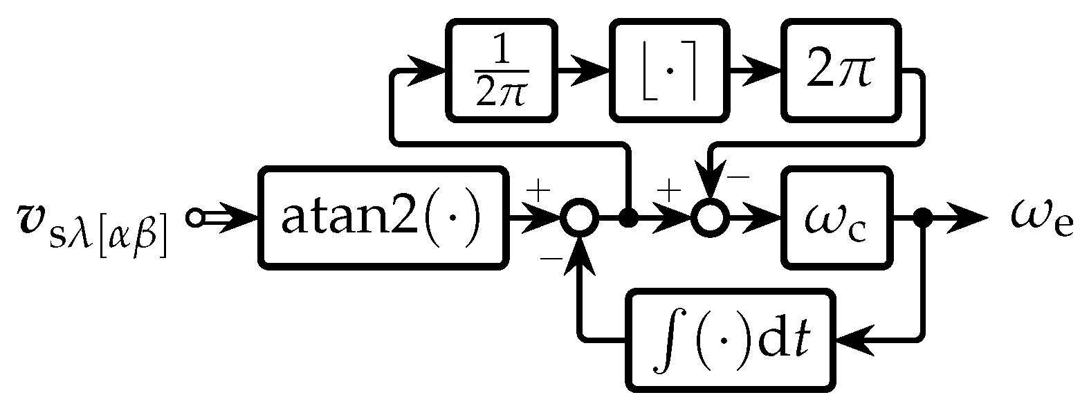
and observed as a closed-loop system, the observer of ${\omega }_{\mathrm{e}}$ can be constructed as it is shown in Figure 3. Moreover, based on the diagram in Figure 3, the observer of ${\omega }_{\mathrm{e}}$ can be expressed in the time domain as

$$\begin{array}{cc}\hfill {\omega }_{\mathrm{e}}\left(t\right)=& {\omega }_{\mathrm{c}}\stackrel{\mathrm{The}\mathrm{error}.}{\overbrace{[\mathrm{atan}2(v_{\mathrm{s}\lambda \left[\beta \right]}\left(t\right),v_{\mathrm{s}\lambda \left[\alpha \right]}\left(t\right))-\int {\omega }_{\mathrm{e}}\left(t\right)\mathrm{d}t}}\hfill \\ \hfill & \underset{\mathrm{The}\mathrm{wrapping}\mathrm{of}\mathrm{the}\mathrm{error}\mathrm{between}-\pi \mathrm{and}\pi .}{\underbrace{-2\pi ⌊\frac{1}{2\pi }\left(\mathrm{atan}2(v_{\mathrm{s}\lambda \left[\beta \right]}\left(t\right),v_{\mathrm{s}\lambda \left[\alpha \right]}\left(t\right))-\int {\omega }_{\mathrm{e}}\left(t\right)\mathrm{d}t\right)⌉]}},\hfill \end{array}$$

(38)

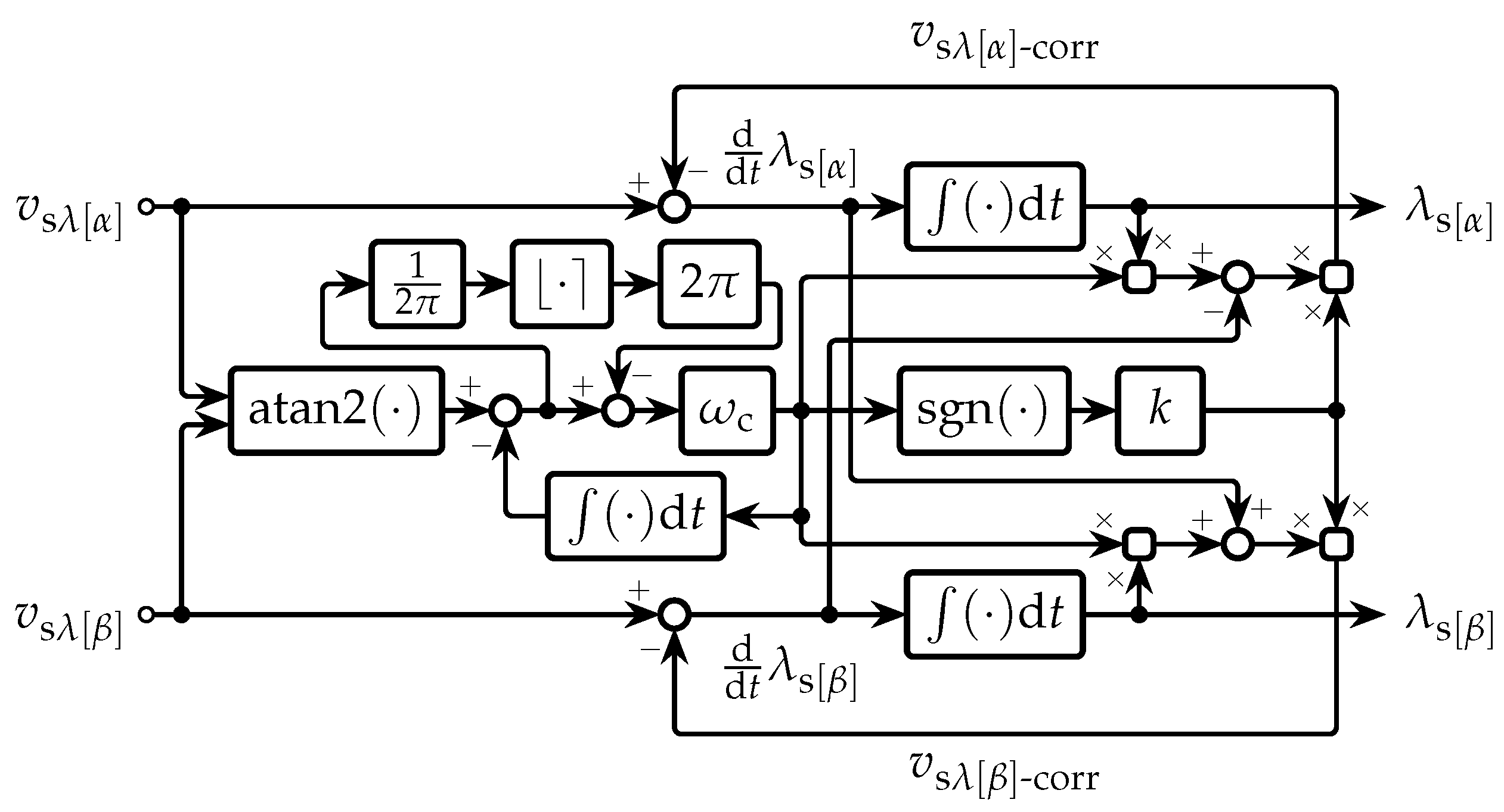
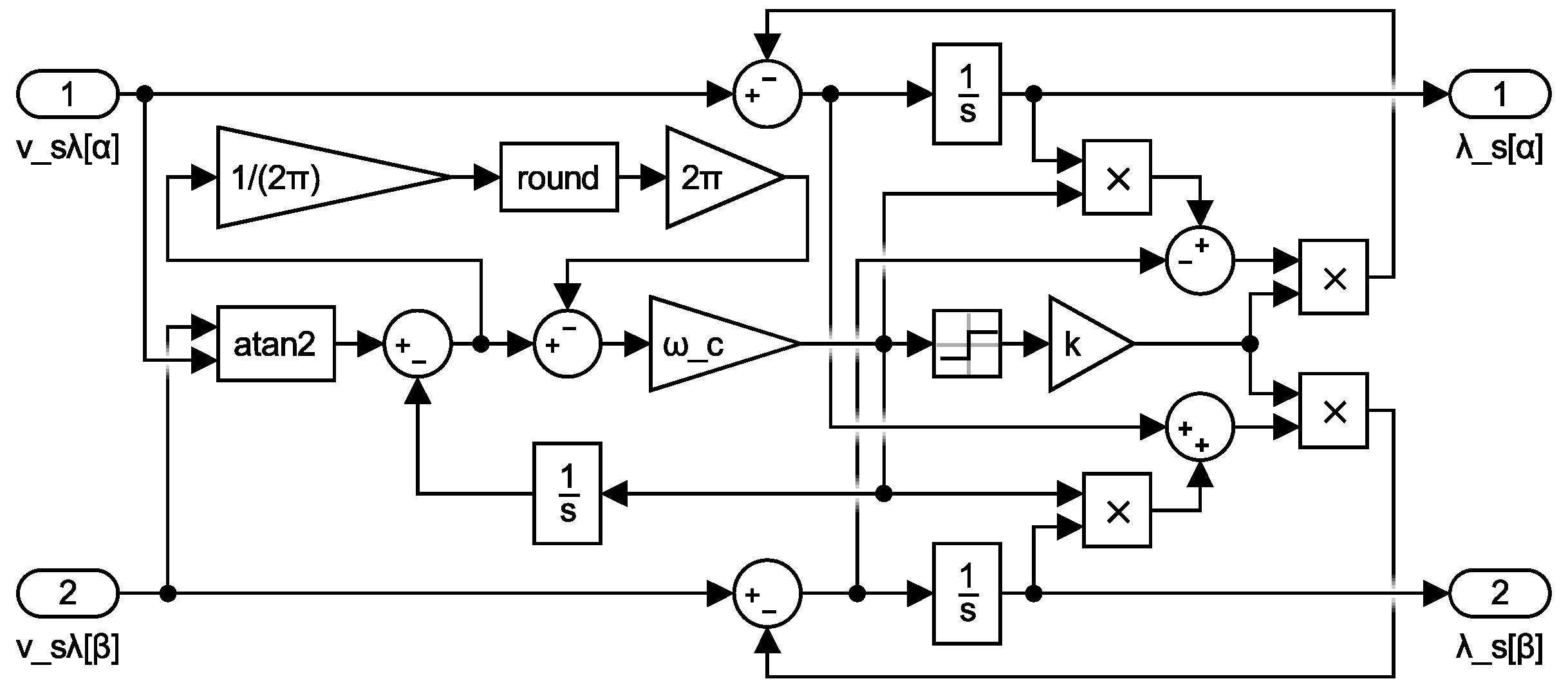
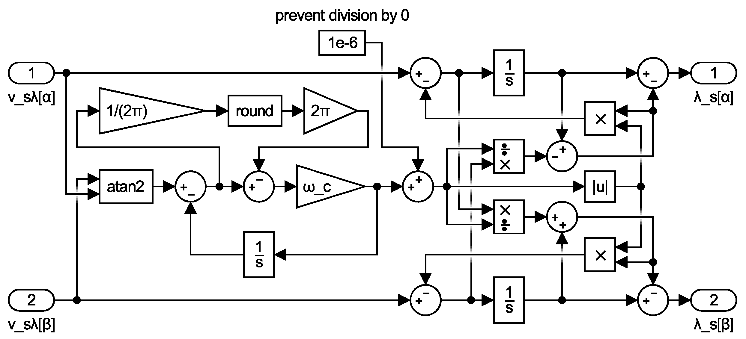
where the resulting error needs to be wrapped between $-\pi$ and $\pi$ to match the range of the four-quadrant inverse tangent function. The proposed compensation of the drift, presented by Equations (31)–(34) including Equation (38), represents a multiple input–multiple output (MIMO) phase-locked loop (PLL), which for an easier understanding is graphically presented by the diagram in Figure 4.

3.2. The Stability of the Proposed Compensation of the Drift

From Equations (31)–(34) it is obvious that the proposed compensation of the drift represents a nonlinear time-varying system that can be described by a pair of differential equations, namely

$$\begin{array}{ccc}\hfill \frac{\mathrm{d}}{\mathrm{d}t}{\lambda }_{\mathrm{s}\left[\alpha \right]}\left(t\right)& =& \frac{1}{k^2+1}\left(v_{\mathrm{s}\lambda \left[\alpha \right]}\left(t\right)-k\left|{\omega }_{\mathrm{e}}\left(t\right)\right|{\lambda }_{\mathrm{s}\left[\alpha \right]}\left(t\right)+k\mathrm{sgn}\left({\omega }_{\mathrm{e}}\left(t\right)\right)v_{\mathrm{s}\lambda \left[\beta \right]}\left(t\right)-k^2{\omega }_{\mathrm{e}}\left(t\right){\lambda }_{\mathrm{s}\left[\beta \right]}\left(t\right)\right),\hfill \end{array}$$

(39)

and

$$\begin{array}{ccc}\hfill \frac{\mathrm{d}}{\mathrm{d}t}{\lambda }_{\mathrm{s}\left[\beta \right]}\left(t\right)& =& \frac{1}{k^2+1}\left(v_{\mathrm{s}\lambda \left[\beta \right]}\left(t\right)-k\left|{\omega }_{\mathrm{e}}\left(t\right)\right|{\lambda }_{\mathrm{s}\left[\beta \right]}\left(t\right)-k\mathrm{sgn}\left({\omega }_{\mathrm{e}}\left(t\right)\right)v_{\mathrm{s}\lambda \left[\alpha \right]}\left(t\right)+k^2{\omega }_{\mathrm{e}}\left(t\right){\lambda }_{\mathrm{s}\left[\alpha \right]}\left(t\right)\right),\hfill \end{array}$$

(40)

where the nonlinearity defined by Equation (38) is represented by ${\omega }_{\mathrm{e}}$, which varies with t. Due to their specific structure, Equations (39) and (40) can be observed in a state-space as a linear parameter-varying system. Thus, by defining the state vector ($\mathbf{x}$) as

$$\begin{array}{ccc}\hfill \mathbf{x}\left(t\right)& =& \left[\begin{array}{c}{\lambda }_{\mathrm{s}\left[\alpha \right]}\left(t\right)\\ {\lambda }_{\mathrm{s}\left[\beta \right]}\left(t\right)\end{array}\right]\hfill \end{array}$$

(41)

and the input vector ($\mathbf{u}$) as

$$\begin{array}{ccc}\hfill \mathbf{u}\left(t\right)& =& \left[\begin{array}{c}{v}_{\mathrm{s}\lambda \left[\alpha \right]}\left(t\right)\\ v_{\mathrm{s}\lambda \left[\beta \right]}\left(t\right)\end{array}\right]\hfill \end{array}$$

(42)

as well as the state matrix ($\mathbf{A}$) as

$$\begin{array}{ccc}\hfill \mathbf{A}\left({\omega }_{\mathrm{e}}\left(t\right)\right)& =& \left[\begin{array}{cc}{\displaystyle -\frac{k|{\omega }_{\mathrm{e}}\left(t\right)|}{k^2+1}}& {\displaystyle -\frac{k^2{\omega }_{\mathrm{e}}\left(t\right)}{k^2+1}}\\ {\displaystyle \frac{k^2{\omega }_{\mathrm{e}}\left(t\right)}{k^2+1}}& {\displaystyle -\frac{k|{\omega }_{\mathrm{e}}\left(t\right)|}{k^2+1}}\end{array}\right]\hfill \end{array}$$

(43)

and the input matrix ($\mathbf{B}$) as

$$\begin{array}{ccc}\hfill \mathbf{B}\left({\omega }_{\mathrm{e}}\left(t\right)\right)& =& \left[\begin{array}{cc}{\displaystyle \frac{1}{k^2+1}}& {\displaystyle \frac{k\mathrm{sgn}\left({\omega }_{\mathrm{e}}\left(t\right)\right)}{k^2+1}}\\ {\displaystyle -\frac{k\mathrm{sgn}\left({\omega }_{\mathrm{e}}\left(t\right)\right)}{k^2+1}}& {\displaystyle \frac{1}{k^2+1}}\end{array}\right],\hfill \end{array}$$

(44)

the observed system can be presented in the state-space form

$$\begin{array}{ccc}\hfill \frac{\mathrm{d}}{\mathrm{d}t}\mathbf{x}\left(t\right)& =& \mathbf{A}\left({\omega }_{\mathrm{e}}\left(t\right)\right)\mathbf{x}\left(t\right)+\mathbf{B}\left({\omega }_{\mathrm{e}}\left(t\right)\right)\mathbf{u}\left(t\right).\hfill \end{array}$$

(45)

According to [30], the quadratic stability of the observed system for all uncertainties in ${\omega }_{\mathrm{e}}$, where ${\omega }_{\mathrm{e}}$ is bounded, can be proven in terms of a square matrix ($\mathbf{P}$) by constructing a quadratic Lyapunov function candidate ($\mathbf{V}$) in the form

$$\begin{array}{ccc}\hfill \mathbf{v}\left(\mathbf{x}\right(t\left)\right)& =& {\mathbf{x}}^{\mathrm{T}}\left(t\right)\mathbf{P}\mathbf{x}\left(t\right)\hfill \end{array}$$

(46)

so that a quadratic Lyapunov equation ($\mathbf{Q}$) fulfills the condition

$$\begin{array}{ccc}\hfill -\mathbf{Q}\left({\omega }_{\mathrm{e}}\left(t\right)\right)& =& {\mathbf{A}}^{\mathrm{T}}\left({\omega }_{\mathrm{e}}\left(t\right)\right)\mathbf{P}+\mathbf{P}\mathbf{A}\left({\omega }_{\mathrm{e}}\left(t\right)\right)<0,\hfill \end{array}$$

(47)

where

$$\begin{array}{ccc}\hfill \mathbf{P}& =& {\mathbf{P}}^{\mathrm{T}}>0,\hfill \end{array}$$

(48)

which is only true if all leading principal minors of $\mathbf{P}$ are positive. Accordingly, $\mathbf{P}$ can be selected in the diagonal form, in which case the element in the first row and the first column of $\mathbf{P}$ ($P_{1,1}$) and the element in the second row and the second column of $\mathbf{P}$ ($P_{2,2}$) must be positive definite, thus

$$\begin{array}{ccc}\hfill \mathbf{P}& =& \left[\begin{array}{cc}{P}_{1,1}& 0\\ 0& P_{2,2}\end{array}\right].\hfill \end{array}$$

(49)

By substituting Equations (43) and (49) into Equation (47), the following inequality is obtained

$$\begin{array}{ccc}\hfill \left[\begin{array}{cc}{\displaystyle -\frac{2k|{\omega }_{\mathrm{e}}\left(t\right)|}{k^2+1}{P}_{1,1}}& {\displaystyle \frac{k^2{\omega }_{\mathrm{e}}\left(t\right)}{k^2+1}\left(P_{2,2}-P_{1,1}\right)}\\ {\displaystyle \frac{k^2{\omega }_{\mathrm{e}}\left(t\right)}{k^2+1}\left(P_{2,2}-P_{1,1}\right)}& {\displaystyle -\frac{2k|{\omega }_{\mathrm{e}}\left(t\right)|}{k^2+1}{P}_{2,2}}\end{array}\right]& <& 0,\hfill \end{array}$$

(50)

which is fulfilled if

$$\begin{array}{ccc}\hfill \det (-{\mathbf{Q}}_{1,1}\left({\omega }_{\mathrm{e}}\left(t\right)\right))& =& -{\displaystyle \frac{2k|{\omega }_{\mathrm{e}}\left(t\right)|}{k^2+1}}{P}_{1,1}<0\hfill \end{array}$$

(51)

and

$$\begin{array}{ccc}\hfill \det (-\mathbf{Q}\left({\omega }_{\mathrm{e}}\left(t\right)\right))& =& {\left(\frac{2k|{\omega }_{\mathrm{e}}\left(t\right)|}{k^2+1}\right)}^2{P}_{1,1}{P}_{2,2}-{\left[\frac{k^2{\omega }_{\mathrm{e}}\left(t\right)}{k^2+1}\left(P_{2,2}-P_{1,1}\right)\right]}^2>0.\hfill \end{array}$$

(52)

The first condition defined by Equation (51) is fulfilled if $k>0$ and ${\omega }_{\mathrm{e}}\ne 0$, while the second condition defined by Equation (52) is always fulfilled if $k\ne 0$, ${\omega }_{\mathrm{e}}\ne 0$, and $P_{1,1}=P_{2,2}$. Therefore, by choosing $P_{1,1}=P_{2,2}$, the system is quadratically stable for arbitrarily fast time-varying uncertainties in ${\omega }_{\mathrm{e}}$ if $k>0$ and ${\omega }_{\mathrm{e}}\ne 0$. The validity of these conditions can be checked by Equations (31) and (32), where if ${\omega }_{\mathrm{e}}=0$, then $v_{\mathrm{s}\lambda \left[\alpha \right]-\mathrm{corr}}=0$ and $v_{\mathrm{s}\lambda \left[\alpha \right]-\mathrm{corr}}=0$ because $\mathrm{sgn}\left(0\right)=0$, which according to Equations (33) and (34) cancels the proposed compensation. Hence, the condition ${\omega }_{\mathrm{e}}\ne 0$ ensures the existence of $v_{\mathrm{s}\lambda \left[\alpha \right]-\mathrm{corr}}$ and $v_{\mathrm{s}\lambda \left[\alpha \right]-\mathrm{corr}}$, while $\mathrm{sgn}\left({\omega }_{\mathrm{e}}\right)$ ensures the negative feedback in Equations (33) and (34). Similarly, $k=0$ cancels the proposed compensation, while $k<0$ turns the negative feedback into a positive feedback and therefore makes the system unstable. Thus, only $k>0$ preserves the negative feedback and the stability.

4. Results of Simulations of the Proposed Compensation

To demonstrate the standalone functionality of the proposed compensation of the drift, without the sensorless FOC and considerations of possible states of the drive, several simulations were made in Matlab/Simulink (R2016a, MathWorks Inc., Natick, MA, USA) using the diagram shown in Figure 5.

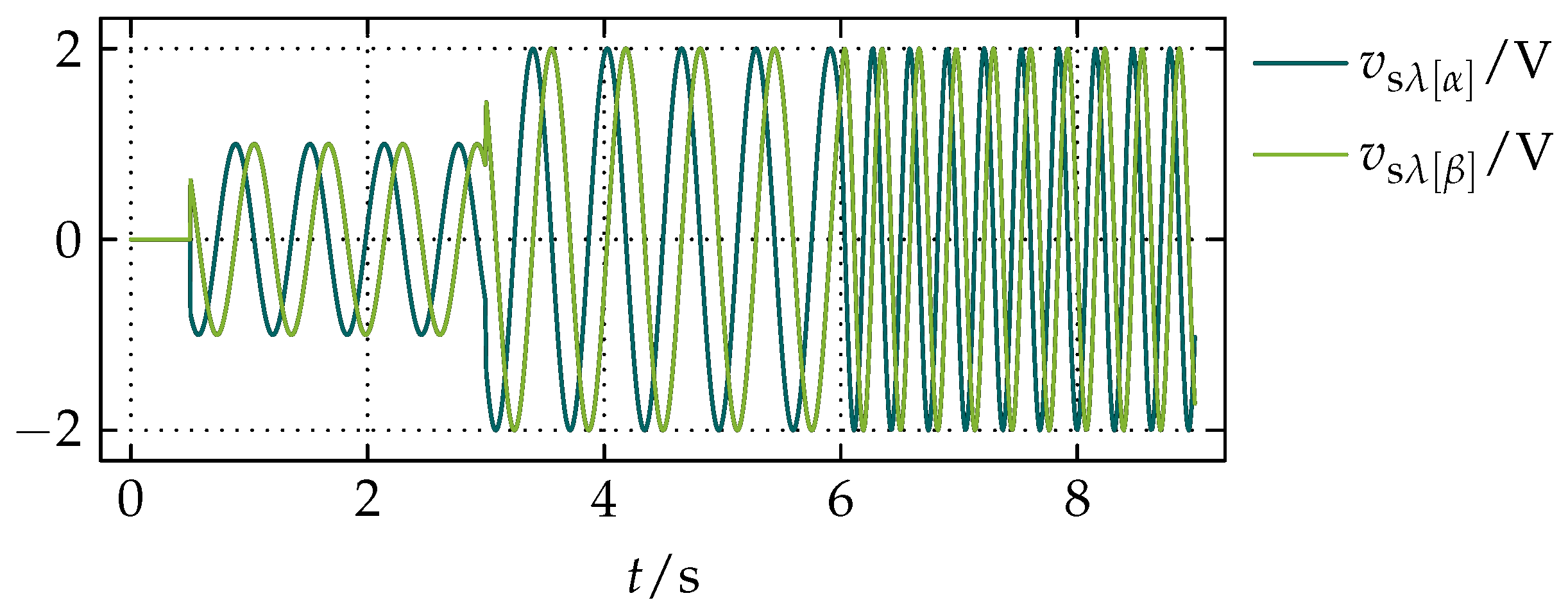
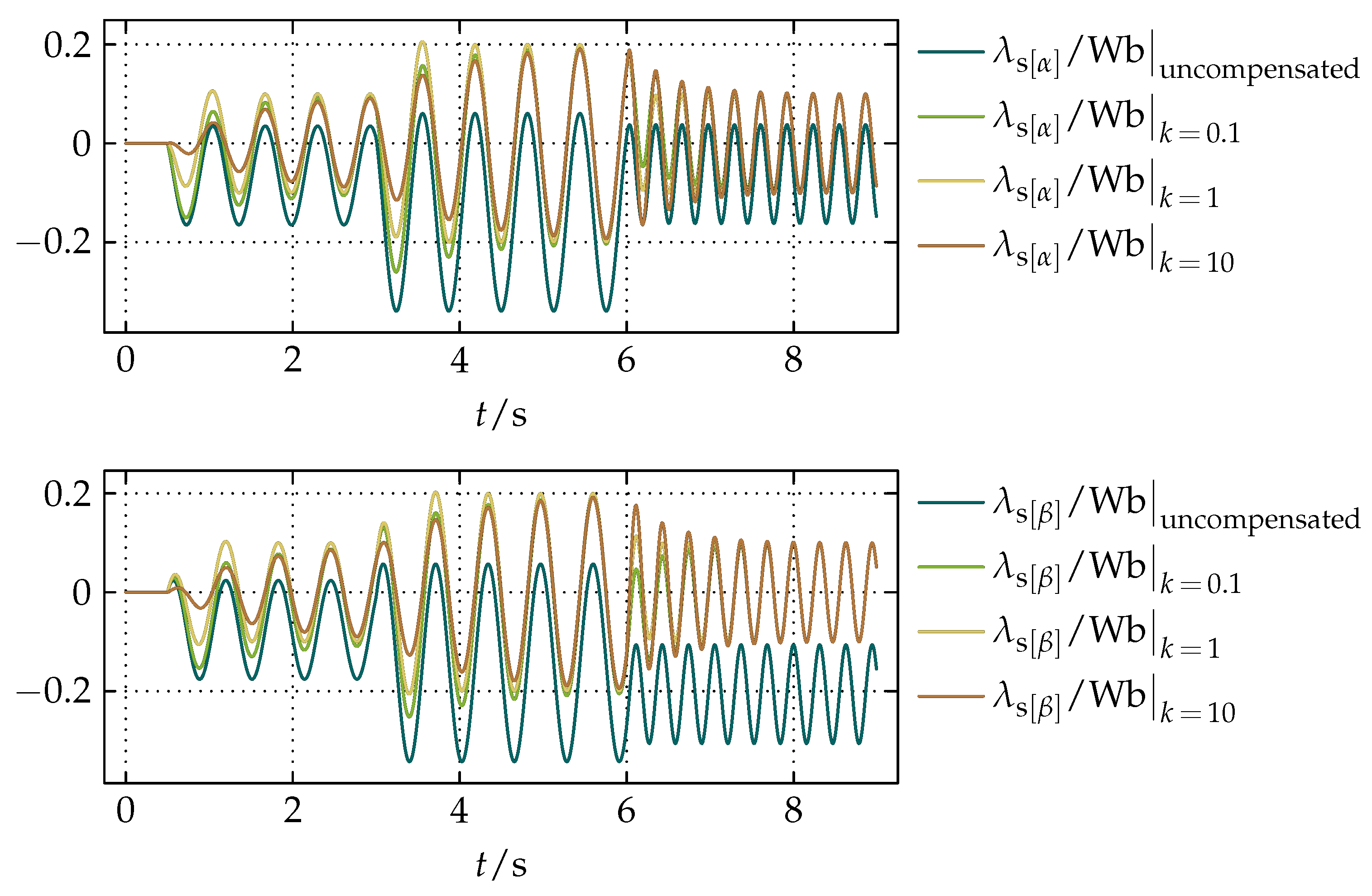
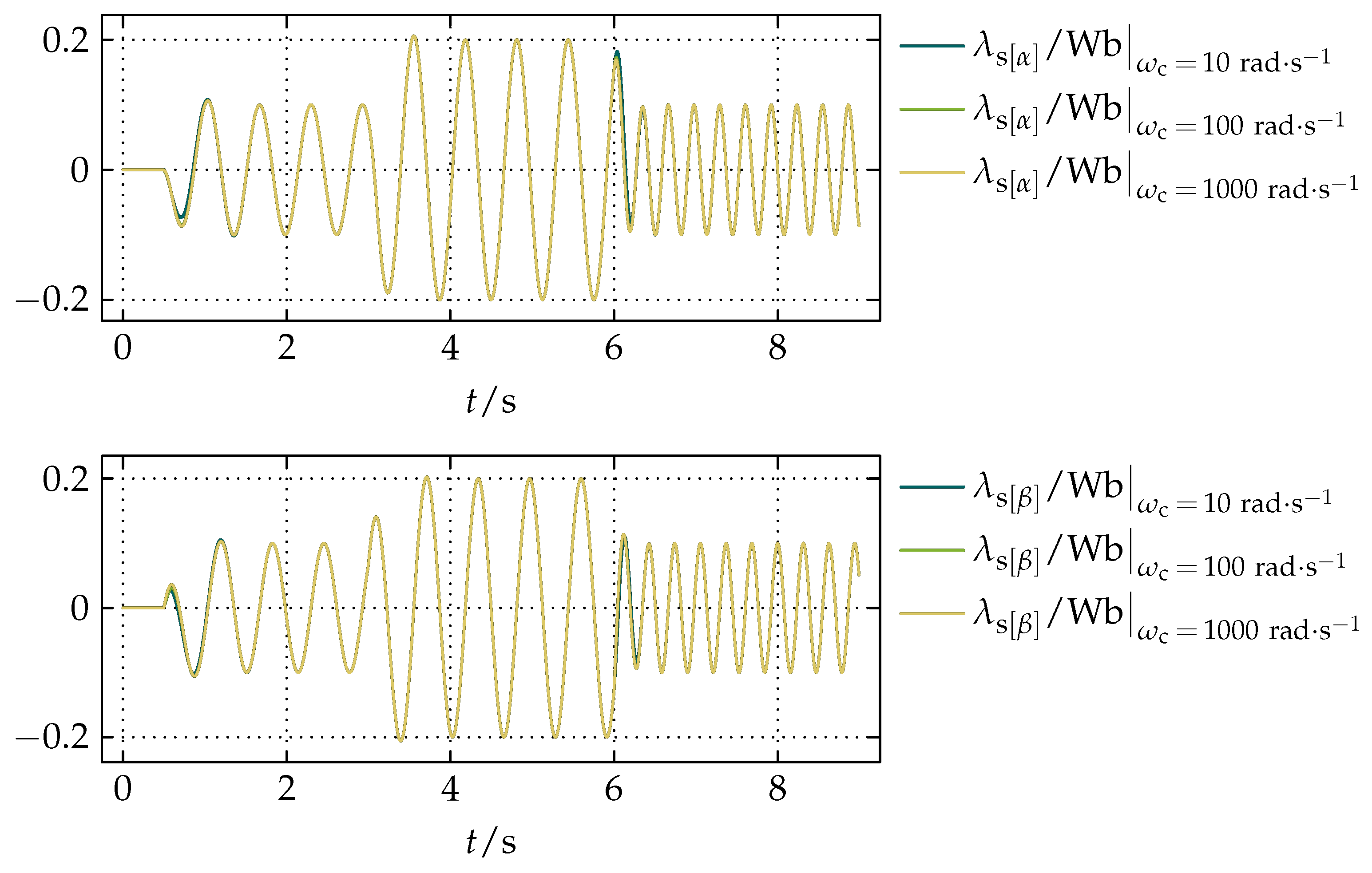
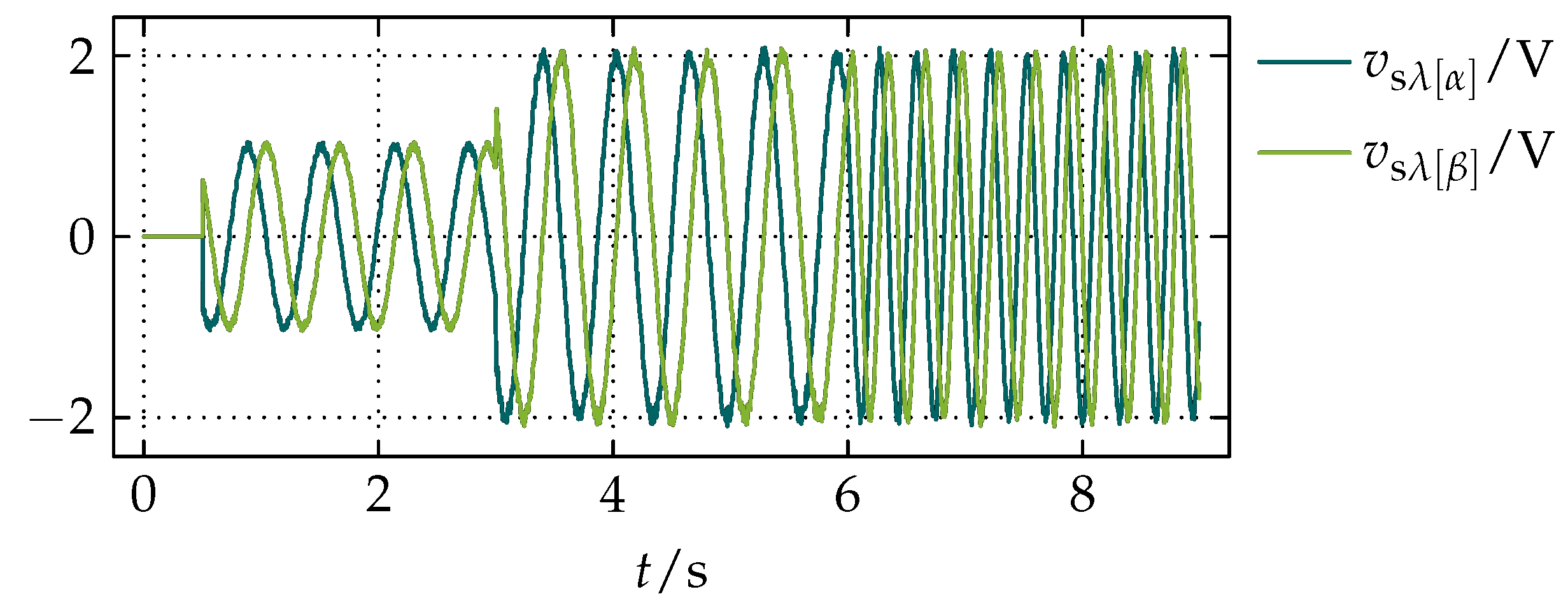
As test signals, the waveforms of $v_{\mathrm{s}\lambda \left[\alpha \right]}$ and $v_{\mathrm{s}\lambda \left[\beta \right]}$ were set to demonstrate the performance of the proposed compensation for changes in their magnitude and frequency. Thus, the initial magnitude from 0 to $0.5\mathrm{s}$ was set to $0\mathrm{V}$, from $0.5$ to $3\mathrm{s}$ was set to $1\mathrm{V}$, and from $3\mathrm{s}$ onward was set to $2\mathrm{V}$, while the frequency from 0 to $6\mathrm{s}$ was set to $10\mathrm{rad}·{\mathrm{s}}^{-1}$ and from $6\mathrm{s}$ onward was set to $20\mathrm{rad}·{\mathrm{s}}^{-1}$, as it is shown in Figure 6. The goal of the first simulation was to show the influence of k on the performance of the proposed compensation. The resulting waveforms of ${\lambda }_{\mathrm{s}\left[\alpha \right]}$ and ${\lambda }_{\mathrm{s}\left[\beta \right]}$ obtained for the constant value of ${\omega }_{\mathrm{c}}$ of $1000\mathrm{rad}·{\mathrm{s}}^{-1}$ and different values of k are shown in Figure 7. From Figure 7, it can be seen that values of k smaller than 1 result in overshoots in transient states whose settling time is longer for smaller values of k. Values of k greater than 1 produce undershoots whose settling time is longer for greater values of k. Hence, the value of k equal to 1 evidently provides the fastest response, that is, the shortest transient states. Based on that notion, the influence of variations in ${\omega }_{\mathrm{c}}$ is presented by the resulting waveforms of ${\lambda }_{\mathrm{s}\left[\alpha \right]}$ and ${\lambda }_{\mathrm{s}\left[\beta \right]}$ in Figure 8, where the value of k was set to 1 and ${\omega }_{\mathrm{c}}$ varied. From Figure 8, it can be noticed that variations in ${\omega }_{\mathrm{c}}$, or equivalently, changes in the bandwidth of the LPF for the filtering of ${\omega }_{\mathrm{e}}$ have a small influence on ${\lambda }_{\mathrm{s}\left[\alpha \right]}$ and ${\lambda }_{\mathrm{s}\left[\beta \right]}$ in transient states.

Results of Comparative Simulations of the Proposed Compensation and Referred Methods

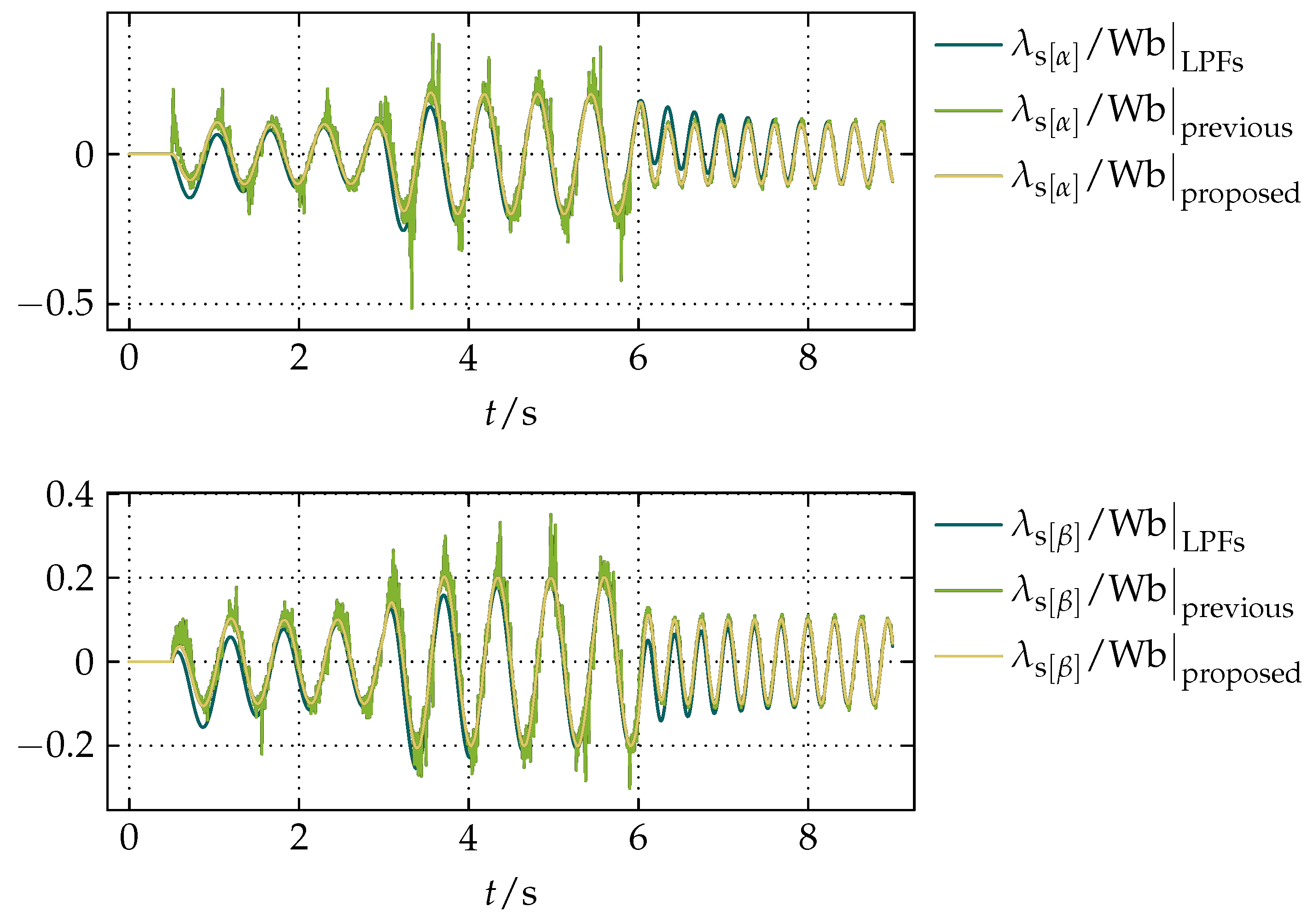
For qualitative comparisons of the proposed compensation with the state of the art, the standard solution with LPFs instead of the integrators presented in [5,6,7,8,9,10,11] was chosen as the first reference method, while the previous compensation introduced in [23] and presented by the diagram in Figure 9 was chosen as the second reference method.

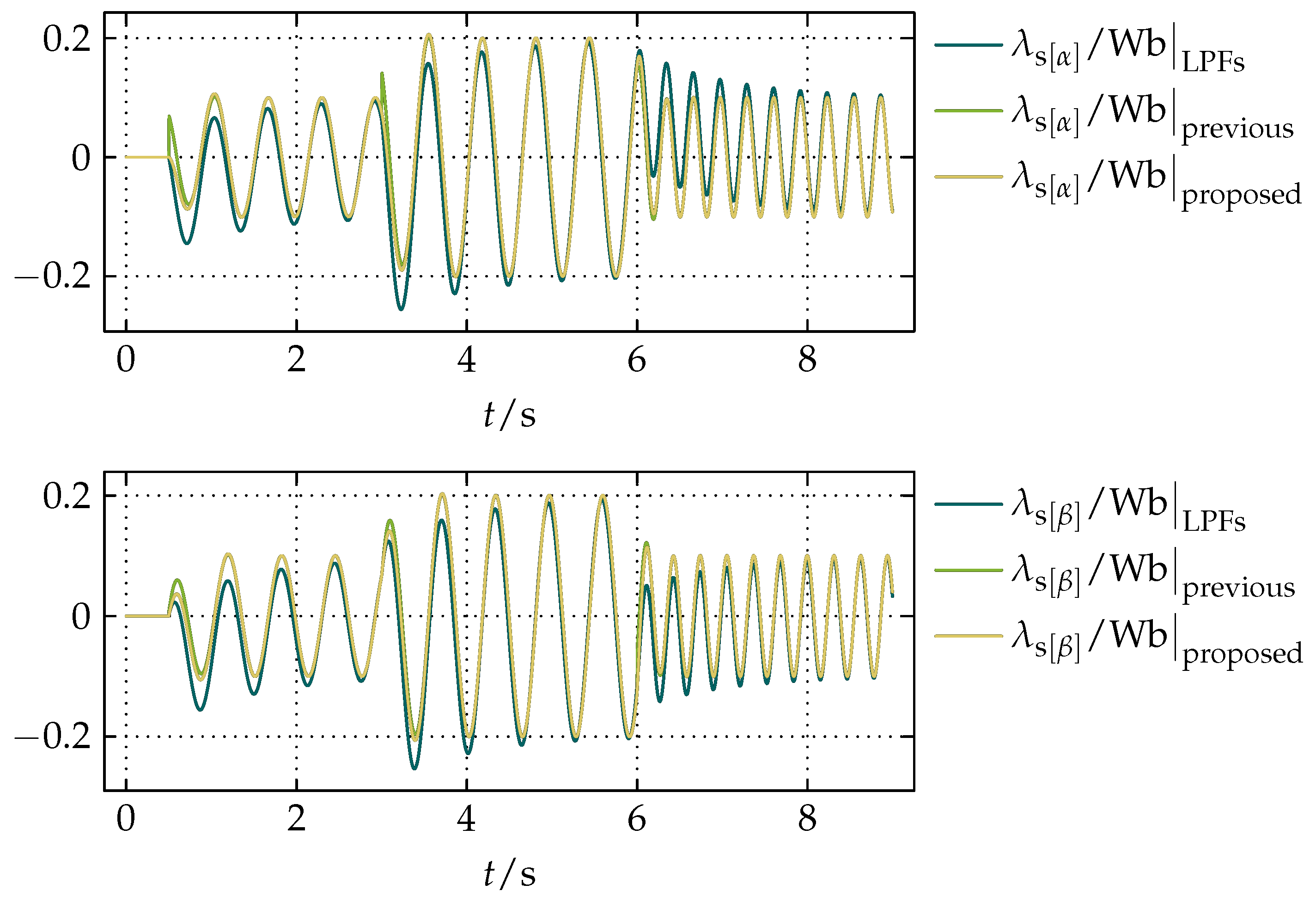
In the simulations, the cut-off frequencies of the LPFs in the first reference method were set to $1\mathrm{rad}·{\mathrm{s}}^{-1}$ to asymptotically match the magnitude characteristic of an integrator above $1\mathrm{rad}·{\mathrm{s}}^{-1}$ in the frequency domain. For the most unbiased comparison with the second reference method, k in the proposed compensation was set to 1 and ${\omega }_{\mathrm{c}}$ in both models was set to be equal, since the calculation of ${\omega }_{\mathrm{e}}$ in both models is the same. The resulting waveforms of ${\lambda }_{\mathrm{s}\left[\alpha \right]}$ and ${\lambda }_{\mathrm{s}\left[\beta \right]}$ to the same reference waveforms of $v_{\mathrm{s}\lambda \left[\alpha \right]}$ and $v_{\mathrm{s}\lambda \left[\beta \right]}$ in Figure 6 are shown in Figure 10.

The magnitude of ${\lambda }_{\mathrm{s}}$ ($|{\lambda }_{\mathrm{s}}|$) obtained as

$$\begin{array}{ccc}\hfill |{\lambda }_{\mathrm{s}}|\left(t\right)& =& \sqrt{\left({\lambda }_{\mathrm{s}\left[\alpha \right]}\left(t\right)\right){}^2+\left({\lambda }_{\mathrm{s}\left[\beta \right]}\left(t\right)\right){}^2}\hfill \end{array}$$

(53)

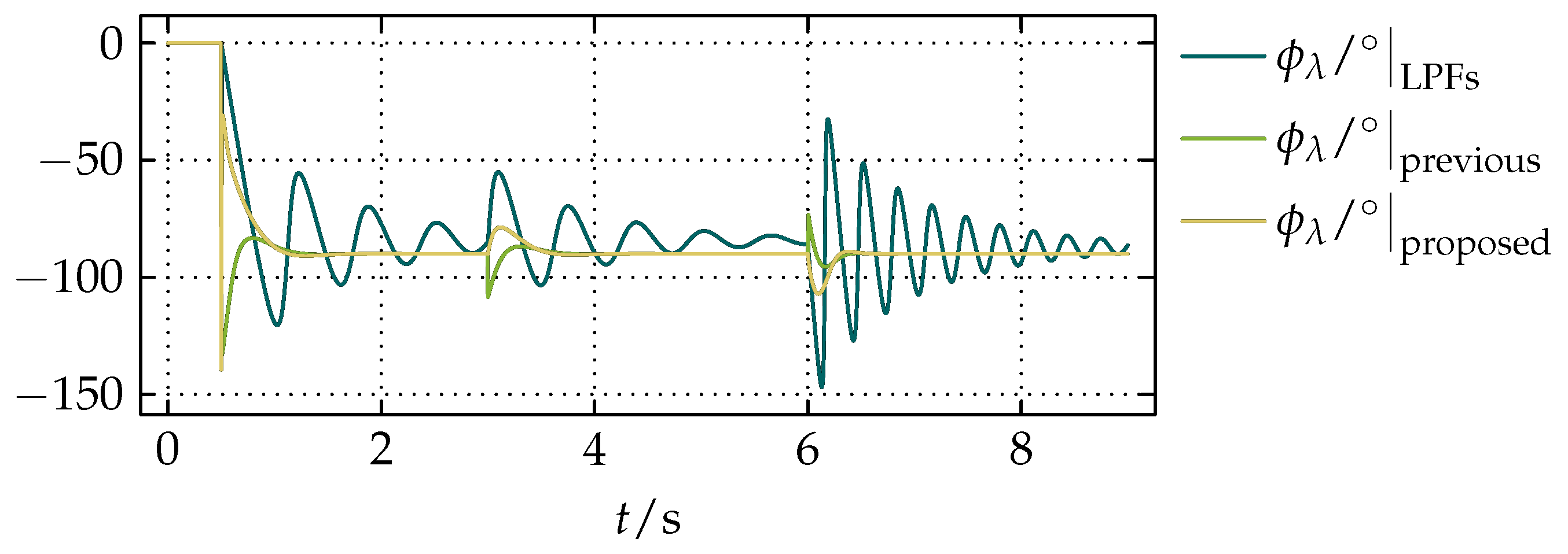
is shown in Figure 11, while the angular shift in the phase of ${\mathit{\lambda }}_{\mathrm{s}}$ with respect to the spatial phasor of the voltage equivalent to the uncompensated derivative of ${\mathit{\lambda }}_{\mathrm{s}}$ with respect to t (${\varphi }_{\lambda }$) is acquired as

$$\begin{array}{cc}\hfill {\varphi }_{\lambda }\left(t\right)=& \mathrm{atan}2({\lambda }_{\mathrm{s}\left[\beta \right]}\left(t\right),{\lambda }_{\mathrm{s}\left[\alpha \right]}\left(t\right))-\mathrm{atan}2(v_{\mathrm{s}\lambda \left[\beta \right]}\left(t\right),v_{\mathrm{s}\lambda \left[\alpha \right]}\left(t\right))\hfill \\ \hfill & -2\pi ⌊\frac{1}{2\pi }\left(\mathrm{atan}2({\lambda }_{\mathrm{s}\left[\beta \right]}\left(t\right),{\lambda }_{\mathrm{s}\left[\alpha \right]}\left(t\right))-\mathrm{atan}2(v_{\mathrm{s}\lambda \left[\beta \right]}\left(t\right),v_{\mathrm{s}\lambda \left[\alpha \right]}\left(t\right))\right)⌉\hfill \end{array}$$

(54)

and shown in Figure 12.

From the results presented in Figure 10, Figure 11 and Figure 12, it can be seen that the proposed compensation and the previous compensation presented in [23] have very similar settling times that are inversely proportional to ${\omega }_{\mathrm{e}}$ as well as significantly faster than the standard solution with LPFs. In Figure 12 it can be noticed that ${\varphi }_{\lambda }$ of both the proposed compensation and the previous compensation presented in [23] in the steady states is $-{90}^{\circ }$, as it is expected for integration, while for the standard solution with LPFs that is not the case. The proposed compensation has better filtering properties than the previous compensation in [23] due to its feedback-based structure, no discontinuities, and no divisions, which in fixed-point implementations on a DSP for small divisors can cause overflows and are generally more expensive than multiplications. To demonstrate the filtering properties, a random noise with the magnitude of $5\%$ of the magnitude of $v_{\mathrm{s}\lambda \left[\alpha \right]}$ and $v_{\mathrm{s}\lambda \left[\beta \right]}$ was added to them, which resulted in the noisy test signals shown in Figure 13.

The resulting waveforms of ${\lambda }_{\mathrm{s}\left[\alpha \right]}$ and ${\lambda }_{\mathrm{s}\left[\beta \right]}$ to the reference waveforms of $v_{\mathrm{s}\lambda \left[\alpha \right]}$ and $v_{\mathrm{s}\lambda \left[\beta \right]}$ in Figure 13 are shown in Figure 14, from which it can be noticed that the proposed compensation preserves the dynamic of the previous compensation in [23] while having the filtering properties of LPFs, but without any undesirable influence on $|{\lambda }_{\mathrm{s}}|$ and ${\varphi }_{\lambda }$ in steady states.

5. Results of Experiments of the Proposed Compensation within the Sensorless FOC of a PMSM

The practical functionality and the robustness of the proposed compensation was tested in the fixed-point 16-bit Q15 implementation within the Sensorless FOC of a PMSM on a MOSFET-based power electronics converter controlled by the Texas Instruments (Dallas, TX, USA) TM4C123BE microcontroller at the switching frequency of $10\mathrm{kHz}$. Parameters of the PMSM used in the experiments are listed in

Table 1. Parameters of the PMSM used in the experiments.

Parameter	Symbol	Value	Unit
DC-Link Voltage	$v_{\mathrm{DC}}$	24.00	V
Nominal Mechanical Speed	$n_{\mathrm{n}}$	4000.00	${\min }^{-1}$
Nominal Torque	$T_{\mathrm{n}}$	0.36	$\mathrm{N}·\mathrm{m}$
Number of Pole Pairs	$p_{\mathrm{p}}$	2.00
Stator Resistance	$R_{\mathrm{s}}$	0.15	$\mathsf{\Omega }$
Direct Synchronous Inductance	$L_{\mathrm{s}\left[\mathrm{d}\right]}$	0.39	$\mathrm{mH}$
Quadrature Synchronous Inductance	$L_{\mathrm{s}\left[\mathrm{q}\right]}$	0.59	$\mathrm{mH}$
Rotor Flux Constant	${\lambda }_{\mathrm{m}}$	14.78	$\mathrm{mWb}$

.

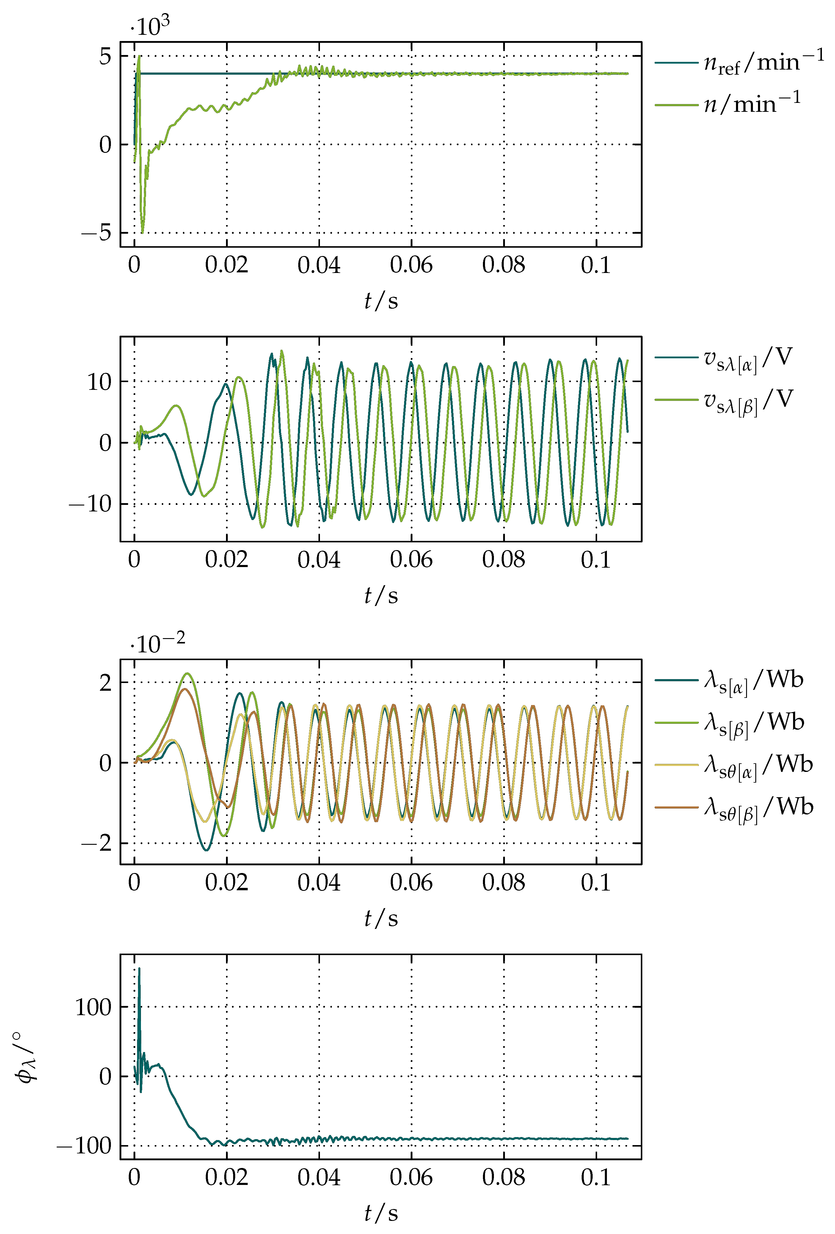
To test the speed of the convergence of the proposed compensation, a step in n from 0 to $4000{\min }^{-1}$ for $k=0.5$ and ${\omega }_{\mathrm{c}}$ matching the nominal electrical angular speed of the machine (${\omega }_{\mathrm{n}}$) was performed after the alignment of the rotor without any load and the initialization described at the end of Section 2.1. The results of that experiment are shown in Figure 15. Since each settling time in $|{\lambda }_{\mathrm{s}}|$ is equal to the corresponding one in ${\varphi }_{\lambda }$, as it is demonstrated in Figure 11 and Figure 12, ${\varphi }_{\lambda }$ can be taken as the measure of the speed of the convergence of the proposed compensation. Thus, from the plot of ${\varphi }_{\lambda }$ in Figure 15, it can be seen that the proposed compensation converges under $20\mathrm{ms}$, while the longer settling time of the magnitude of ${\lambda }_{\mathrm{s}\theta \left[\alpha \right]}$ and ${\lambda }_{\mathrm{s}\theta \left[\beta \right]}$, which corresponds to ${\lambda }_{\mathrm{m}}$ in Table 1 since $i_{\mathrm{s}\left[\mathrm{d}\right]-\mathrm{ref}}$ was kept zero, is imposed by the rest of the control system. It should also be noticed that $|{\lambda }_{\mathrm{s}}|$ is proportional to the quotient of the magnitude of $v_{\mathrm{s}\lambda \left[\alpha \right]}$ and $v_{\mathrm{s}\lambda \left[\beta \right]}$ ($|v_{\mathrm{s}\lambda }|$) and ${\omega }_{\mathrm{e}}$, where the relationship between ${\omega }_{\mathrm{e}}$ and n is defined in terms of the number of pole pairs ($p_{\mathrm{p}}$) as

$$\begin{array}{ccc}\hfill {\omega }_{\mathrm{e}}\left(t\right)& =& \frac{2\pi p_{\mathrm{p}}}{60}n\left(t\right).\hfill \end{array}$$

(55)

Although a startup from a standstill is possible, it is advisable to perform the initialization described at the end of Section 2.1 to avoid initial uncertainties and ensure a smooth start.

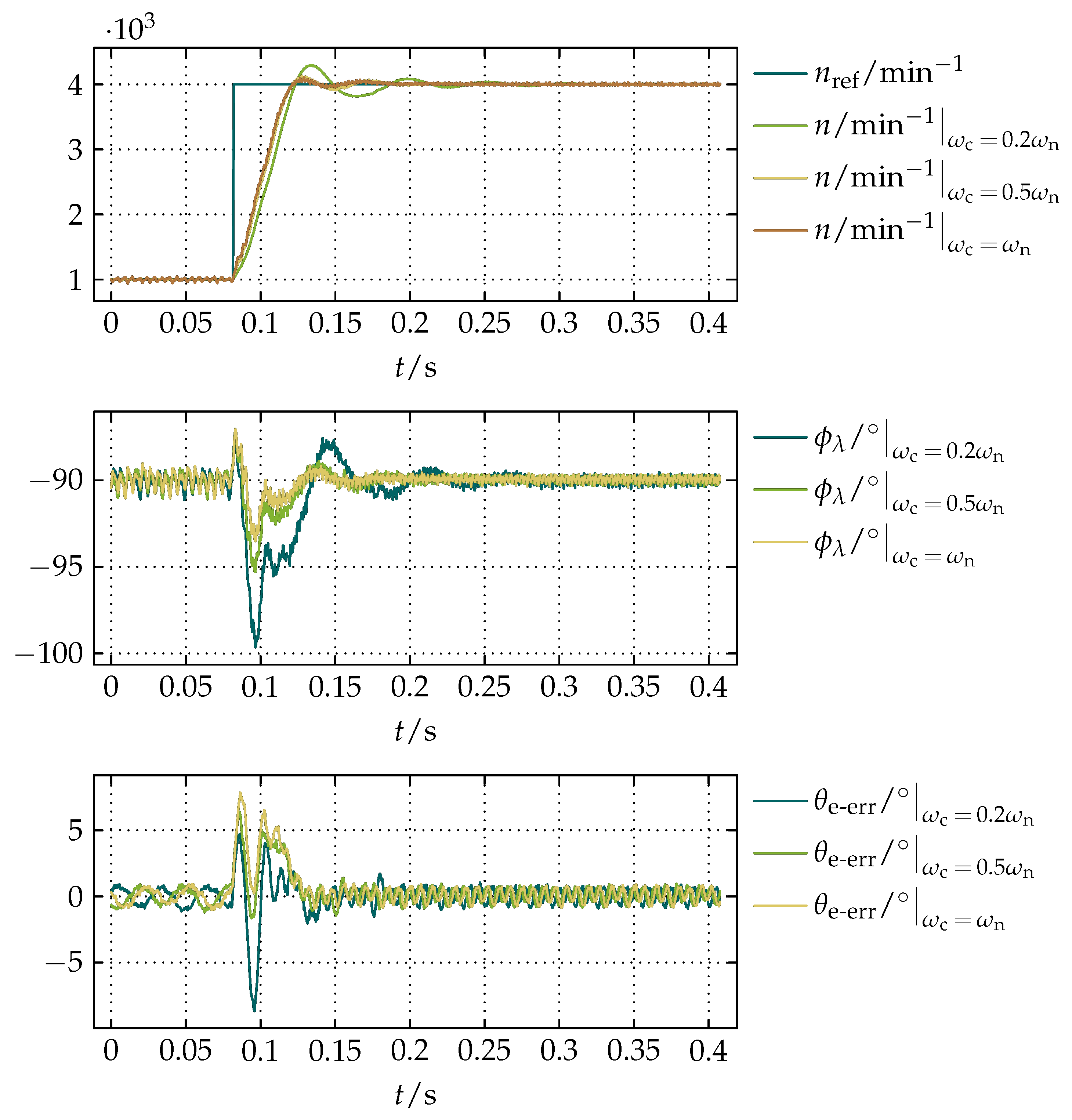
To demonstrate the influence of variations in ${\omega }_{\mathrm{c}}$ on the robustness of the proposed compensation and its influence on the sensorless FOC, three comparative experiments of a step in n from 1000 to $4000{\min }^{-1}$ for $k=0.5$ and varying ${\omega }_{\mathrm{c}}$ were performed. The results of those experiments are shown in Figure 16, where the error in ${\theta }_{\mathrm{e}}$ (${\theta }_{\mathrm{e}-\mathrm{err}}$) is expressed in terms of ${\theta }_{\mathrm{e}}$ and the actual electrical angular position of the rotor (${\theta }_{\mathrm{e}-\mathrm{act}}$) obtained by a position sensor as

$$\begin{array}{ccc}\hfill {\theta }_{\mathrm{e}-\mathrm{err}}\left(t\right)& =& {\theta }_{\mathrm{e}}\left(t\right)-{\theta }_{\mathrm{e}-\mathrm{act}}\left(t\right).\hfill \end{array}$$

(56)

From the results presented in Figure 16 it can be noticed that lower values of ${\omega }_{\mathrm{c}}$ result in higher overshoots and longer settling times for the same requirements of the sensorless FOC regarding the dynamics. However, overshoots can be reduced by reducing the dynamics of the sensorless FOC, which can be achieved by proportionally reducing the gains of the PIs in Figure 2.

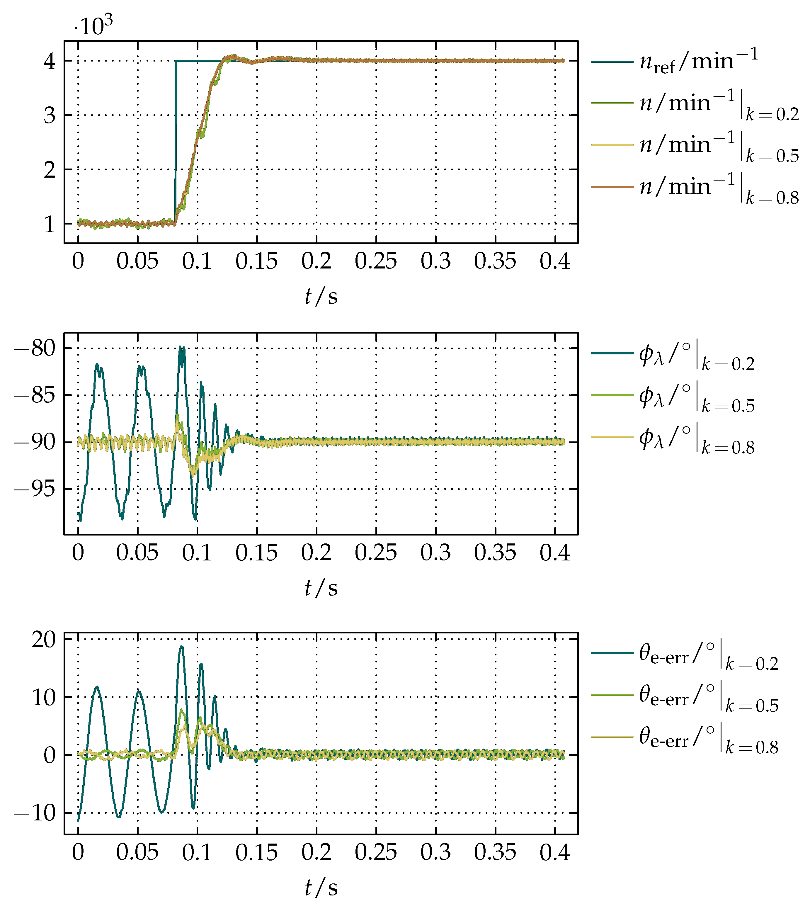
For the demonstration of the influence of variations in k on the robustness of the proposed compensation and its influence on the sensorless FOC, three additional comparative measurements of a step in n from 1000 to $4000{\min }^{-1}$ for ${\omega }_{\mathrm{c}}={\omega }_{\mathrm{n}}$ and varying k were done. From the results of those experiments presented in Figure 17, it can be noticed that k mostly influences the amount of oscillations in the system. Those oscillations become more noticeable for smaller values of k when $v_{\mathrm{s}\lambda \left[\alpha \right]-\mathrm{corr}}$ and $v_{\mathrm{s}\lambda \left[\beta \right]-\mathrm{corr}}$ are not sufficiently high enough to adequately compensate the drift. In addition, from the results of ${\varphi }_{\lambda }$ for $k=0.2$ in Figure 17, it can be noticed that at lower values of ${\omega }_{\mathrm{e}}$, or equivalently n, the magnitude of oscillations is greater because there is more time per an electric period for the accumulation of an offset that causes the drift and, consequently, oscillations.

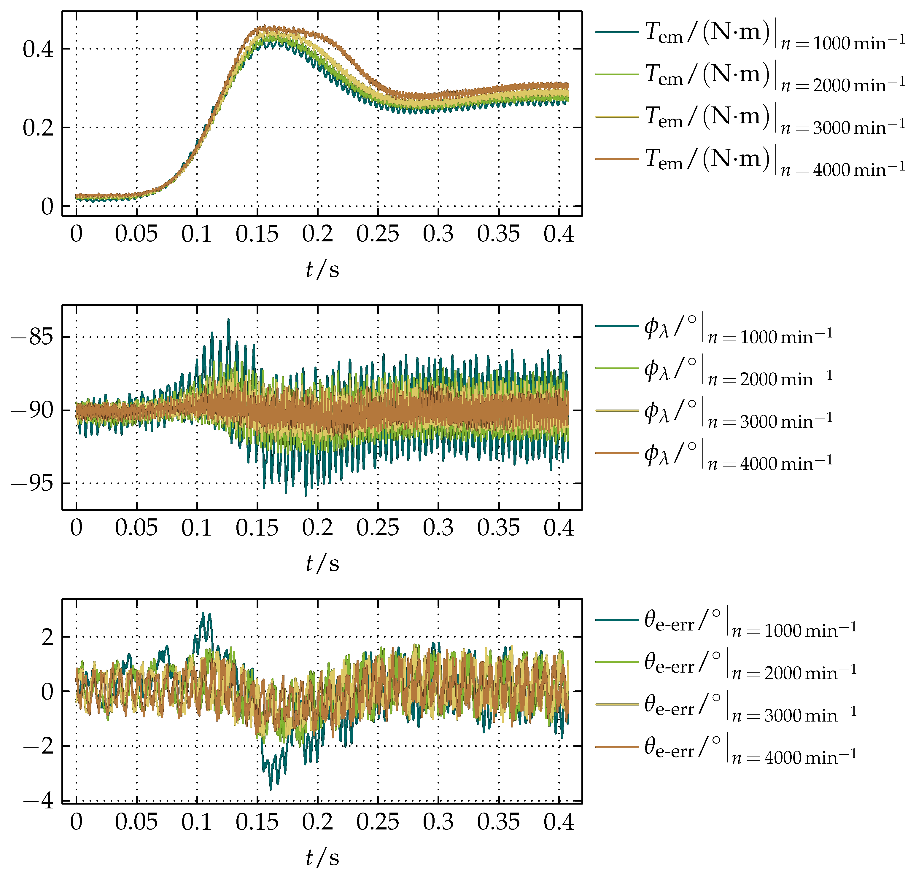
The robustness of the proposed compensation as well as its influence on the sensorless FOC during loading of the machine was tested by loading the machine with a hysteresis brake. Four comparative experiments for $k=0.5$ and ${\omega }_{\mathrm{c}}=0.2{\omega }_{\mathrm{n}}$ were carried out in the range of n from 1000 to $4000{\min }^{-1}$ in steps of $1000{\min }^{-1}$. From the resulting measurements shown in Figure 18, it can be seen that the machine was overloaded to about $125\%$ of the nominal torque ($T_{\mathrm{n}}$) listed in Table 1, whereby the peaks of the error in ${\varphi }_{\lambda }$ as well as in ${\theta }_{\mathrm{e}-\mathrm{err}}$ are more prominent at lower values of n because, as previously mentioned, there is more time per an electric period for the accumulation of an offset that causes the drift. Based on the presented results, it can be concluded that the error in ${\varphi }_{\lambda }$ and ${\theta }_{\mathrm{e}-\mathrm{err}}$ can be reduced by increasing k.

It is important to mention that the measured values of ${\theta }_{\mathrm{e}-\mathrm{act}}$ were used only as reference values for the evaluation of the performance of the proposed compensation within the sensorless FOC.

6. Conclusions

This paper has presented a simple self-contained solution that stems from the idea previously introduced in [23], which as such introduces improvements in the performance regarding fixed-point implementations on DSPs as well as filtering capabilities. The results of simulations presented in Section 4 have shown that the proposed compensation combines the dynamics of the previous solution proposed in [23] with the filtering properties of the standard solution with LPFs presented in [5,6,7,8,9,10,11]. Additionally, the results of experiments presented in Section 5 have confirmed the robustness of the proposed compensation and its functionality within the sensorless FOC.

In summary, the proposed compensation:

• is efficiently designed to be computationally suitable for inexpensive applications;
• for its operation requires only two periodic orthogonal input waveforms with a distinct common fundamental harmonic;
• is completely independent of the type and parameters of the used machine;
• provides correct values of $|{\lambda }_{\mathrm{s}}|$ and ${\varphi }_{\lambda }$ in steady states;
• has dynamics adjustable by ${\omega }_{\mathrm{c}}$ and k, which provide a fine-tuning without affecting $|{\lambda }_{\mathrm{s}}|$ and ${\varphi }_{\lambda }$ in steady states;
• can be used within the DTC and the sensorless FOC, or any other system that satisfies the requirement of orthogonality stated in the second point.

References

- Buja, G.S.; Kazmierkowski, M.P. Direct Torque Control of PWM Inverter-Fed AC Motors—A Survey. IEEE Trans. Ind. Electron. 2004, 51, 744–757. [Google Scholar] [CrossRef]
- Zhao, Y.; Zhang, Z.; Qiao, W.; Wu, L. An Extended Flux Model-Based Rotor Position Estimator for Sensorless Control of Salient-Pole Permanent-Magnet Synchronous Machines. IEEE Trans. Power Electron. 2015, 30, 4412–4422. [Google Scholar] [CrossRef]
- Holtz, J. Sensorless Control of Induction Motor Drives. Proc. IEEE 2002, 90, 1359–1394. [Google Scholar] [CrossRef]
- Seyoum, D.; Grantham, C.; Rahman, M.F. Simplified Flux Estimation for Control Application in Induction Machines. In Proceedings of the 2003 IEEE International Electric Machines and Drives Conference (IEMDC’03), Madison, WI, USA, 1–4 June 2003; pp. 691–695. [Google Scholar]
- Koteich, M. Flux Estimation Algorithms for Electric Drives: A Comparative Study. In Proceedings of the 2016 3rd International Conference on Renewable Energies for Developing Countries (REDEC), Zouk Mosbeh, Lebanon, 13–15 July 2016. [Google Scholar]
- Čolović, I.; Kutija, M.; Sumina, D. Rotor Flux Estimation for Speed Sensorless Induction Generator Used in Wind Power Application. In Proceedings of the 2014 IEEE International Energy Conference (ENERGYCON), Cavtat, Croatia, 13–16 May 2014; pp. 23–27. [Google Scholar]
- Pellegrino, G.; Bojoi, R.I.; Guglielmi, P. Unified Direct-Flux Vector Control for AC Motor Drives. IEEE Trans. Ind. Appl. 2011, 47, 2093–2102. [Google Scholar] [CrossRef] [Green Version]
- Idris, N.R.N.; Yatim, A.H.M. An Improved Stator Flux Estimation in Steady-State Operation for Direct Torque Control of Induction Machines. IEEE Trans. Ind. Appl. 2002, 38, 110–116. [Google Scholar] [CrossRef] [Green Version]
- Shen, J.X.; Hao, H.; Wang, C.F.; Jin, M.J. Sensorless Control of IPMSM Using Rotor Flux Observer. Int. J. Comput. Math. Electr. Electron. Eng. 2012, 32, 166–181. [Google Scholar] [CrossRef]
- Zhang, X.; Qu, W.; Lu, H. A New Integrator for Voltage Model Flux Estimation in a Digital DTC System. In Proceedings of the 2006 IEEE Region 10 Conference (TENCON 2006), Hong Kong, China, 14–17 November 2006. [Google Scholar]
- Xia, C.; Zhao, J.; Yan, Y.; Shi, T. A Novel Direct Torque Control of Matrix Converter-Fed PMSM Drives Using Duty Cycle Control for Torque Ripple Reduction. IEEE Trans. Ind. Electron. 2014, 61, 2700–2713. [Google Scholar] [CrossRef]
- Bose, B.K.; Patel, N.R. A Programmable Cascaded Low-Pass Filter-Based Flux Synthesis for a Stator Flux-Oriented Vector-Controlled Induction Motor Drive. IEEE Trans. Ind. Electron. 1997, 44, 140–143. [Google Scholar] [CrossRef]
- Norniella, J.G.; Cano, J.M.; Orcajo, G.A.; Rojas, C.H.; Pedrayes, J.F.; Cabanas, M.F.; Melero, M.G. Improving the Dynamics of Virtual-Flux-Based Control of Three-Phase Active Rectifiers. IEEE Trans. Ind. Electron. 2014, 61, 177–187. [Google Scholar] [CrossRef]
- Shin, M.H.; Hyun, D.S.; Cho, S.B.; Choe, S.Y. An Improved Stator Flux Estimation for Speed Sensorless Stator Flux Orientation Control of Induction Motors. IEEE Trans. Power Electron. 2000, 15, 312–318. [Google Scholar] [CrossRef]
- Zhang, Z.; Zhao, Y.; Qiao, W.; Qu, L. A Discrete-Time Direct-Torque and Flux Control for Direct-Drive PMSG Wind Turbines. In Proceedings of the 2013 IEEE Industry Applications Society Annual Meeting, Lake Buena Vista, FL, USA, 6–11 October 2013. [Google Scholar]
- Stojić, D.; Milinković, M.; Veinović, S.; Klasnić, I. Improved Stator Flux Estimator for Speed Sensorless Induction Motor Drives. IEEE Trans. Power Electron. 2014, 30, 2363–2371. [Google Scholar] [CrossRef]
- Hinkkanen, M.; Luomi, J. Modified Integrator for Voltage Model Flux Estimation of Induction Motors. IEEE Trans. Ind. Electron. 2003, 50, 818–820. [Google Scholar] [CrossRef]
- Hu, J.; Wu, B. New Integration Algorithms for Estimating Motor Flux over a Wide Speed Range. IEEE Trans. Power Electron. 1998, 13, 969–977. [Google Scholar] [CrossRef]
- Hurst, K.D.; Habetler, T.G.; Griva, G.; Profumo, F. Zero-Speed Tacholess IM Torque Control: Simply a Matter of Stator Voltage Integration. IEEE Trans. Ind. Appl. 1998, 34, 790–795. [Google Scholar] [CrossRef]
- Cho, K.R.; Seok, J.K. Pure-Integration-Based Flux Acquisition with Drift and Residual Error Compensation at a Low Stator Frequency. IEEE Trans. Ind. Appl. 2009, 45, 1276–1285. [Google Scholar] [CrossRef]
- Holtz, J. Sensorless Control of Induction Machines–with or without Signal Injection? IEEE Trans. Ind. Electron. 2006, 53, 7–30. [Google Scholar] [CrossRef]
- Holtz, J.; Quan, J. Drift- and Parameter-Compensated Flux Estimator for Persistent Zero-Stator-Frequency Operation of Sensorless-Controlled Induction Motors. IEEE Trans. Ind. Appl. 2003, 39, 1052–1060. [Google Scholar] [CrossRef]
- Strinić, T.; Silber, S.; Gruber, W. The Flux-Based Sensorless Field-Oriented Control of Permanent Magnet Synchronous Motors without Integrational Drift. Actuators 2018, 7, 35. [Google Scholar] [CrossRef]
- Krause, P.C.; Wasynczuk, O.; Sudhoff, S.D. Analysis of Electric Machinery and Drive Systems, 2nd ed.; John Wiley and Sons: New York, NY, USA, 2002; ISBN 0-471-14326-X. [Google Scholar]
- Imaeda, Y.; Doki, S.; Hasegawa, M.; Matsui, K.; Tomita, M.; Ohnuma, T. PMSM Position Sensorless Control with Extended Flux Observer. In Proceedings of the IECON 2011—37th Annual Conference of the IEEE Industrial Electronics Society, Melbourne, VIC, Australia, 7–10 November 2013. [Google Scholar]
- Boldea, I.; Paicu, M.C.; Andreescu, G.-D. Active Flux Concept for Motion-Sensorless Unified AC Drives. IEEE Trans. Power Electron. 2008, 23, 2612–2618. [Google Scholar] [CrossRef]
- Paicu, M.C.; Boldea, I.; Andreescu, G.-D.; Blaabjerg, F. Very Low Speed Performance of Active Flux Based Sensorless Control: Interior Permanent Magnet Synchronous Motor Vector Control versus Direct Torque and Flux Control. IET Electr. Power Appl. 2009, 3, 551–561. [Google Scholar] [CrossRef]
- Yuan, Q.; Yang, Z.-P.; Lin, F.; Sun, H. Sensorless Control of Permanent Magnet Synchronous Motor with Stator Flux Estimation. J. Comput. 2013, 8, 108–112. [Google Scholar] [CrossRef]
- Mercorelli, P. Parameters Identification in a Permanent Magnet Three-Phase Synchronous Motor of a City-Bus for an Intelligent Drive Assistant. Int. J. Model. Identif. Control 2014, 21, 352–361. [Google Scholar] [CrossRef]
- Hangos, K.M.; Bokor, J.; Szederkényi, G. Analysis and Control of Nonlinear Process Systems; Springer: London, UK, 2004; ISBN 1-85233-600-5. [Google Scholar]
Figure 1.
A diagram of the observer proposed for experiments, where is additionally filtered by an LPF.
Figure 2.
A simplified diagram of the sensorless FOC for PMSMs.
Figure 3.
A diagram of the proposed observer of .
Figure 4.
A diagram of the proposed compensation of the drift.
Figure 5.
The Simulink diagram of the proposed compensation used for simulations.
Figure 6.
The reference waveforms of and used as test signals for simulations.
Figure 7.
The resulting waveforms of and obtained by the simulation for and different values of k, including the uncompensated case equivalent to .
Figure 8.
The resulting waveforms of and obtained by a simulation for and different values of .
Figure 9.
The Simulink diagram of the previous compensation presented in [23] and used for comparative simulations.
Figure 10.
The resulting waveforms of and obtained by a comparative simulation of the standard solution with LPFs presented in [5,6,7,8,9,10,11], the previous compensation presented in [23], and the proposed compensation.
Figure 11.
The results of obtained by a comparative simulation of the standard solution with LPFs presented in [5,6,7,8,9,10,11], the previous compensation presented in [23], and the proposed compensation.
Figure 12.
Figure 13.
The reference waveforms of and used as noisy test signals for a simulation with disturbances.
Figure 14.
The resulting waveforms of and obtained by the simulation of the standard solution with LPFs presented in [5,6,7,8,9,10,11], the previous compensation presented in [23], and the proposed compensation, all with the noisy test signals.
Figure 15.
Results of an experiment of a step in n from 0 to for and .
Figure 16.
Results of comparative experiments of a step in n from 1000 to for and variations in .
Figure 17.
Results of comparative experiments of a step in n from 1000 to for and variations in k.
Figure 18.
Results of loading of the machine at 1000, 2000, 3000, and obtained by comparative experiments for and .