Article

A Novel Framework for a Systematic Integration of Pneumatic-Muscle-Actuator-Driven Joints into Robotic Systems Via a Torque Control Interface

1
Department of Electrical Engineering and Computer Science, Control Systems Group, Technical University of Berlin, Einsteinufer 17, D-10587 Berlin, Germany
2
Department VII, Electrical Engineering, Mechatronics and Optometry, Beuth Hochschule Berlin University of Applied Science, Luxemburger Straße 10, D-13353 Berlin, Germany
*
Author to whom correspondence should be addressed.
Actuators 2018, 7(4), 82; https://doi.org/10.3390/act7040082
Submission received: 7 November 2018 / Revised: 21 November 2018 / Accepted: 24 November 2018 / Published: 28 November 2018

Abstract

:
In this paper, two different torque control approaches for PMA-driven (PMA = Pneumatic muscle actuator) revolute joints are presented and tested. In previous work controllers for PMA-driven robots are typically customized for the use on a specific robotic system. In contrast, the proposed controllers define a general control interface for every robot that is actuated by PMA-driven joints. It will be shown that controlling the torque of a PMA-driven joint enables the use of standard robotic motion control frameworks, because the torque represents the natural input of the robotic equation of motion. Therefore, both proposed torque control approaches are interconnecting PMAs and their challenging characteristics on the one hand and “conventional” motion control strategies for robots on the other hand. After a detailed discussion of two different torque control approaches, we show that a torque controller handles all characteristics and dynamics of a PMA-driven joint internally, which implies that only its bandwidth and its static torque characteristic must be taken into account for the design of the outer motion control loop. This feature simplifies the integration of PMA-driven joints in robotic systems enormously, as will be demonstrated by a design of a cascade-structured, flatness-based motion controller for an exemplary robot with one degree of freedom.

1. Introduction

During the last decades, PMAs (PMA = Pneumatic muscle actuator, sometimes: PAM = Pneumatic artificial muscle) have been integrated in many robotic systems [1]. Especially in applications involving contact with human users, PMAs are particularly favored. The exoskeletons presented in [2,3], the rehabilitation robot in [4], the two-link, planar robot presented in [5], the two-degree-of-freedom parallel robot presented in [6,7] and the humanoid robot legs presented in [8] are only some examples of using PMAs in robotic systems. It is conspicuous that all of these robots have one thing in common: All of them are actuated only by PMA-driven joints.
After decades of investigating particular PMA-driven systems, the development of more systematic concepts for integrating PMAs in robotic systems is one of the latest interest of PMA research. In [9] a general design concept for antagonistic PMA-driven systems is given. This paper gives an excellent guidance on how to combine PMAs with respect to their static force map. However, since robots are dynamic systems, a static analysis on its own is not sufficient for controlling a PMA-driven robot.
Modelling and control of robotic systems is well described in the literature, see for example [10,11]. In the case of robots with only revolute joints, the equations of motion ([11] p. 271 ff) can be written in a slightly rearranged form
φ ¨ = M 1 ( φ ) τ h ( φ , φ ˙ ) ,
where τ is the joint torque and φ is the joint angle. The matrix M ( φ ) represents the system inertia and h ( φ , φ ˙ ) lumps together all centripetal, Coriolis, mass and friction terms [11]. The torque τ can be interpreted as the input and the vector ( φ , φ ˙ ) T as the state vector of the robotic system.
Although the theory of controlling robots is already well discussed, a general control framework for a systematic integration of PMA-driven joints in robotic systems is still missing and only control strategies for specific robots can be found in the literature. Taking a closer look at existing control strategies for robots driven by PMA-driven joints, all strategies can be mainly subdivided into two different groups. The first group is constituted by multiple-input-multiple-output (MIMO) controllers with state feedback, like the linear controller presented in [12] and the non-linear sliding mode controllers presented in [3,13]. Although it can be advantageous to control systems with a state feedback controller, the effort to design such a controller can be very high, especially if the system dynamics is non-linear like it is the case for PMA-driven joints. Alternatively, it is possible to split up the control problem in smaller sub-problems. This procedure leads to a cascade-structured controller, like it was e.g., implemented for a PMA-driven 2-DOF (DOF = degree of freedom) robotic system in [14]. This robot is controlled by an overlying motion controller that generates torque trajectories, while an underlying torque controller follows them. A similar cascade-structured controller was also used by [6,7] to control a two-degree-of-freedom parallel robot.
The idea to use an inner torque controller as an “interface” between PMAs on the one hand and the robotic equation of motion (1) on the other hand seems to be very intuitive. Provided that any joint is torque-controlled, the design of a cascade-structured motion controller based on the equation of motion is straight forward and can be done according to standard textbooks. Due to this, a general discussion of a torque controller for PMA-driven joints seems to be essential for a systematic integration of PMA-driven joints into new or even existing robotic systems. Nevertheless, to the best of our knowledge, there exists no general concept and thorough discussion of a torque controller for PMA-driven joints in the literature.
In the following paper a general discussion of two different torque controllers for PMA-driven joints will be given. After explaining the general structure of a PMA-driven joint, two variants of a torque controller for PMA-driven joints will be developed and discussed in Section 2. It will be shown that PMA-driven joints are completely defined by their static torque characteristic and their bandwidth. The second part of this paper will demonstrate how the two different torque controllers can simplify the integration of PMA-driven joints into an exemplary robotic system. A cascade-structured, flatness-based angular position controller for a 1-DOF robot will be designed in Section 3, in combination with either of both presented torque controllers.
Finally, it must be noted that the findings of the following text are not limited to the use on a specific robotic system; instead, they are shaping a general control interface for any robot which is actuated by PMA-driven joints.

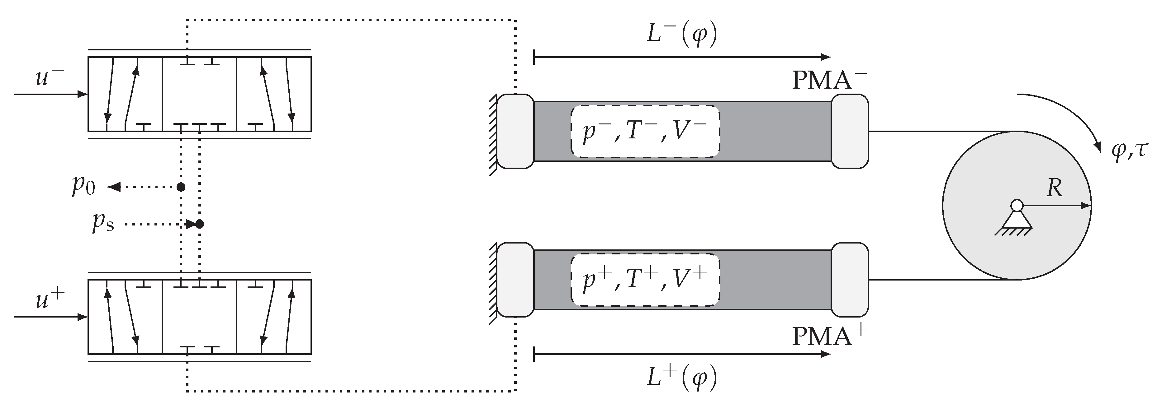
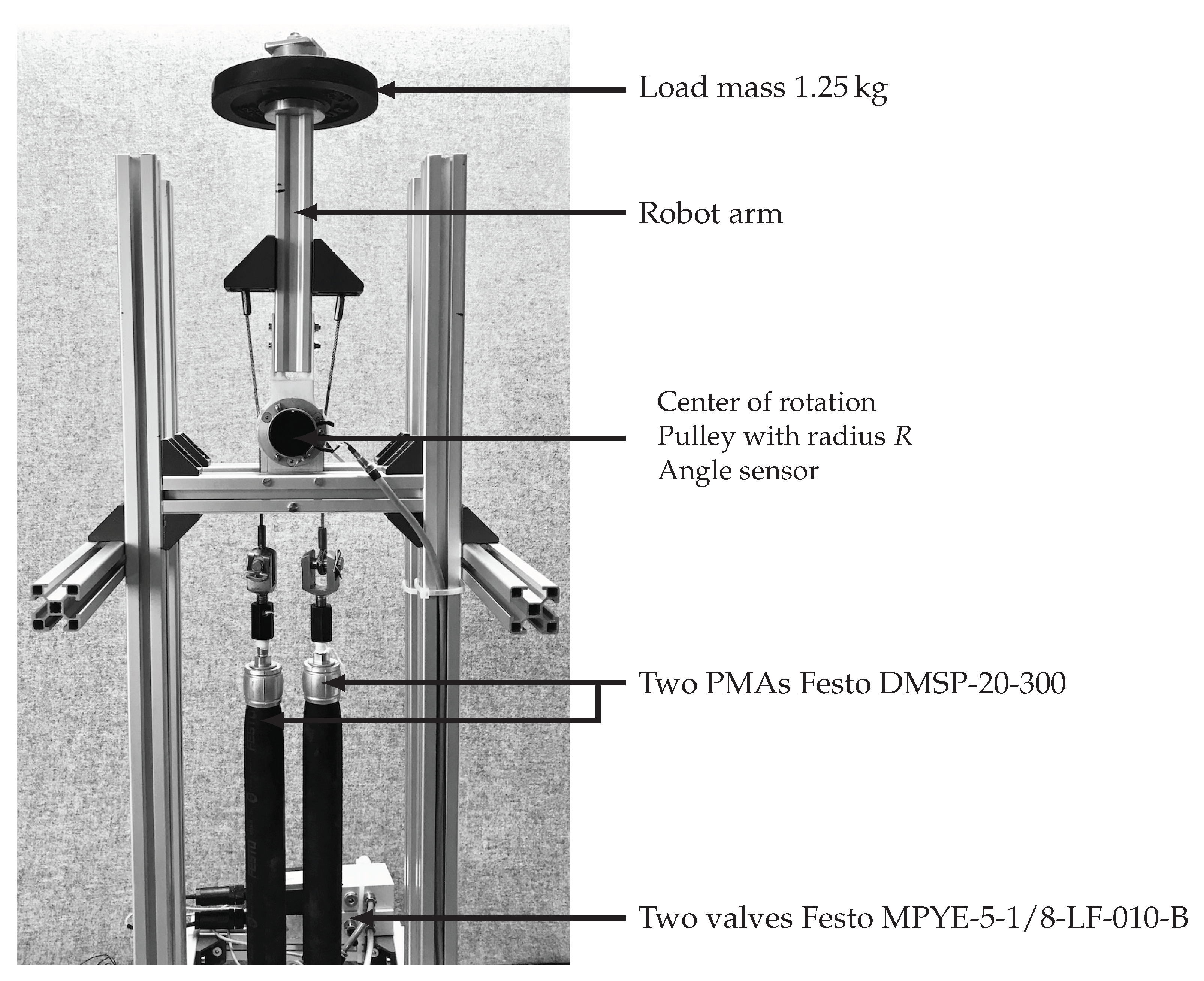
2. The PMA-Driven Joint

2.1. An Overview

A PMA-driven joint is a combination of two PMAs and a pulley with radius R, which can rotate around a fixed center. The rotation can be initiated by the PMAs, which are connected to the pulley via a rope or chain. As it can be seen in Figure 1, in this paper PMA + pulls in clockwise and PMA in counter-clockwise direction. Furthermore, the rotation-representing angle φ is defined to be positive for clockwise rotation and the radius is supposed to be constant.
The torque τ that the PMA-driven joint can exert is defined as the product of the pulley radius and the force difference.
τ PMA = R F PMA + F PMA
Due to the kinematic coupling of the PMA lengths, they are only a function of the pulley angle φ and given by
L + ( φ ) = L m R · φ and L ( φ ) = L m + R · φ .
The mean length L m is set to the length of half contraction, because this configuration leads to the widest angle range. Furthermore, the angle range is symmetric around φ = 0 , which represents the angle of the PMA-driven joint when both PMAs are half contracted.
As depicted in Figure 1, each PMA is controlled by a pneumatic valve. By changing the electrical control signal u ± either the supply pressure p s or the atmospheric pressure p 0 can be connected to the PMA. Due to this, the PMA pressure p ± , the PMA volume V ± and its temperature T ± are varying.
The creation of a torque controller for PMA-driven joints is the major goal of this paper. As depicted in Figure 2 the general structure of the torque controller is subdivided in a pressure trajectory generation and two pressure controllers, one for each PMA. The force difference between both PMAs defines a joint torque that the PMA-driven joint exerts. This is called a “sensor-less” approach [15] of a torque controller, because the torque is controlled without direct torque feedback.
It will be shown that only the definition of the pressure trajectories p ref ± limits the torque range that the PMA-driven joint is able to exert. Furthermore, it will be seen that the bandwidth of the torque controller is almost equal to the bandwidth of the pressure controllers.

2.2. Torque Characteristic

A precise model of the PMA forces is essential to control the torque of a PMA-driven joint. Several investigations of PMAs have shown, that the PMA force can be further subdivided into a static and a dynamic force. The latter, dynamic force is constituted by hysteresis [16,17] and some thermodynamic effects [18,19] and acts like a damper on the PMA-driven system [20]. Although measuring and compensating the dynamic PMA force and their effects is possible [21], the effort to do so is very high and the improvements are minor significant [17]. This implies that the static component dominates the PMA force. This statement gets emphasized by the excellent control results presented e.g., in [14,22,23,24] that were achieved only by modeling the PMA by its static force. Therefore, the influence of the dynamic PMA force will be generally neglected for this paper.
The main features of the static PMA force model presented in [25] are discussed briefly in Section 2.2.1. It will be seen that the PMA force F PMA ( p , L ) is a function of its pressure and length. With (2) in mind, the idea is to translate the torque trajectory into two PMA pressure trajectories. Obviously, this problem is underdefined, and therefore an additional algebraic constraint will be introduced. This additional constraint can be chosen in many different ways and will lead to a second equation such that the system of equations becomes solvable. A first variant of a constraint, discussed in Section 2.2.2, is given by the idea of a common mean pressure p m of both PMAs. This idea is the most popular constraint and was used e.g., in [14]. As an alternative approach, discussed in Section 2.2.3, it is possible to separate the torque in two PMA forces such that each force equation can be solved separately. This idea was first presented in [26].

2.2.1. PMA Force

As presented in [25], the static force characteristics of a Festo PMA (Festo Vertrieb GmbH & Co. KG, Esslingen a.N., Germany) is a function of its length L and pressure p, and can be described by
F PMA ( p , L ) = p · A ( L ) + B ( L ) .
The factors, denoted by A and B, can be explicitly written as
A ( L ) = L Fiber 2 3 L 2 4 π n 2 B ( L ) = π H 0 E RU ( L ) L 2 n π L Fiber 2 L 2 · D ( L ) D 0 D 0 L L 0 L 0 · D ( L ) ,
where
L Fiber = L 0 cos θ 0 and n = L 0 tan θ 0 π D 0 .
Although many other models can be found in the literature [14,19,25,27,28], (4) is most suitable (in the sense of the smallest deviation from the measured force map) to approximate the static PMA force [25]. The lower index 0, in (5), indicates the initial state of the PMA, with atmospheric pressure p 0 , initial rubber tube length L 0 , inner diameter D 0 and fiber angle θ 0 [25]. While the initial tube length and the inner diameter can be obtained easily, the initial fiber angle must be identified by solving the optimization problem presented in [25]. In the current paper a Festo DMSP-20-300 (DMSP - <initial inner diameter in millimeter> - <initial length in millimeter>) will be used for all experimental investigations. Following the procedure presented in [25,29], the initial fiber angle is identified as θ 0 ( D M S P 20 300 ) = 25.9952 ° for the DMSP-20-300. The factor H 0 ( 1.8 mm for a DMSP-20-300) represents the membrane thickness and is identified by measurement. Important to know is that the PMA volume
V ( L ) = L · L Fiber 2 4 π n 2 L 3 4 π n 2
as well as the PMA diameter
D ( L ) = L Fiber 2 L 2 n π
are only depending on the PMA length L [30]. This is the same for the modulus of elasticity
E RU ( L ) = c 3 L 3 + c 2 L 2 + c 1 L + c 0 ,
as is presented in [25]. The modulus of elasticity can be approximated by a third-order polynomial in L, where the parameters c 0 , 1 , 2 , 3 can be identified by the solving the optimization problem presented in [25]. Using the optimization start parameters from [25], the correct results for a DMSP-20-300 can be found in Table 1. The measured force map that is needed as a reference within the optimization process can be found in Appendix B.
The maximum error between (4) and the measured force map of a DMSP-20-300 is 3.55%.

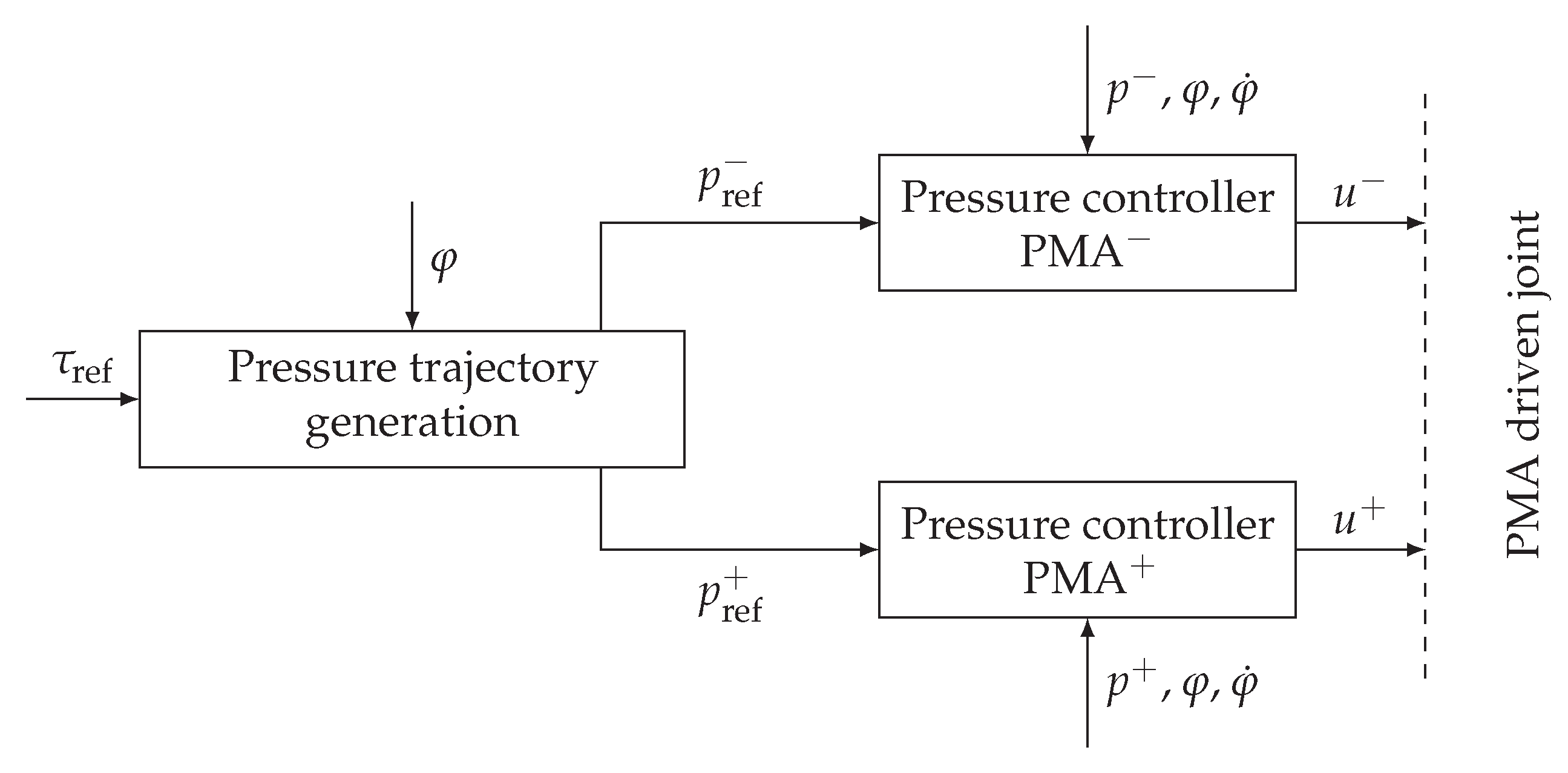
2.2.2. Pressure Trajectory Generation by Mean Pressure Definition—”PM-Approach”

Since the PMA force was accurately defined in the previous section, we now present a first approach for solving (2) with respect to the pressures p ± . By connecting both PMA pressures by the constraint of a common mean pressure
p m = p + + p 2 ,
the system of equations becomes solvable, such that p ± can be calculated from a given torque trajectory. Therefore, this torque control approach will be denoted as the PM-approach. Postulating the mean pressure is known, the Equations (2) and (10) can be solved for pressures p + and p . For example, p is found to be
p = τ R + 2 p m A ( L + ) + B ( L ) B ( L + ) A ( L + ) + A ( L ) .
According to the PMA data sheet [31], their maximum contraction is about 25%. Taking a closer look to (11), it is clear that A ( L + ) + A ( L ) 0 has to be guaranteed for all L ± 0.75 L 0 , L 0 , because singularities would occur otherwise. Theorem A2 guaranties that A ( L + ) + A ( L ) 0 as long as L 0.7 L 0 , L 0 and θ 0 0 ° , 34.4332 ° . The theorem itself and its proof can be found in Appendix A. For the sake of safety, and just in case the PMA contraction is not in accurate accordance with the data sheet, in this paper, the maximum contraction is supposed to be 30 %.
By inserting (11) back into (10) the second pressure
p + = 2 p m p
can easily be calculated.
The mean pressure, supposed to be known but not set to a specific value so far, can be used to fulfill additional constraints. Because PMAs are only pulling actors and pulling forces are defined to be positive for this paper, a very important constraint is that both PMA forces stay positive ( F ± 0 ) at any time. This constraint guarantees tight ropes and, therefore, no loss of contact between the PMAs and the pulley. Figure 3 shows the characteristics of the mean pressure p m for the given constraint F ± 0 .
A consequence of connecting two PMAs, each of which can exert a force, to one pulley, is that the force map of the first PMA overlays the force map of the second. As already noted, both PMAs are connected at half contraction and this is defined as φ = 0 . If both PMAs are equivalent, their connection at half contraction leads to a symmetric angle range, i.e., φ min = φ max . The force map of one PMA is a function of the PMA internal pressure and its length. The PMA lengths cannot be chosen independently and are defined by the angular position of the pulley. Therefore, Figure 3a shows the PMA force above the PMA pressure and the angular position of the pulley. Figure 3b is a top view of Figure 3a. The angle range [ φ min , φ max ] is dependent on the initial PMA length and the chosen pulley radius. The pressure range [ p 0 , p s ] is between the atmospheric pressure p 0 and the chosen supply pressure p s .
The colors black and blue in Figure 3 are related to F + and F , respectively. According to this, the blue and black curved diagonals representing the zero-force lines of the force map of PMA + p 0 F + (black) and PMA p 0 F (blue) respectively. The area of F + 0 is therefore the upper left, the area of F 0 the upper right, curved triangle.
At this point the question is how the mean pressure p m has to be defined in advance, to make sure that no rope is hanging loose. This can be guaranteed by determining the common mean pressure in the following way, and only by using an overlay of two static PMA force maps (Figure 3):
  • For every angle the upper individual mean pressure— p m (blue dashed) respectively p m + (black dashed)—is set to be in the middle of p 0 F ± and the supply pressure p s .
  • The lower individual mean pressure is calculated such that the forces of both PMAs are equal, if both PMAs are filled with their individual mean pressure.
  • For any time the pressure p + has to be inside the black, the pressure p inside the blue area. The pressures are limited by the supply pressure and the pressure of zero force p 0 F , because otherwise the rope would hang loose. Furthermore, both pressures are always equidistant to the mean pressure p m and the smaller force range, defined by the pressure range around the individual mean pressures limits both pressure ranges.
  • The common mean pressure p m (bold black line) is a result of (10).
The torque characteristics of this pressure trajectory calculation can be seen in Figure 4. For any application it is important to say that, as long as the torque stays within the range depicted in Figure 4, the PMA forces will—with the calculated mean pressure p m —always be greater than zero and the ropes will be tight.

2.2.3. Pressure Trajectory Generation by Force Separation—“FIT-Approach”

As first presented in [26], separating the torque in two forces and defining that each PMA is only responsible for a torque in one direction, the forces are given through
F + = | τ | R + F IT if τ 0 F IT if τ < 0 F IT 0 and
F = F IT if τ 0 | τ | R + F IT if τ < 0 . F IT 0
The force F IT can be interpreted as an initial tension. Therefore, this torque control approach will be called the FIT-approach. The pressures p ± can be easily calculated by inserting the PMA length and its force in (4), which yields
p ± = B ( L ± ) F ± A ( L ± ) .
An advantage of this approach is that it implicitly fulfills the important constraint F ± 0 , without any further calculations. Theorem A1 guarantees that A ( L ) 0 as long as L 0.7 L 0 , L 0 and θ 0 0 ° , 34.4332 ° . The theorem itself and its proof can be found in Appendix A.

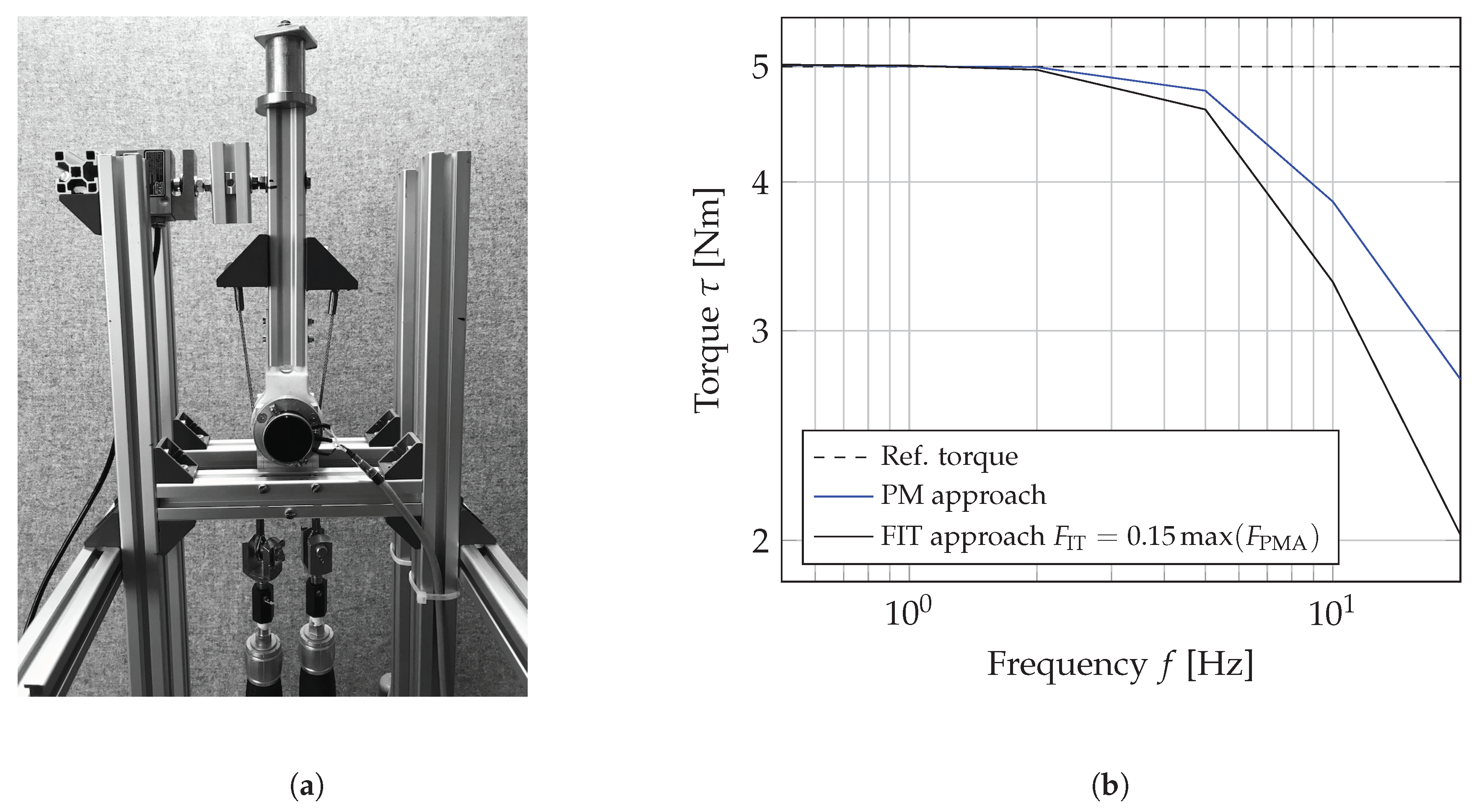
2.2.4. A Comparison of Two Torque Characteristics

In Section 2.2.2 and Section 2.2.3 two different ways are shown, how one torque trajectory can be translated into two pressure trajectories. In Figure 4, the resulting torque ranges, also denoted as the torque characteristics are depicted.
While the approach of force separation has the ability to exploit the whole work potential of both PMAs, the mean pressure approach seems to use most of the PMA forces as initial tension, such that only a small amount of force can be used to generate a torque. Especially at the edges of Figure 4a, it stands out that no torque can be exerted anymore with the approach of a common mean pressure. Furthermore, it is interesting to see that the maximum torque at the edges with the approach of force separation can only be exerted in one direction. However, the maximum torque can only be exerted if the force F IT equals zero. In case of F IT > 0 (see Figure 4b), the maximum torque as well as the angle range are decreasing [26].

2.3. Bandwidth of the Torque Controller

As depicted in Figure 2, the torque controller consists of a pure algebraic pressure trajectory generation and two pressure controllers with a given bandwidth. Accordingly the torque controller must have the same bandwidth as the pressure controllers, i.e., the torque controller design boils down to a design of two similar pressure controllers for each PMA. A decoupling servo pressure controller for PMAs is presented in [32], and will be employed in the current publication as well.

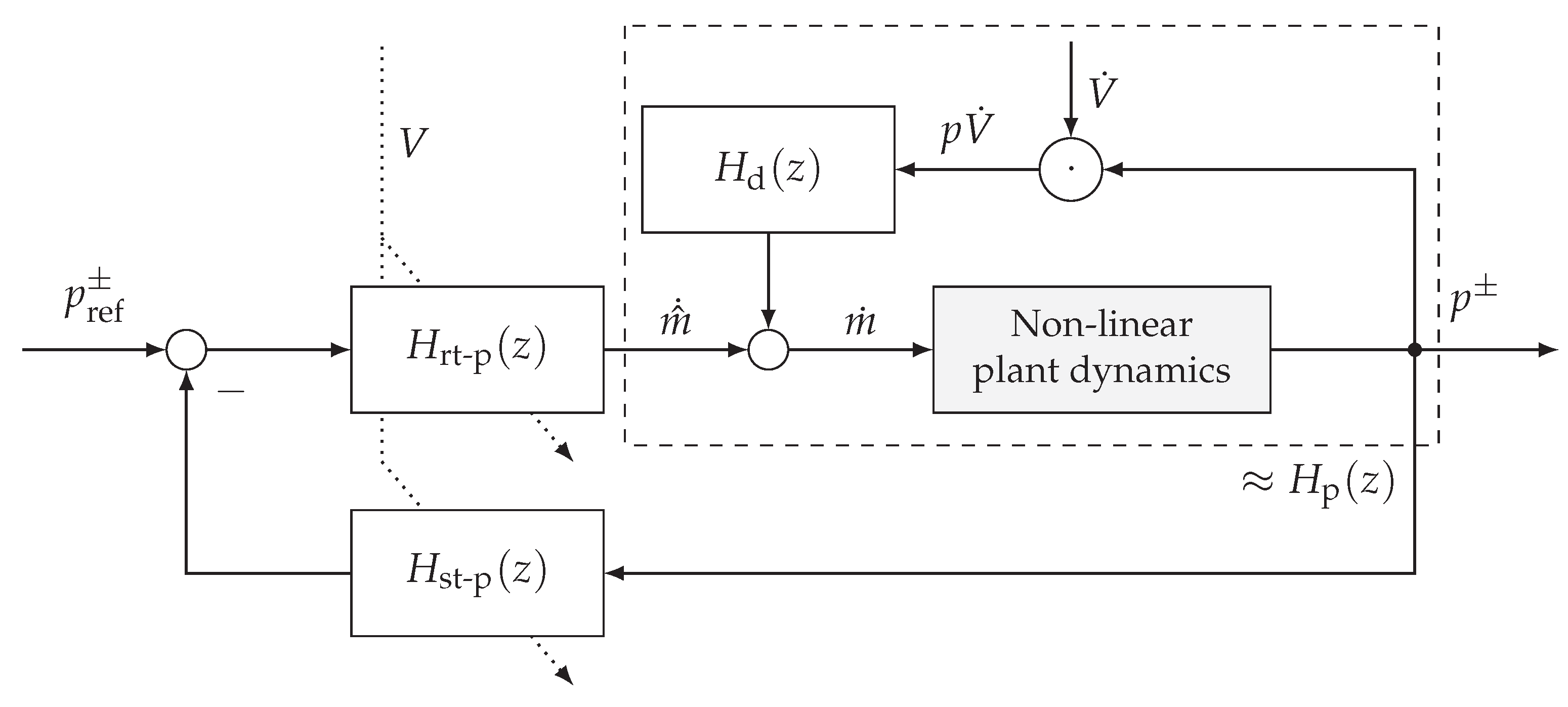
2.3.1. Pressure Dynamics

The pressure dynamics of the PMA consists of three different parts: At first, the air inside the PMA has its own fluid dynamics. Furthermore, the mass flow shaped by the pneumatic valve and the valve dynamics must be included in the model. The PMA pressure dynamics
p ˙ = χ R T V m ˙ χ p V ˙ V
can be found e.g., in [32], where χ is the polytropic coefficient and R ( 288 Nm/kgK under reference conditions) is called the ideal gas constant. In [14] the polytropic exponent was identified by measurement as χ = 1.26 for PMAs, i.e., state changes of the included air are somewhere in between isothermal ( χ = 1 ) and isentropic ( χ = 1.4 ) conditions.
Furthermore, the mass flow
m ˙ = C ( x ) p s ρ 0 T 0 T 0 p p s < b x 0 , 1 C ( x ) p s ρ 0 T 0 T 1 p p s b 1 b 2 b p p s 1 x 0 , 1 C ( x ) p ρ 0 T 0 T 1 p 0 p b 1 b 2 b p 0 p 1 x 1 , 0 C ( x ) p ρ 0 T 0 T 0 p 0 p < b x 1 , 0
passing through a pneumatic valve can be calculated according to ISO 6358 or [33]. In this equation, p 0 = 100 kPa and T 0 = 293.15 K represent the pressure and the temperature under reference conditions, respectively. Furthermore, (17) can be read in the following way: dependent on the valve slide stroke x and the pressure ratio p / p s , respectively, p 0 / p , the mass flow is divided in four different cases. For x [ 0 , 1 ] —i.e., inflation, the supply pressure p s is connected to the PMA volume. For x [ 1 , 0 ) , i.e., deflation, the PMA volume is connected to atmospheric pressure. Furthermore, the fluid flows with the local speed of sound in at least one section of the valve for 0 p / p s < b , respectively, 0 p 0 / p < b (choked flow) or with subsonic speed for b p / p s 1 , respectively, b p 0 / p 1 (subsonic flow).
The general form of (17) is adapted to a specific form by inserting a specific critical pressure ratio b and sonic conductance C, which characterize a particular valve. For the present paper this will be a Festo MPYE-5-1/8-LF-010-B proportional servo valve. The critical pressure ratio of this valve can be treated as constant and is identified by measurement to b = 0.35 . The sonic conductance C has been measured in dependency of the normalized valve slide stroke. The measured values are depicted in Figure 5 and can be found in Appendix C.
The slide stroke of the Festo MPYE-5-1/8-LF-010-B is controlled by an internal position controller. According to [34,35] the transfer function, which relates the normalized valve control signal u [ 1 , 1 ] and the normalized valve slide stroke x [ 1 , 1 ] , can be approximated by a first-order lag filter. The transfer function is given in the frequency domain, whereby X and U are the Laplace transform of the control signal and the valve slide stroke, respectively:
X ( s ) U ( s ) = 1 T v s + 1 .
The time constant T v = ω v 1 = ( 2 π f v ) 1 can be calculated from the valve cut-off frequency f v = 95 Hz [34] provided in the data sheet of the Festo MPYE-5-1/8-LF-010-B proportional servo valve.

2.3.2. Controller Design

In [32], a pressure controller for PMAs is presented and tested. Furthermore, it is shown that a linear controller design becomes feasible if the pressure changes, which are related to time-varying volume, are treated as observable disturbance, which can be easily compensated. In contrast to the controller design of [32], the first-order lag (18) is neglected in the current contribution. Therefore, the input signal u equals the valve-slide stroke x.

Mass Flow as Virtual Input

In accordance to [32], the mass flow can be treated as a new, virtual input signal if (17) is inverted:
C = m ˙ ρ 0 p s T T 0 0 p < b p s m ˙ 0 m ˙ ρ 0 p s T T 0 1 p p s b 1 b 2 1 2 b p s p p s p ε m ˙ 0 m ˙ ρ 0 p T T 0 1 p 0 p b 1 b 2 1 2 p 0 + p ε p p 0 b m ˙ < 0 m ˙ ρ 0 p T T 0 p 0 b < p m ˙ < 0 .
To avoid singularities the pressure is limited to p 0 + p ε and p s p ε , where the pressure gap is set to p ε = 0.1 Pa.
Since the sonic conductance C ( x ) , as depicted in Figure 5, is a monotonically increasing function of x, numerical inversion is straight forward, and the dependency x ( C ) = u ( C ) can be calculated easily.

Interpreting the Plant as a Linear Time-Invariant System

The latter summand χ V p V ˙ in (16) can be interpreted as a disturbance. By choosing the mass flow
m ˙ = m ^ ˙ + 1 R T = : G d ( s ) · p V ˙ ,
the disturbance can be compensated and m ^ ˙ becomes the new input mass flow. By choosing the mass flow like this, each PMA is being decoupled pneumatically from every other PMA driving the system, such that a separated and local pressure control design for each PMA is facilitated.
Through approximating the volume inside the PMA by a constant volume V = V ¯ and setting the temperature to the constant ambient temperature T = T a = T 0 , the new plant dynamics G p is described by the linear time-invariant system
G p ( s ) = p m ^ ˙ = χ R T a V ¯ 1 s .

2.3.3. Pressure Controller Design

The continuous plant dynamics (21) is sampled with a sampling frequency of T s 1 = f s = 1 kHz, i.e., the sampling frequency is about one decade higher than the highest plant frequency of 95 Hz, defined by the pneumatic servo valve. Using a zero-order hold discretization, the z-transform of the plant is given by
H p ( z ) = χ R T a V ¯ T s ( z 1 )
which has only an integrating pole at z = 1 . Following the polynomial controller design procedure explained in [36], a so called RST digital pressure controller can be designed for pressure regulation inside a constant volume. It must be noted that the notation is in accordance with the notation of [36], i.e., the controller polynomials are denoted by S p ( z ) , T p ( z ) and R p ( z ) , and the controller consists of two discrete-time transfer functions H rt p ( z ) = T p ( z ) / R p ( z ) and H st p ( z ) = S p ( z ) / T p ( z ) , respectively.
Although it is shown in [32] that one single controller, designed e.g., for the initial PMA volume V 0 , is able to control the PMA pressure with satisfying results, in this paper an adaptive gain-scheduling controller will be used for pressure regulation, because this approach improves the performance of the pressure controller. Therefore, multiple RST-controllers are designed for ten different volume values within V ¯ [ V ( L 0 ) , V ( 0.7 L 0 ) ] , and their coefficients are interpolated linearly in real time. Furthermore, the controller is extended by a disturbance cancellation H d ( z ) , which is the z-transform of G d ( s ) from (20), as proposed in [32]. The whole control structure is schematically depicted in Figure 6. In order to determine the time-derivative of the volume V ˙ without amplification of measurement noise, an algebraic derivative estimation algorithm presented in [37,38] is applied to the calculated PMA volume (7).
In the present paper, the controller is designed as a servo controller that can be used e.g., as the inner controller of a cascade-structured controller. In case integral action is required or the controller has to fulfill some other requirements like frequency suppression, this can be done very easily by defining the zeros of R p ( z ) and S p ( z ) [36].
According to the degree condition given in [36], the degree of the closed loop polynomial d e g ( A cl p ( z ) ) increases with any additional zero of R p ( z ) and S p ( z ) . As a consequence of the chosen two-degrees-of-freedom control structure, the closed loop poles can be further subdivided into so called observer poles and so called controller poles and only the latter ones are defining the visible dynamics of the closed control loop. The amount of the controller poles equals the number of plant poles, such that the controller has only one controller pole and the remaining deg ( A cl ) 1 poles are all observer poles. The closed loop polynomial
A cl p ( z ) = ( z P c ) · i = 1 deg ( A cl ) 1 z P o , i
shows that, independent of the number of observer poles, the two degrees of freedom control structure enables their cancellation, such that only the controller pole
P c = e 2 π T s f bw
defines the bandwidth f bw of the closed control loop. Therefore,
H cl p = 1 P c z P c
represents the transfer function of the closed pressure control loop. As already noted, the torque controller must have the same bandwidth such that also the torque control loop can be described by
H cl τ = 1 P c z P c .

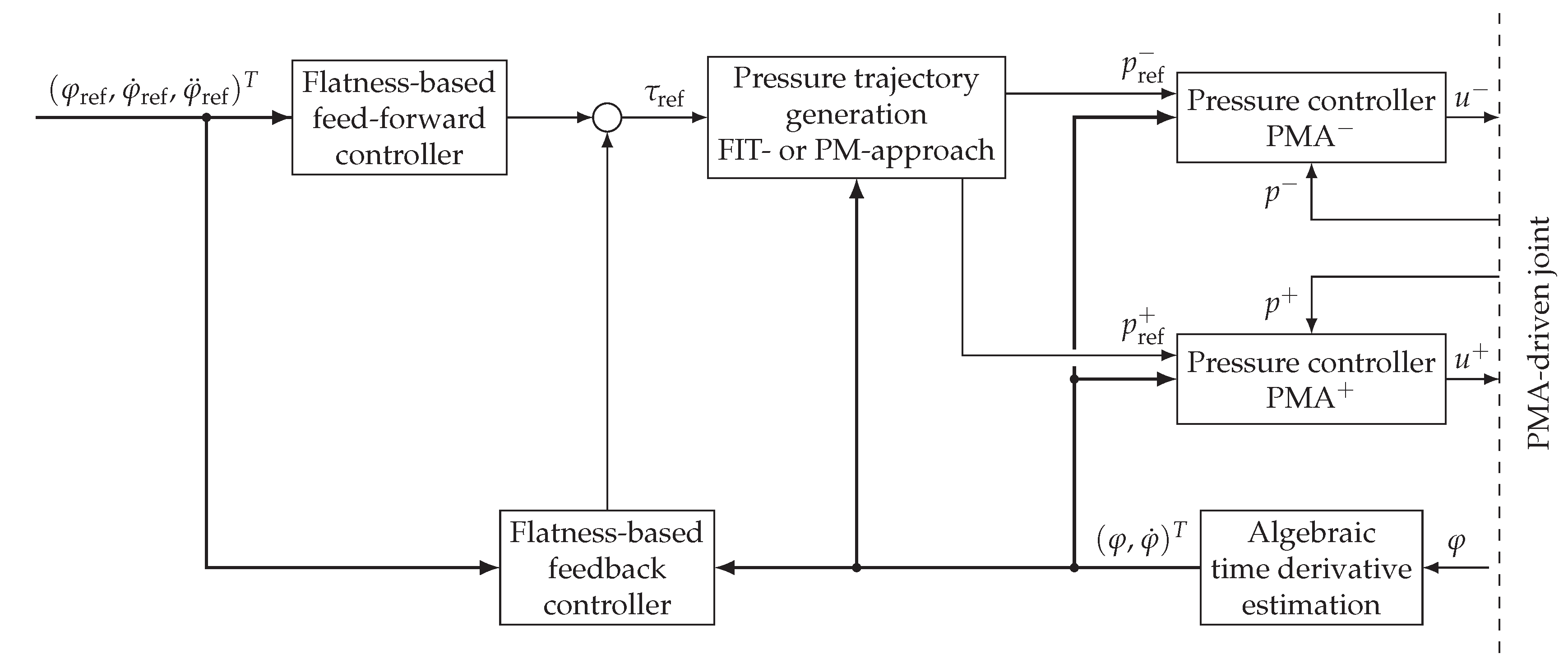
3. Angular Position Controller for an Exemplary Robotic Arm

In this section, an angular position controller for an exemplary robot with one degree of freedom, as depicted in Figure 7, will be designed. Therefore, both of the torque controllers presented in the previous section are used as inner controllers for the cascade-structured motion controller. Although the robot is driven by PMAs, it will be shown that the motion controller design becomes simplified by pre-controlling the torque of the PMA-driven joint, because only its bandwidth and torque characteristics have to be taken into account for an overlying controller design.
The target control platform is a MicroDAQ E2000 (Embedded Solutions, ul. Rzeszowska 74b, 39-100 Ropczyce, Poland), which can be programmed via a MATLAB (R2015b, The MathWorks, Inc., Natick, MA, USA) Simulink toolbox.

3.1. Inner Torque Control Loop

As depicted in Figure 2, the torque controller consists of two similar pressure controllers and an algebraic pressure trajectory generation from (11) and (12) or (13) and (14). The torque control bandwidth, represented by the controller pole P c in (25), is set to 20 Hz, i.e., the closed-loop dynamics of the torque control, sampled with a frequency of 1 kHz, is represented by
H cl τ = 1 0.8819 z 0.8819 .
While all observer poles are set to ≥ 40 Hz, the further pressure controller design is carried out by canceling the influence of measurement noise. Beside signals at the Nyquist frequency, also signals with frequencies of 101.5 Hz, 203.67 Hz, 272 Hz, 305.67 Hz and 408 Hz get suppressed by the controller, because frequency folding occurs otherwise. Furthermore, the controller design is repeated for ten different volumes, which are chosen equidistantly within V ¯ [ V ( L 0 ) , V ( 0.7 L 0 ) ] .
The robot arm, depicted in Figure 7, is actuated by two Festo DMSP-20-300. The pulley radius of R = 23.24 mm and a supply pressure of p s = 6 bar are resulting in a maximum joint torque of 35.92 Nm with the approach of force separation ( F IT = 0 ) at the edges and 14.7 Nm with the approach of a common mean pressure in the middle of the angle range, respectively (see Figure 4a). The valid angle range is limited to φ [ 97.15 ° , 97.15 ° ] . During the experiments, it turned out that the system stiffness of the PMA-driven joint is almost equivalent for both torque control approaches for an initial force of F IT = 0.15 max ( F PMA ) . Due to this, the “FIT-approach” was used with this initial force during all experiments. Like as it can be seen in Figure 4b, the angle range as well as the maximum torque are decreasing through increasing the initial tension while using the “FIT-approach”. The maximum torque of the “FIT-approach” controller with an initial tension F IT = 0.15 max ( F PMA ) is τ max = 19.4284 Nm. The valid angle range is reduced to φ [ 58.19 ° , 58.19 ° ] .
To proof the functionality of the torque controller, the robot arm was fixed in an upright position and screwed to a force sensor KD40 s ± 2 kN (ME-Meßsysteme GmbH, Neuendorfstr. 18a, DE-16761 Hennigsdorf, Germany). The measured force signal is amplified by a GSV-1A measurement amplifier (ME-Meßsysteme GmbH, Neuendorfstr. 18a, DE-16761 Hennigsdorf, Germany) and multiplied with a lever arm of 200 mm such that the exerted torque of the PMA-driven joint in this position becomes measurable. This position represents the center of the angle range, i.e., φ = 0 , and both PMAs are at their mean length of 260.6 mm. The whole measurement setup can be seen in Figure 8a.
During measurements, the PMA-driven joint was following a sine torque trajectory with an amplitude of 5 Nm and frequencies of 0.5 Hz, 1 Hz, 2 Hz, 5 Hz, 10 Hz and 20 Hz. All amplitudes of the exerted torque as well as the reference of 5 Nm are depicted in Figure 8a,b. The black line shows the measured torque amplitude of a “FIT-approach” torque controller with an initial force of 15% of the maximum PMA force and the blue line shows the torque amplitude of a “PM-approach” torque controller. While both control approaches have a cut-off frequency of about 10 Hz, it can be seen that the cutoff frequency of the “PM-approach” controller is slightly higher. A reason for this can be found in the way the pressure trajectories are generated. Depending on whether the torque is positive or negative, the “FIT-approach” controller only varies one pressure, while the other one is kept constant. In contrast to this, the “PM-approach” controller always varies both pressures at the same time for exerting a given torque trajectory.

3.2. Outer Angular Position Controller

The equation of motion of the 1-DOF robotic arm, depicted in Figure 7, in an upright position is given by
φ ¨ = ω 0 2 m g l s τ 2 δ m g l s ω 0 2 φ ˙ m g l s sin φ .
The parameters ω 0 and δ were determined to ω 0 = 6.1995 s 1 and δ = 0.025439 s 1 , respectively, by analyzing the oscillation of the robotic arm around the stable equilibrium in the hanging position. Furthermore, the arm mass with additional load mass is m = 1.672 kg and the distance from the center of rotation to the arm center of mass is l s = 246.1 mm. The acceleration is about 9.81 ms 2 .
By defining the system output as y = φ , all state variables
φ = y
φ ˙ = y ˙
as well as the input
τ = m g l s ω 0 2 y ¨ + 2 δ y ˙ ω 0 2 sin y
are defined only by the chosen output and its time derivatives. Likewise it can be said that the system is differentially flat and the output φ can be denoted as one flat output of the system [39].
Due to the flat system characteristic, the control torque
τ ref = m g l s ω 0 2 φ ¨ ref + 2 δ φ ˙ ref ω 0 2 sin φ ref + f ( e , e ˙ ) e = φ φ ref
can be further subdivided into a feed-forward controller—represented by the inverted equation of motion—and feedback controller that stabilizes the system. The control structure can be found in Figure 9.
The controller (32) defines an error dynamics of the controlled system
e ¨ + 2 δ e ˙ ω 0 2 cos φ ref e f ( e , e ˙ ) = 0 ,
which can be stabilized by
f ( e , e ˙ ) = ω 0 2 cos φ ref e K p e K d e ˙ K i e d t .
By transforming the resulting error dynamics to the frequency domain, the poles of the characteristic polynomial
s 3 + ( 2 δ + K d ) s 2 + K p s + K i = 0
can be placed arbitrarily through a variation of the controller gains K p , K i and K d . For this paper the characteristic equation is separated in one conjugate-complex pole pair that dominates the error dynamics and a third pole on the real axis. For the sake of stability, the real part of all three poles is kept strictly negative. Stability as well as further requirements can be specified by defining a desired error dynamics
( s 2 + 2 δ 12 s + ω 12 2 ) ( s + ω 3 ) = 0 ,
to which the original error dynamics (35) can be transformed by comparing the coefficients of (35) and (36). The resulting controller gains are
K d = 2 δ 12 + ω 3 2 δ K p = ω 12 2 + 2 δ 12 ω 3 K i = ω 12 2 ω 3 .
Through iterative, hardware-in-the-loop testing the parameters of the desired error dynamics where finally set to ω 12 = 15.625 s−1, δ 12 = 10 s−1 and ω 3 = 15.625 s−1.

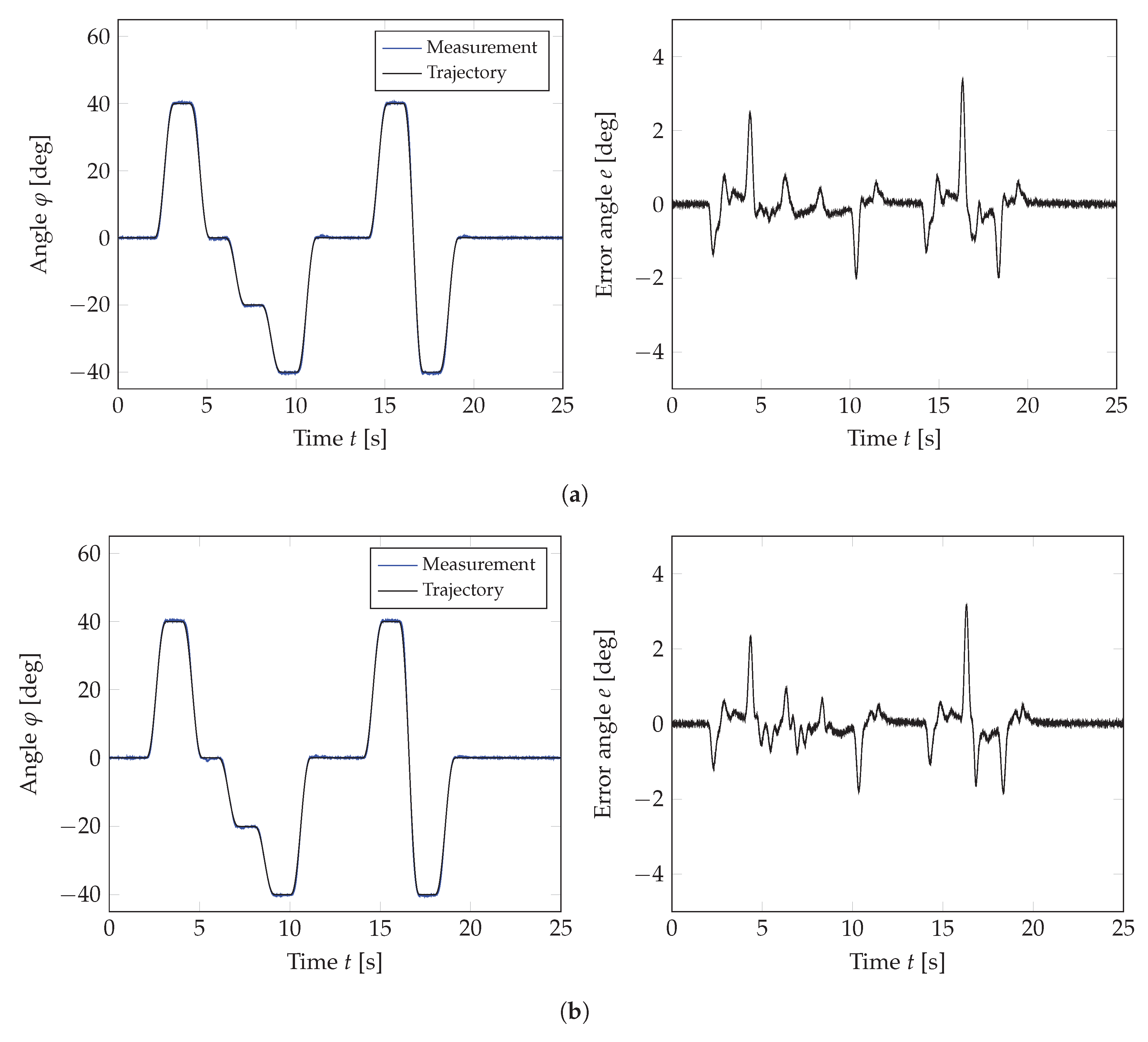
3.3. Experimental Investigation of the Trajectory Following Behavior

The presented cascade-structured angle controller is tested by experimental investigation of its ability to follow a given angle trajectory. The chosen flatness-based controller always needs, in addition to the reference angle, also its first and second time derivative. Therefore, the reference trajectory is calculated such that it guarantees a continuous time evolution of the angle, the angular velocity and the angular acceleration. Figure 10 shows the defined reference angle trajectory and the tracking behavior of the presented angle controllers. While Figure 10a shows the angle tracking behavior with the underlying “PM-approach” torque controller, Figure 10b shows the angle tracking performance with the same flatness-based angle controller, but with the underlying “FIT-approach” torque controller. The initial force of this approach is set to F IT = 0.15 max ( F PMA ) , because this initial force leads to almost equivalent system stiffness as the “PM-approach”.
On the left hand side of Figure 10, it can be seen that the trajectory as well as the system angle are almost identical and this is the same for both torque control approaches. The error, defined as e = φ φ ref , is almost the same for both torque control approaches and only minor differences can be noticed. While the maximum error angle is about 3 ° the error seems a little rougher for the “FIT-approach” than for the “PM-approach”. In other words: the “PM-approach” reacts a little bit faster such that control errors can be counteracted a little better in comparison to the “FIT-approach”. This correlates with the slightly higher bandwidth of the “PM-approach” torque controller (see Figure 8). Nevertheless, both torque control approaches lead to excellent results and both are representing a very useful interface controller for an overlying motion controller, like e.g., the presented flatness-based controller. But also any other motion controller can be easily interconnected to a robot with PMA-driven joints via one of the presented torque controllers. Furthermore, the presented control framework is not limited to a one-degree-of-freedom robot but is suitable for any robot with multiple degrees of freedom.

4. Conclusions

In this paper, a new control framework for robots driven by PMA-driven joints was presented and successfully applied to a robot with one degree of freedom. This framework connects PMA-driven joints and their challenging characteristics, on the one hand, and “classic” robotic control methods, on the other hand. By using a torque controlle—one for every PMA-driven joint—as an interface, the design of an overlaying motion controller becomes simplified, even for robots with multiple degrees of freedom. Furthermore, once the PMA-driven joint is torque-controlled, all difficulties of controlling a PMA-driven joint get handled internally, i.e., the PMA-driven joint can be treated as pure torque source with a given bandwidth. The maximum torque amplitude that the PMA-driven joint can exert is limited by a static torque characteristic that is defined by the chosen torque control approach.
At the beginning of this paper, two variants of a torque controller were developed. The first torque control approac—“PM-approach”—defines a common mean pressure for both PMAs that are driving one joint, i.e., only the symmetric pressure difference around the mean pressure defines the torque the PMA-driven joint exerts. In contrast to this, the second approach—“FIT-approach”—directly separates the forces for each PMA, i.e., the PMA force equation can be solved for both PMA pressures separately. Although it is shown that the cut-off frequency of both approaches is almost the same (about 10 Hz for a PMA-driven joint with two Festo DMSP-20-300 for this pape), it can be seen that the “PM-approach” is slightly faster. The reason is that the “PM-approach” varies both PMA pressures, i.e., one PMA works in collaboration with the other PMA to exert a desired torque. In contrast to this, the “FIT-approach” uses only one PMA to exert a positive torque and the other one a torque in the opposite direction. An advantage of this approach is its ability to use the full work potential of each PMA, while the “PM-approach” uses most of the PMA force as initial tension. In summary it can be said that the “PM-approach” is slightly faster than the “FIT-approach” torque controller, but the maximum torque can be higher with the second approach. However, controlling the torque of a PMA-driven joint is suitable with both approaches.
Finally, both torque controllers have been included in a flatness-based angle controller design for an exemplary robotic arm. By investigation of their trajectory following behavior, it was demonstrated that both torque control approaches can lead to high performance angle controllers with very low tracking error. However, for the presented robot and the tracking control task, the “PM-approach” leads to slightly better results, because of its higher bandwidth.
Finally, it should be noted that the presented control framework is not limited to the use of the presented one-degree-of-freedom robot. The application of this framework to multiple-degrees-of-freedom robots will probably be included in future work.

Author Contributions

M.M. developed the torque control framework for PMA-driven joints. Furthermore, M.M. designed the angle controller for the robot used for all experiments and also executed all experiments. I.B. was the main supervisor and adviser of the work, he was involved in discussion of the methods and the experimental design. T.S. was involved in discussion of the mathematical analysis and the experimental results. J.Z. crucially supported the execution of all experimental procedures.

Funding

All presented research results have been supported by the German Federal Ministry for Economic Affairs and Energy (BMWi), especially The Central Innovation Program for SMEs and the research project Development of a PMA-driven Exoskeleton for the Upper Body (project number ZF4007503).

Acknowledgments

Special thanks are extended to Amador Cabos, who measured the sonic conductance and the critical pressure ratio of the pneumatic servo valve Festo MPYE-5-1/8-LF-010-B according to the ISO 6358.

Conflicts of Interest

The authors declare no conflict of interest. The founding sponsors had no role in the design of the study; in the collection, analysis, or interpretation of data; in the writing of the manuscript, and in the decision to publish the results.

Appendix A. Proof A(L) ≠ 0 and A(L+) + A(L) ≠ 0

According to the PMA data sheet [31], their maximum contraction is about 25%. For the sake of safety, in this paper the maximum contraction is supposed to be 30%, i.e., the initial length L 0 and 0.7 L 0 are limiting the PMA length range. It is of interest to know if A ( L ) , defined in (4) becomes zero within this length range, because this would cause singularities in (15). Where A ( L ) becomes zero is mostly defined by the initial fiber angle θ 0 . For the DMSP-20-300, used as an exemplary PMA in this paper, the initial fiber angle is identified as θ 0 ( D M S P 20 300 ) = 25.9952 ° . The factor n in (5) represents the number of windings of the fibers inside the PMA membrane (see [25] for more information) and according to (6) it stays strictly positive for 0 ° < θ 0 < 90 ° .
Theorem A1.
Let L represent the length of a Festo PMA and θ 0 its initial fiber angle. If θ 0 0 ° , 34.4332 ° then A ( L ) = L Fiber 2 3 L 2 / 4 π n 2 0 L 0.7 L 0 , L 0 .
Proof. 
Let L [ 0.7 L 0 , L 0 ] , θ 0 0 ° , 34.4332 ° and A ( L ) = 0 . It follows that
A ( L ) = L Fiber 2 3 L 2 4 π n 2 = 0 4 π n 2 > 0 L Fiber 2 3 L 2 = 0 L Fiber 2 = 3 L 2 L 0 2 3 ( cos θ 0 ) 2 = L 2 L > 0 L = L 0 2 3 ( cos θ 0 ) 2 = 1 3 cos θ 0 0.5774 , 0.7 · L 0 [ 0.7 L 0 , L 0 ]
According to this, A ( L ) 0 L [ 0.7 L 0 , L 0 ] holds true for all Festo PMAs with θ 0 0 ° , 34.4332 ° . □
Furthermore, it is important to know if A ( L + ) + A ( L ) becomes zero for any L [ 0.7 L 0 , L 0 ] , because this would cause singularities in (11) and (12), respectively.
Theorem A2.
Let L ± [ 0.7 L 0 , L 0 ] represent the lengths of two PMAs of a PMA-driven joint and let θ 0 be their initial fiber angle. If A ( L ± ) 0 θ 0 0 ° , 34.4332 ° then A ( L + ) + A ( L ) 0 θ 0 0 ° , 34.4332 ° .
Proof. 
According to Theorem A1, A ( L ) does not change the leading sign for L [ 0.7 L 0 , L 0 ] and θ 0 0 ° , 34.4332 ° . Furthermore, as a combination of continuous functions, A ( L ) is a continuous function. This implies that A ( L + ) + A ( L ) must have the same sign, such that
A ( L + ) + A ( L ) = 0 A ( L + ) = 0 A ( L ) = 0 .
It follows that A ( L + ) + A ( L ) 0 L ± [ 0.7 L 0 , L 0 ] holds true for all Festo PMAs with θ 0 0 ° , 34.4332 ° . □

Appendix B. Force Map Festo DMSP-20-300

Force [N]
Length [mm]224226227229231232234235238240243245250253260264276278289290296297299
Rel. Pressure [Pa]
10,00000000000000000000000029
50,0000000000000000000000−3119196
100,0000000000000000000−7013101125209216
150,00000000000000000008312123212245331343
200,000000000000000106912176112236325370456471
250,000000000000000601214191270212353440495580599
300,0000000000010471211976214170365313470556622706729
350,0000000002043129667178140287249460413588671748831857
400,00000001040108658145121237204360329555513705787874955986
450,000000035107852129105193174295268433409649613822902100010801115
500,000001.5227047116931711512422283543325054887447139391018112512041243
550,0000621.554.51058415413421419829128141339657856683881310561132125013281371
590,0000284680.513211418416624823532932446044763662991389211491224134814271472

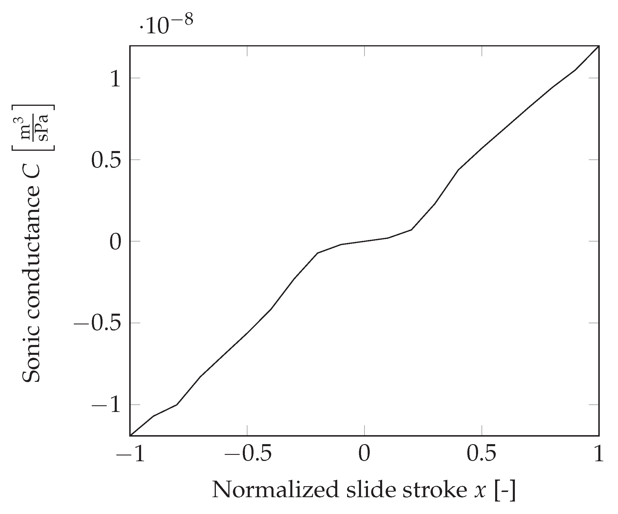
Appendix C. Sonic Conductance Festo MPYE-5-1/8-LF-010-B

xC(x) · 10 8 xC(x) · 10 8 xC(x) · 10 8
1 1.19 0.3 0.23 0.4 0.44
0.9 1.07 0.2 0.07 0.5 0.57
0.8 1.00 0.1 0.02 0.6 0.69
0.7 0.83 0 0.00 0.7 0.82
0.6 0.70 0.1 0.02 0.8 0.94
0.5 0.56 0.2 0.07 0.9 1.05
0.4 0.42 0.3 0.23 1 1.20

References

  1. Andrikopoulos, G.; Nikolakopoulos, G.; Manesis, S. A survey on applications of pneumatic artificial muscles. In Proceedings of the 2011 19th Mediterranean Conference on Control & Automation (MED), Corfu, Greece, 20–23 June 2011; pp. 1439–1446. [Google Scholar]
  2. Caldwell, D.G.; Tsagarakis, N.G.; Kousidou, S.; Costa, N.; Sarakoglou, I. “Soft” exoskeletons for upper and lower body rehabilitation—Design, control and testing. Int. J. Humanoid Robot. 2007, 4, 549–573. [Google Scholar] [CrossRef]
  3. Cao, J.; Xie, S.Q.; Das, R. MIMO sliding mode controller for gait exoskeleton driven by pneumatic muscles. IEEE Trans. Control Syst. Technol. 2018, 26, 274–281. [Google Scholar] [CrossRef]
  4. Noritsugu, T.; Tanaka, T. Application of rubber artificial muscle manipulator as a rehabilitation robot. IEEE/ASME Trans. Mechatron. 1997, 2, 259–267. [Google Scholar] [CrossRef] [Green Version]
  5. Hošovskỳ, A.; Pitel’, J.; Židek, K.; Tóthová, M.; Sárosi, J.; Cveticanin, L. Dynamic characterization and simulation of two-link soft robot arm with pneumatic muscles. Mech. Mach. Theory 2016, 103, 98–116. [Google Scholar] [CrossRef]
  6. Schindele, D.; Aschemann, H. Trajectory tracking of a pneumatically driven parallel robot using higher-order SMC. In Proceedings of the 2010 15th International Conference on Methods and Models in Automation and Robotics (MMAR), Miedzyzdroje, Poland, 23–26 August 2010; pp. 387–392. [Google Scholar]
  7. Schindele, D.; Aschemann, H. P-type ILC with phase lead compensation for a pneumatically driven parallel robot. In Proceedings of the 2012 American Control Conference (ACC), Montreal, QC, Canada, 27–29 June 2012; pp. 5484–5489. [Google Scholar]
  8. Andrikopoulos, G.; Nikolakopoulos, G. HUmanoid Robotic Leg via pneumatic muscle actuators: Implementation and control. Meccanica 2018, 53, 465–480. [Google Scholar] [CrossRef]
  9. Dirven, S.; McDaid, A. A Systematic Design Strategy for Antagonistic Joints Actuated by Artificial Muscles. IEEE/ASME Trans. Mechatron. 2017, 22, 2524–2531. [Google Scholar] [CrossRef]
  10. Siciliano, B.; Sciavicco, L. Robotics—Modelling, Planning and Control; Springer: London, UK, 2012. [Google Scholar]
  11. Lynch, K.M.; Park, F.C. Modern Robotics: Mechanics, Planning, and Control; Cambridge University Press: Cambridge, UK, 2017. [Google Scholar]
  12. Boblan, I.; Maschuw, J.; Engelhardt, D.; Schulz, A.; Schwenk, H.; Bannasch, R.; Rechenberg, I. A human-like robot hand and arm with fluidic muscles: Modelling of a muscle driven joint with an antagonistic setup. In Proceedings of the 3rd International Symposium on Adaptive Motion in Animals and Machines, Ilmenau, Germany, 25–30 September 2005. [Google Scholar]
  13. Shen, X. Nonlinear model-based control of pneumatic artificial muscle servo systems. Control Eng. Pract. 2010, 18, 311–317. [Google Scholar] [CrossRef]
  14. Hildebrandt, A.; Sawodny, O.; Neumann, R.; Hartmann, A. Cascaded control concept of a robot with two degrees of freedom driven by four artificial pneumatic muscle actuators. In Proceedings of the 2005 American Control Conference, Portland, OR, USA, 8–10 June 2005; Volume 1, pp. 680–685. [Google Scholar] [CrossRef]
  15. Vitiello, N.; Lenzi, T.; De Rossi, S.M.M.; Roccella, S.; Carrozza, M.C. A sensorless torque control for Antagonistic Driven Compliant Joints. Mechatronics 2010, 20, 355–367. [Google Scholar] [CrossRef]
  16. Lin, C.J.; Lin, C.R.; Yu, S.K.; Chen, C.T. Hysteresis modeling and tracking control for a dual pneumatic artificial muscle system using Prandtl–Ishlinskii model. Mechatronics 2015, 28, 35–45. [Google Scholar] [CrossRef]
  17. Aschemann, H.; Schindele, D. Comparison of Model-Based Approaches to the Compensation of Hysteresis in the Force Characteristic of Pneumatic Muscles. IEEE Trans. Ind. Electron. 2014, 61, 3620–3629. [Google Scholar] [CrossRef]
  18. Andrikopoulos, G.; Nikolakopoulos, G.; Manesis, S. Incorporation of thermal expansion in static force modeling of Pneumatic Artificial Muscles. In Proceedings of the 2015 23rd Mediterranean Conference on Control and Automation (MED), Torremolinos, Spain, 16–19 June 2015; pp. 414–420. [Google Scholar] [CrossRef]
  19. Andrikopoulos, G.; Nikolakopoulos, G.; Manesis, S. Novel Considerations on Static Force Modeling of Pneumatic Muscle Actuators. IEEE/ASME Trans. Mechatron. 2016, 21, 2647–2659. [Google Scholar] [CrossRef]
  20. Kerscher, T.; Albiez, J.; Zollner, J.; Dillmann, R. Evaluation of the dynamic model of fluidic muscles using quick-release. In Proceedings of the First IEEE/RAS-EMBS International Conference on Biomedical Robotics and Biomechatronics, 2006. BioRob 2006, Pisa, Italy, 20–22 February 2006; pp. 637–642. [Google Scholar]
  21. Schindele, D.; Aschemann, H. Model-based compensation of hysteresis in the force characteristic of pneumatic muscles. In Proceedings of the 2012 12th IEEE International Workshop on Advanced Motion Control (AMC), Sarajevo, Bosnia-Herzegovina, 25–27 March 2012; pp. 1–6. [Google Scholar]
  22. Hildebrandt, A.; Sawodny, O.; Neumann, R.; Hartmann, A. A cascaded tracking control concept for pneumatic muscle actuators. In Proceedings of the 2003 European Control Conference (ECC), Cambridge, UK, 1–4 September 2003; pp. 2517–2522. [Google Scholar]
  23. Aschemann, H.; Hofer, E.P. Nonlinear trajectory control of a high-speed linear axis driven by pneumatic muscle actuators. In Proceedings of the IECON 2006-32nd Annual Conference on IEEE Industrial Electronics, Paris, France, 6–10 November 2006; pp. 3857–3862. [Google Scholar]
  24. Schindele, D.; Aschemann, H. Nonlinear model predictive control of a high-speed linear axis driven by pneumatic muscles. In Proceedings of the American Control Conference, Seattle, WA, USA, 11–13 June 2008; pp. 3017–3022. [Google Scholar]
  25. Martens, M.; Boblan, I. Modeling the static force of a Festo pneumatic muscle actuator: A new approach and a comparison to existing models. Actuators 2017, 6, 33. [Google Scholar] [CrossRef]
  26. Martens, M.; Passon, A.; Boblan, I. A sensor-less approach of a torque controller for pneumatic muscle actuator driven joints. In Proceedings of the 2017 3rd International Conference on Control, Automation and Robotics (ICCAR), Nagoya, Japan, 24–26 April 2017; pp. 477–482. [Google Scholar] [CrossRef]
  27. Wickramatunge, K.C.; Leephakpreeda, T. Study on mechanical behaviors of pneumatic artificial muscle. Int. J. Eng. Sci. 2010, 48, 188–198. [Google Scholar] [CrossRef]
  28. Sárosi, J.; Biro, I.; Nemeth, J.; Cveticanin, L. Dynamic modeling of a pneumatic muscle actuator with two-direction motion. Mech. Mach. Theory 2015, 85, 25–34. [Google Scholar] [CrossRef]
  29. Martens, M.; Boblan, I. Erratum: Modeling the Static Force of a Festo Pneumatic Muscle Actuator: A New Approach and a Comparison to Existing Models. Actuators 2018, 7, 9. [Google Scholar] [CrossRef]
  30. Chou, C.P.; Hannaford, B. Static and dynamic characteristics of McKibben pneumatic artificial muscles. In Proceedings of the 1994 IEEE International Conference on Robotics and Automation, San Diego, CA, USA, 8–13 May 1994; Volume 1, pp. 281–286. [Google Scholar] [CrossRef]
  31. Festo, A.G. Datasheet–Fluidic Muscle DMSP/MAS. Available online: https://www.festo.com/rep/en_corp/assets/pdf/info_501_en.pdf (accessed on 27 November 2018).
  32. Martens, M.; Seel, T.; Boblan, I. A Decoupling Servo Pressure Controller for Pneumatic Muscle Actuators. In Proceedings of the 2018 23rd International Conference on Methods & Models in Automation & Robotics (MMAR), Miedzyzdroje, Poland, 27–30 August 2018; pp. 286–291. [Google Scholar]
  33. Beater, P. Pneumatic Drives; Springer: Berlin, Germany, 2007. [Google Scholar]
  34. KG, F.V.G.C. Datasheet–Proportional Directional Control Valves MPYE; Festo Vertrieb GmbH Co. KG, Festo Campus: Esslingen, Germany, 2017. [Google Scholar]
  35. Rager, D.; Neumann, R.; Murrenhoff, H. Simplified Fluid Transmission Line Model. In Proceedings of the 14th Scandinavian International Conference on Fluid Power (SICFP15), Tampere, Finland, 20–22 May 2015. [Google Scholar]
  36. Åström, K.J.; Wittenmark, B. Computer-Controlled Systems: Theory and Design, 3rd ed.; Dover Publication, Inc.: New York, NY, USA, 2013. [Google Scholar]
  37. Zehetner, J.; Reger, J.; Horn, M. Echtzeit-Implementierung eines algebraischen Ableitungsschätzverfahrens (Realtime Implementation of an Algebraic Derivative Estimation Scheme). at-Automatisierungstechnik 2007, 55, 553–560. (In German) [Google Scholar] [CrossRef]
  38. Zehetner, J.; Reger, J.; Horn, M. A derivative estimation toolbox based on algebraic methods-theory and practice. In Proceedings of the IEEE International Conference on Control Applications, Singapore, 1–3 October 2007; pp. 331–336. [Google Scholar]
  39. Adamy, J. Nichtlineare Systeme und Regelungen; Springer: Berlin, Germany, 2018. [Google Scholar]
Figure 1. Schematic of a PMA-driven joint.
Actuators 07 00082 g001
Figure 2. General structure of the sensor-less torque controller.
Actuators 07 00082 g002
Figure 3. Overlay of two PMA force maps; PMA + colored in black, PMA colored in blue. (a) Overlay of two PMA force maps such that both PMAs are connected at half contraction. Bottom lines are representing the curve of zero PMA force. (b) Top view of the left picture; characteristics of the mean pressure p m . The black respectively the blue area are showing the valid pressure ranges for PMA + and PMA , such that tight ropes can be guaranteed.
Actuators 07 00082 g003
Figure 4. Torque characteristics of a PMA-driven joint for two different pressure generation laws. (a) gray: torque “FIT-approach” and F IT = 0 ; blue: “PM-approach”. (b) gray: torque “FIT-approach” and F IT = 0 ; blue: torque “FIT-approach” and F IT = 0.15 max ( F PMA ) .
Actuators 07 00082 g004
Figure 5. Sonic conductance C in dependency on the normalized valve slide stroke x of a Festo MPYE-5-1/8-LF-010-B proportional servo valve.
Actuators 07 00082 g005
Figure 6. Pressure controller with two degrees of freedom and disturbance cancellation.
Actuators 07 00082 g006
Figure 7. Robot arm with 1-DOF.
Actuators 07 00082 g007
Figure 8. Torque measurement setup and measured torque data for different frequencies. (a) Torque measurement setup. The robot arm is fixed in an upright position and screwed to a force sensor. (b) Torque amplitude of a sinus torque trajectory the PMA-driven joint exerts for different frequencies.
Actuators 07 00082 g008
Figure 9. Flatness-based control architecture to stabilize the angle.
Actuators 07 00082 g009
Figure 10. Angle controlled, exemplary robot arm is following a given angle trajectory. (a) Angle controller performance with underlying “PM-approach” torque controller; (b) Angle controller performance with underlying “FIT-approach” torque controller.
Actuators 07 00082 g010
Table 1. Parameters c 0 , 1 , 2 , 3 for a DMSP-20-300 as a result of the optimization problem presented in [25].
c 0 c 1 c 2 c 3
DMSP-20-300 57.771 MPa 310.787 MPa / m 33.0518 MPa / m 2 1.3377 GPa / m 3

