Adaptive Control Design and Stability Analysis of Robotic Manipulators

Department of Mechanical Engineering, York University, Toronto, ON M3J 1P3, Canada
Actuators 2018, 7(4), 89; https://doi.org/10.3390/act7040089
Submission received: 9 October 2018
/
Revised: 10 December 2018
/
Accepted: 11 December 2018
/
Published: 14 December 2018
Abstract
:In this paper, the author presents the adaptive control design and stability analysis of robotic manipulators based on two main approaches, i.e., Lyapunov stability theory and hyperstability theory. For the Lyapunov approach, the author presents the adaptive control of a 2-DOF (degrees of freedom) robotic manipulator. Furthermore, the adaptive control technique and Lyapunov theory are subsequently applied to the end-effector motion control and force control, as in most cases, one only considers the motion control (e.g., position control, trajectory tracking). To make the robot interact with humans or the environment, force control must be considered as well to achieve a safe working environment. For the hyperstability approach, a control system is developed through integrating a PID (proportional–integral–derivative) control system and a model reference adaptive control (MRAC) system, and also the convergent behavior and characteristics under the situation of the PID system, model reference adaptive control system, and PID+MRAC control system are compared.
1. Introduction
Robotic mechanisms have been maturely employed in manufacturing industries [1,2,3,4]. In current robotic based manufacturing industries (e.g., in manufacturing assembly lines), robots are designed to work independently. In the situation where rapid changes in assembled products is required, traditional assembly robots are not capable to adapt to the rapid changes in assembled products. Robots working with humans is one of the effective solutions to the above situation. To make robots work with human operators, the most important issue is that robots must safely respond to contact forces while performing work. For example, a robot needs to stop or slow down when touched by a human operator, a robot must limit the amount of force it exerts while performing task, and a robot can be pushed out of the way by contact if necessary.
Furthermore, when a robot manipulator end-effector grasps an object to conduct work, it will change the dynamics of the robotic manipulator since the mass and initial properties of the grasped object may be unknown. Under this situation, traditional controls (e.g., PD (proportional–derivative) control) are not sufficient anymore. During the process of robotic mechanisms, the end-effector takes different weights of loads, usually the joint’s output fluctuates along with time, and this phenomenon can deteriorate the end-effector’s positioning accuracy. Rather, one approach to handle changing conditions is the adaptive control technique. In this paper, the adaptive control design and stability analysis for robotic manipulators based on two main approaches, i.e., Lyapunov stability theory and hyperstability theory, are presented. Regarding the adaptive control design and stability analysis for robotic manipulators based on Lyapunov stability theory, in most cases, one only considers the motion control. When a robot interacts with humans or the environment, force control also must be considered to achieve a safe working environment. For example, large force may damage the objects being manipulated; small force may not achieve the desired goal. The right amount of force is crucial for the human-robot interaction. Subsequently, the adaptive control technique is also applied to the end-effector motion control and force control. The hybrid motion/force control concept can be traced back to [5]. In [5], Khabit systematically proposed the method of unified motion and force control of robotic manipulators [6]. The hybrid motion/force control is the combination of pure position control and pure force control. For example, we control force in the x direction and the control position in the y and z directions. In the hybrid motion/force control, one assumes that the environment is very stiff. In the literature, there is also an impedance control. Some recent impedance control studies for human-robot interaction can be found in [7,8,9,10,11,12]. The essential idea for impedance control is to change the position gains, i.e., impedance control can also be seen as the position control, but adjusting the position gains. This is the difference between the hybrid motion/force control and impedance control. Because in the hybrid motion/force control, one either has infinite stiffness, and regardless of the obstacles, if there are any in front of robots, this could cause damage (position control case) or have zero stiffness (force control case). So, in dealing with a soft environment, we want to set the stiffness value to be nonzero or infinite, therefore, the impedance control will become useful. The current industrial status is that in most robotic based industries, force control is not considered, only motion control is involved because of the large computation required, the parameter uncertainty in the dynamic model, and it is not intuitive to users, etc. Some industries use the “passive compliance” strategy. They insert some springs between the robot wrist and end-effector, or they use some soft materials in the end-effector. To make the robot interact with the environment, motion control and force control must be considered at the same time. In future manufacturing industries, force control also needs to be considered; in this way, robots and humans will cooperate with each other to complete a task.
Regarding adaptive control design and stability analysis for robotic manipulators based on hyperstability theory, in industries, often one employs the PID control system to every single joint of the serial robotic mechanisms to manipulate the robotic system. The ideal output performance is able to be obtained by altering the PID gains. Model reference adaptive control (MRAC) is a more advanced control technique, which was first developed by Landau [13], and it has been widely used after that [14,15,16,17,18,19,20,21,22]. As mentioned before, the necessity to employ the (model reference) adaptive control method to the robotic system is that the conventional control technique is not be able to make up for the load changes’ situation. While if one employs the MRAC system, the above potential issue is able to be effectively rectified and therefore load changes’ impacts are able to be addressed. For instance, the MRAC control system that was developed by Horowitz, and subsequently extended evolutions developed by other scholars [23], consists of an adaptation mechanism structure and a position feedback loop structure that is able to detect the error among the joint’s ideal position and the joint’s real position. This error is then served through the integral section of a PID-like control system, followed by the procedure that the position and velocity feedback values are being deducted from it. In this study, through integrating the PID controller and a MRAC control system, a hybrid control system is proposed based on the hyperstability approach.
The organization of this paper is as follows. Section 2 presents the adaptive control of robotic manipulators based on the Lyapunov approach, and the adaptive control technique and Lyapunov theory are subsequently applied to the end-effector motion control and force control. A control system is developed through integrating a PID control system and a model reference adaptive control (MRAC) system based on the hyperstability approach in Section 3. Section 4 gives the conclusion.
2. Lyapunov Approach
2.1. Background
There is an interconnection between the energy based Lagrange equation and the Lyapunov stability theory. Based on the adaptive control technique in [24] and Barbalat’s lemma, one usually chooses the Lyapunov candidate function, , as the quadratic form of some error, i.e.:
where represent an error. Additionally, based on the Barbalat’s lemma, if we choose a Lyapunov candidate function, , that is lower bounded, and bounded, we will have the result of . Subsequently, from , one usually can achieve the condition that the actual value equals to the desired value, since is usually the quadratic form of the error.
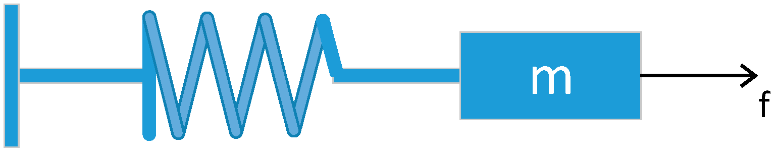
As an example, here, we use a mass-spring system (Figure 1) with no friction (it can also be seen as a 1-DOF robot) to illustrate the relationship and interconnection between the energy based Lagrange equation and the Lyapunov stability theory.
The goal is to move the mass, m, from position to the desired position, . The equation of motion is known as .
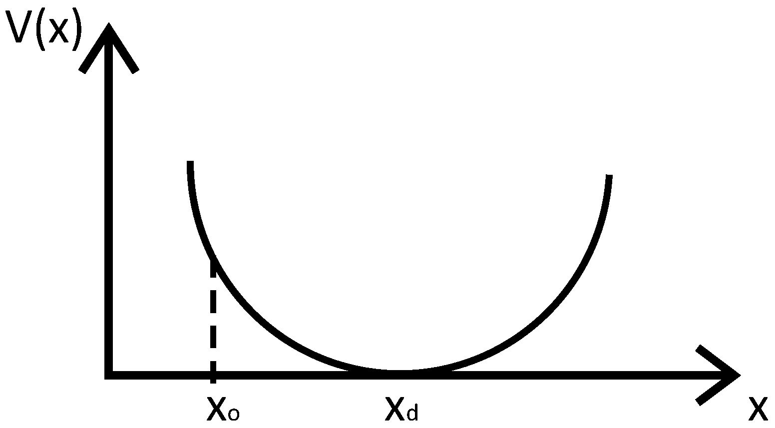
The Lyapunov candidate function, , is chosen as , and , and therefore we have . Figure 2 shows that if one considers the Lyapunov stability, it can be seen as a parabola. The minimum point in the bottom is the stable point, and every point on the parabola tends to approach the stable point.
From the Lagrange equation perspective, we have the Lagrange equation as:
where represents the kinetic energy, with and represents the potential energy. After re-arranging Equation (2), we have the following:
The above Lagrange equation says that the kinetic energy and potential energy are on the left side of the equation, and on the right side of equation, there is no external force, which means the system is stable. To go one step further, even though the system is stable, it is clearly that the system will oscillate. To have an asymptotic stable system, we need to add a damping to the system, i.e.,
If , we then will have an asymptotically stable system. For example, one can choose . Thus, we have the control as follows, , i.e., the PD control.
The reason that the PD controller works is that the it mimics the spring-damper system, and according to the global invariant set theorem, the system can globally tend to the stability point. Here, we will give detailed proof on why PD control works in the position control case. Before proceeding to the following, it should be known that the “I” term in the PID control can actually be seen as adaptive control.
It is known that the PD controller can be described as follows:
where , means the actual joint position, and means the joint desired position. Considering the virtual physics, the PD controller can be seen as a virtual spring (P) and virtual damper (D). The reason why the PD controller works can be traced back to Lyapunov theory. The first step here is to have a Lyapunov candidate function as follows:
where represents the inertia matrix. Therefore:
where as a whole means viscous friction. Plugging the control law, , in the above equation, we have:
According to the global invariant set theorem, unless , in other words, unless equals to . This shows that starting anywhere, if we apply the PD controller, the system globally tends to .
2.2. Adaptive Control of Robotic Manipulators
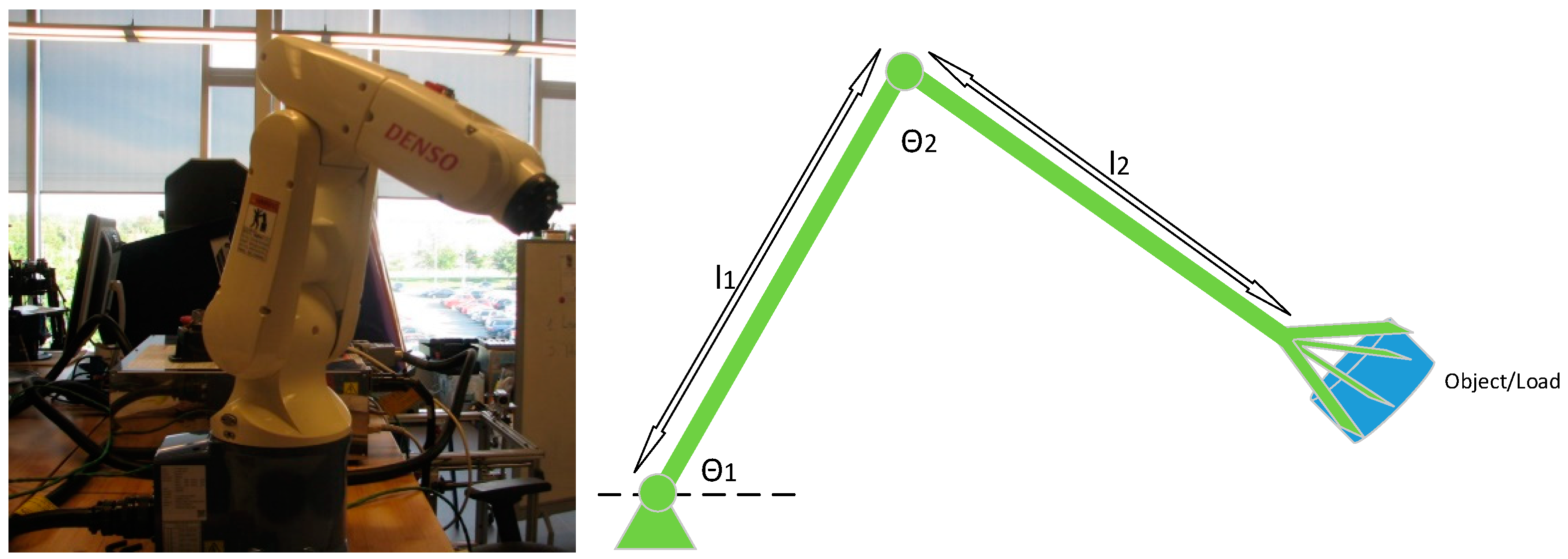
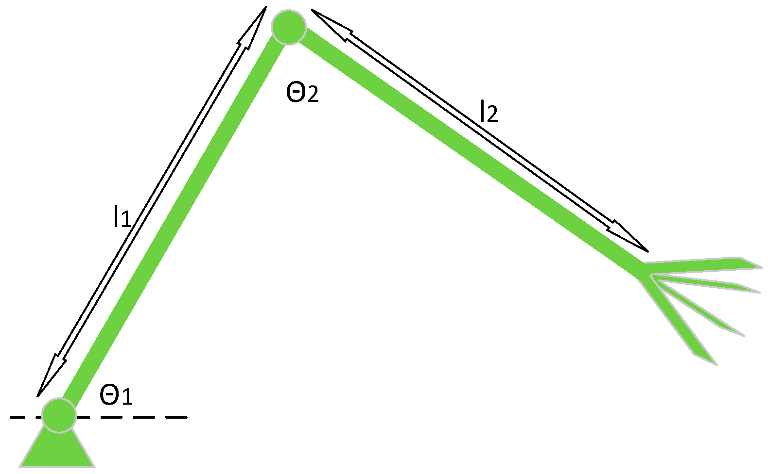
The control issue has been maturely developed in the last decades. PID control (most times PD control) is widely used in industries due to its simplicity. In controlling a robot end-effector position, industries use the PD controller in each joint of a robotic manipulator to control the robot end-effector goal position to accomplish a desired position control. The reason that the PD controller works in controlling a goal position of a robot end-effector in industries nowadays is illustrated above in detail, i.e., it mimics the spring-damper system, and according to the global invariant set theorem (an extended version of the Lyaponuv theorem), the system can globally tend to the stability point. However, if a robot needs to have a specified trajectory or fast motion control, the PD control approach is not good enough to handle the above situations since the PD controller does not tell you what is going on in the process of moving a robot. A more advanced control system is therefore required, for example, adaptive control. As an example, for a 2-DOF serial manipulator with revolute joints, as shown in Figure 3, we have the dynamic equation as follows:
where is the joint angles, is the inertia matrix, is the centripetal and Coriolis torques, is the friction, and is the gravitational torques.
First, the Lyapunov candidate function is chosen as follows:
where and , where is a positive constant number. Then one can calculate as follows:
where is defined as . The above can be written as , where is a known function and is an unknown constant vector, i.e., can be written as a known function times an unknown constant:
By choosing the control law:
where means the estimate of . We have:
It is noted that we have an extra . To eliminate this term, another term, , is added to the above Lyapunov candidate function, then the Lyapunov candidate function can be rewritten as follows:
where is a constant symmetrical positive definite matrix. Then:
where . So, by making the last two terms equal to zero, i.e., by choosing the adaptation law as follows:
Thus, we have:
Based on the Barbalet’s lemma, when and .
2.3. The Role of Friction in Stability Analysis
As an extra note, sometimes the friction is useful in providing a stable condition in the system. The following section will illustrate how friction can be useful in the stability performance. It is known that , so in the dynamic equation, can be written as , thus the dynamic equation can be rewritten as follows:
Instead of throwing away the friction term, as illustrated above, one can use the friction term. In the previous approach, one has . In this case, one has . In the previous approach, , in this case, , and the control law and the adaptation law are therefore as follows:
2.4. Limitations
There are, however, mainly two limitations of the above method: First, it is noticed that in , one assumes that the constant, , does not change with time. This is only valid when changes very slowly with respect to time, then we can assume is constant, or when a robot grasps a load (because the moment when the robot grasps a load, we can assume that the time sets back to zero and becomes constant again). This condition will not be valid in some situations where is changing fast with respect to time (e.g., when a robot performs fast and constant load and unload tasks), if this is the case, then we need to remodel . The second limitation is that the above approach is on the joint space control, as it is known that this requires pre-calculation of the inverse kinematic of the serial manipulators, which is very cumbersome.
The above stability analysis is based on the Lyapunov theory. Another approach in the stability analysis of adaptive control is based on the hyper-stability theory. An example can be found in [25].
2.5. Operational Space Control Case
The drawback of joint space control for a multi-DOF robotic manipulator is that we need to do the inverse kinematic calculation, which is very cumbersome work, as it is known that the inverse kinematic for a serial manipulator is complicated as compared to the forward kinematic calculation. Furthermore, since for the joint space control, first one needs to imagine the final goal position for the end-effector, and then we do the inverse kinematic calculation to determine what the corresponding joint angles need to be. Because of this, another drawback of joint space control is that in real time, when a robotic manipulator meets an unexpected obstacle, one needs to redo the whole motion planning in real time. Due to the above limitations, the operational space control is therefore put forward by Khatib [5].
By applying a force, , at the end-effector, and through multiplying , one can calculate the corresponding joint torque, , needed to achieve the task space control:
In the operational space control, one has motion control and force control. Motion control is to control the motion of the end-effector, and force control is to control how much force the end-effector needs to have. In some situations (e.g., a manipulator cleans a window), motion control and force control need to be considered at the same time. In this way, the effector has the proper force at the effector so that the effector will not break the window. If a robot is interacting with the environment, we must deal with the force control and motion control. A unified motion and force control was studied in [5]. Recent research in [26] was focused on the compliant motion and force control, where the robot end-effector was controlled by the contacting force, and this type of control does not need trajectory planning.
The operational space control has a similar control structure with the joint space control case. The difference is that only the joint variables are changed to the operational space variable. The end-effector equation of motion in the operational space is as follows [27]:
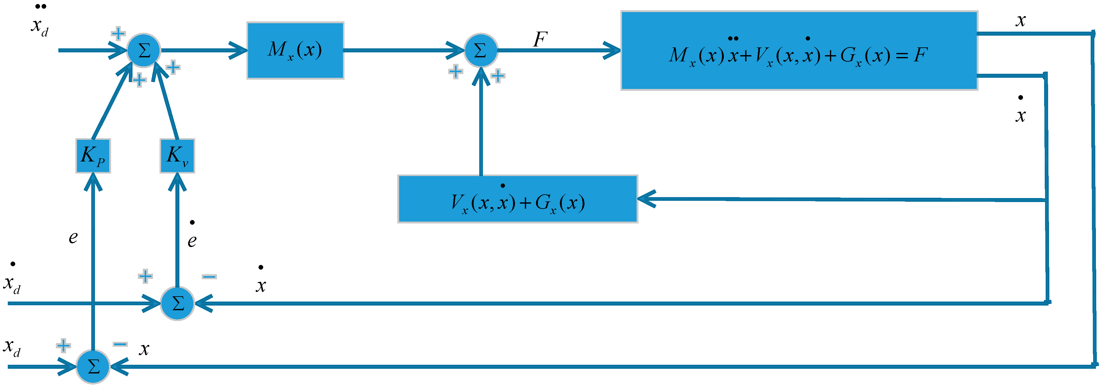
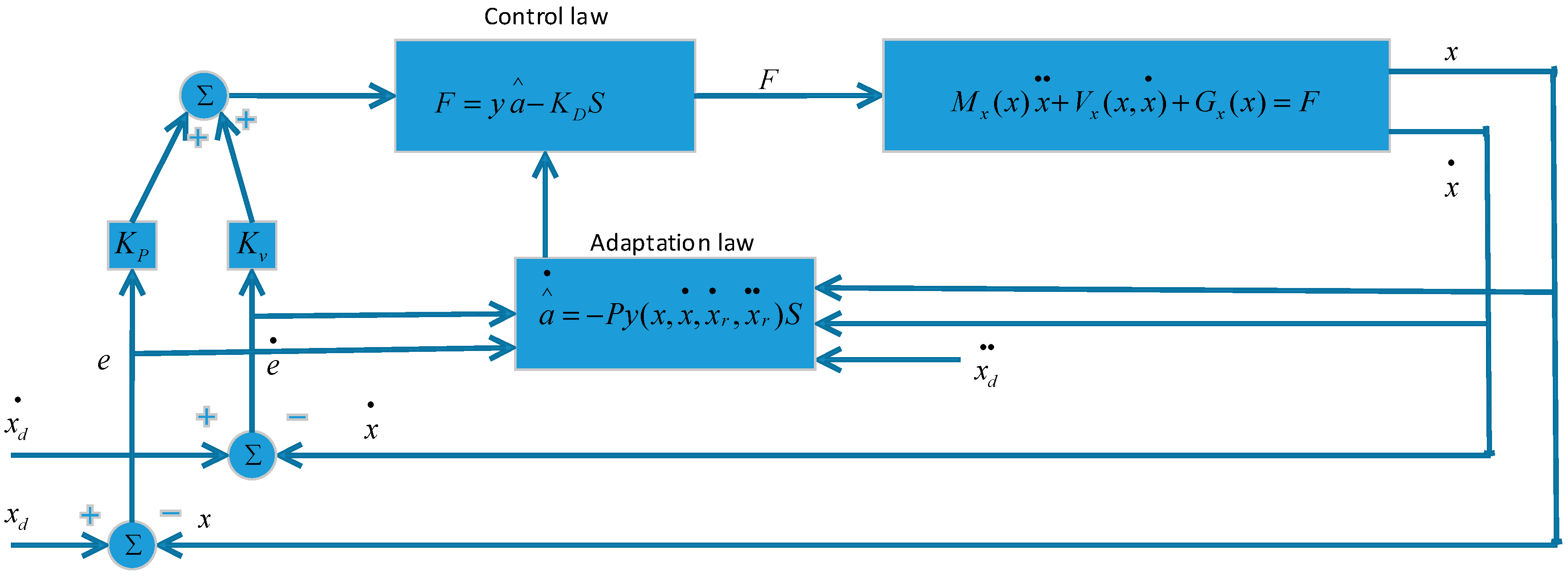
where is the end-effector position and orientation, is the end-effector kinetic energy matrix, is the end-effector centripetal and Coriolis forces, and is the end-effector gravitational forces. By using the decoupling technique, one has the control structure as follows, as shown in Figure 4.
When the end-effector grasps an object to conduct work, it will change the dynamics of the robotic manipulator as the mass and initial properties of the object may be unknown. In this case, we will apply the adaptive control technique. By applying the adaptive control technique, first, the Lyapunov candidate function is chosen as follows:
where and . Then, one can calculate as follows:
where . The above can be written as , where is a known function and is an unknown constant, i.e., can be written as a known function times an unknown constant:
By choosing the control law:
we have:
It is noted that we have an extra . To eliminate this term, another term, , is added to the above Lyapunov candidate function, then the Lyapunov candidate function can be rewritten as follows:
Then:
where . So by making the last two terms equal to zero, i.e., by choosing the adaptation law as follows:
Thus, we have:
Based on the Barbalet’s lemma, when and . The control structure is as follows, as shown in Figure 5.
2.6. Force Control Case
For the force control case, however, it is very different from the motion control case because the dynamic equation is very different. For the motion control case, the dynamic equation is (joint space control) or (operational space control case). We can see that they have the same structure in the dynamic equation. Whereas for the force control case, the dynamic equation is . In the motion control case, when the robot end-effector grasps an object, the unknown parameters are in the or . In the force control case, the unknown parameters are in the .
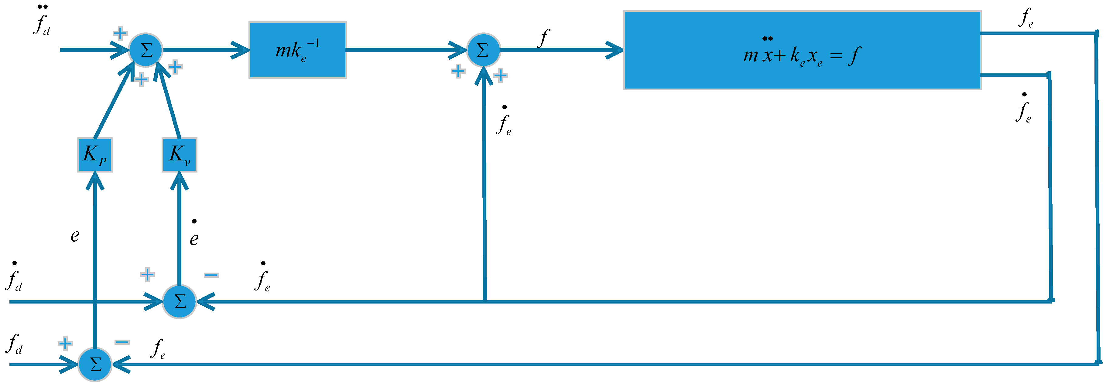
Regarding the force control, in most studies, the controlled force is considered as a constant and does not change with time. Here, the variable force control (force changing with time) is presented. The force equation is:
where is the end-effector/sensor displacement, is the mass of the end-effector, and is the gain of the virtual spring. By using the decoupling technique, one has the control structure as follows, as shown in Figure 6.
Similarly, where the end-effector grasps an object to conduct work, by applying the adaptive control technique, first, the Lyapunov candidate function is chosen as follows:
where and . Then, one can calculate as follows:
where . The above can be written as , where is a known function and is an unknown constant, i.e., can be written as a known function times an unknown constant:
By choosing the control law:
we have:
It is noted that we have an extra . To eliminate this term, another term, , is added to the above Lyapunov candidate function, then the Lyapunov candidate function can be rewritten as follows:
Then:
where . So, by making the last two terms equal to zero, i.e., by choosing the adaptation law as follows:
Thus, we have:
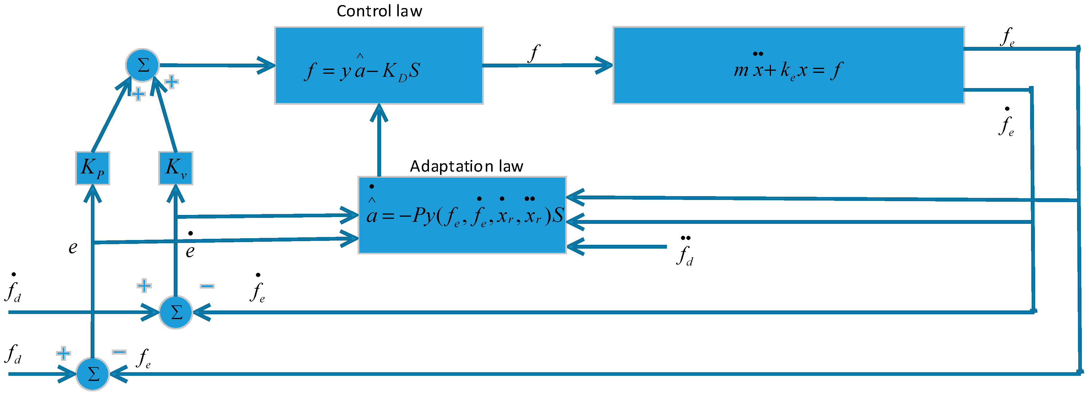
Based on the Barbalet’s lemma, when and . The control structure is shown in Figure 7. The future work will focus on combining the adaptive motion control and force control.
3. Hyperstability Approach
3.1. PID+MRAC Control
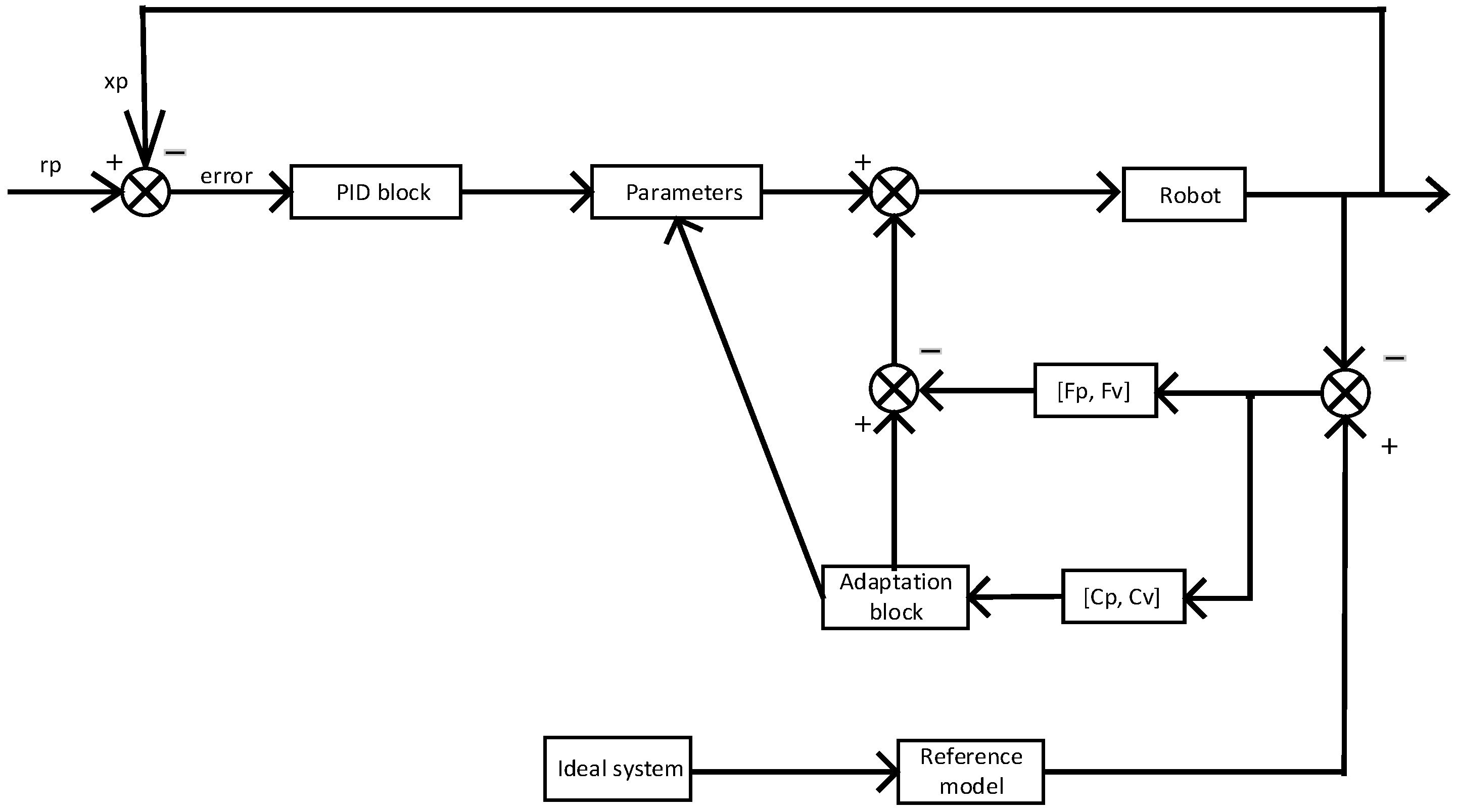
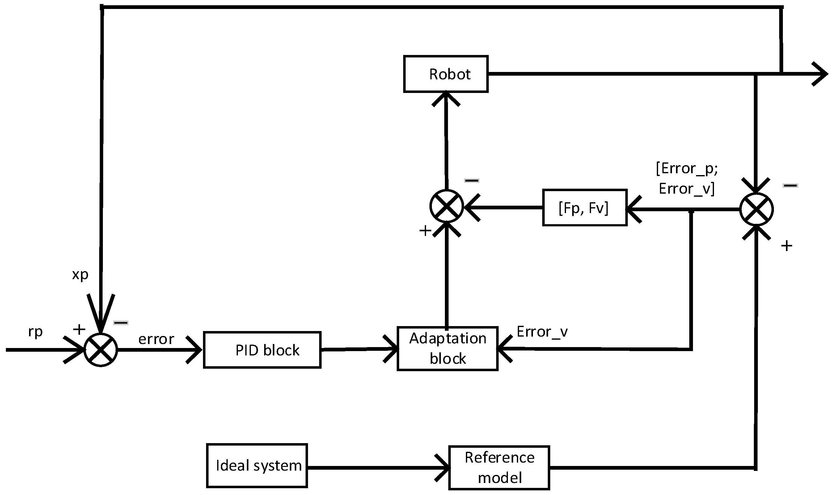
Through incorporating the PID and model reference adaptive controls, a PID+MRAC structure is developed as shown in Figure 8. The synthesis of the PID+MRAC controller is based on the hyper-stability theory. The output from the manipulator compares to the output of the reference model, which will result in a difference. This difference is utilized by the adaptation section to tune the parameters, M and N, matrices of the dynamic model. The matrices, Fp, Fv, Cp, and Cv, are employed for the purpose of making the system stable [6]. In [23], the M and N matrices were treated as constant in the process of adaptation. For the 1-DOF link scenario, it is known that the inertia matrix, M, is not changing and also there is no nonlinear term (i.e., N matrix is zero) in its dynamic formulation, thus one is able to directly combine the PID and the model reference adaptive control system to develop a PID+MRAC controller, as shown in Figure 8. Nevertheless, for the multi degrees-of-freedom scenario, since the M and N matrices of their dynamic formulation are changing when robotic manipulators move and also due to the dynamic equations mismatch, one is not able to combine a PID and the model reference adaptive control directly as in indicated above. On the positive side, however, Sadegh [25] proposed an enhanced version of the model reference adaptive control system that was initially developed in [23], which can combine the PID and the enhanced version adaptive controller, and a combination of PID and the enhanced MRAC is therefore developed for multi degrees-of-freedom manipulators, as shown in Figure 9.
3.2. Modelling and Analysis of One-Linkage Scenario
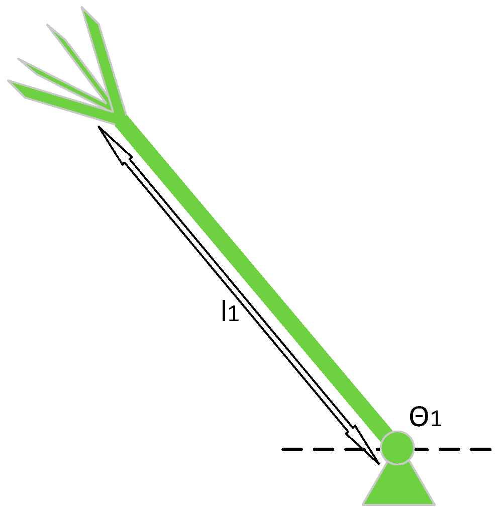
First, a simple one-linkage mechanism (Figure 10) is employed as an example. For the aim of utilizing the PID control for the one-linkage mechanism scenario, the dynamic equation first needs to be modelled and obtained. Based on the Lagrange technique, one has:
where is the link mass, is the angle between the link and x axis, and is the length of the link. By employing the PID, the controller output equals to the torque, i.e.:
where error is . One knows by the one-linkage mechanism’s M and N matrices, the manipulator’s output (i.e., the joint’s acceleration) can be deduced:
Thus, one obtains the joint 1’s acceleration, by taking the integral regarding the time to deduce the joint 1’s velocity and subsequently taking a second integral to deduce the joint 1’s positon.
Regarding the MRAC, in a similar fashion with the PID control, the controller’s output is able to be deduced as following:
where , is the desired input value, and is the actual joint output, please see Figure 9 for reference. and are the parameters that have been adjusted.
The mechanism’s dynamic formulation is:
So, the mechanism’s output (i.e., the joint’s acceleration) is deduced as following:
Furthermore:
where . The first term in Equation (49) is utilized to determine the adaptation algorithm for . The second term is utilized to determine the adaptation algorithm for . and are employed for the purpose of making the system stable according to the hyper-stability theory [6]. By proper selection of the positive definite gain matrices, Fp, Fv, Cp, and Cv, the transfer function, , can be made strictly positive real. Based on the sufficient portion Popov’s asymptotic hyperstability theorem [6], the system is asymptotic stable for all , .
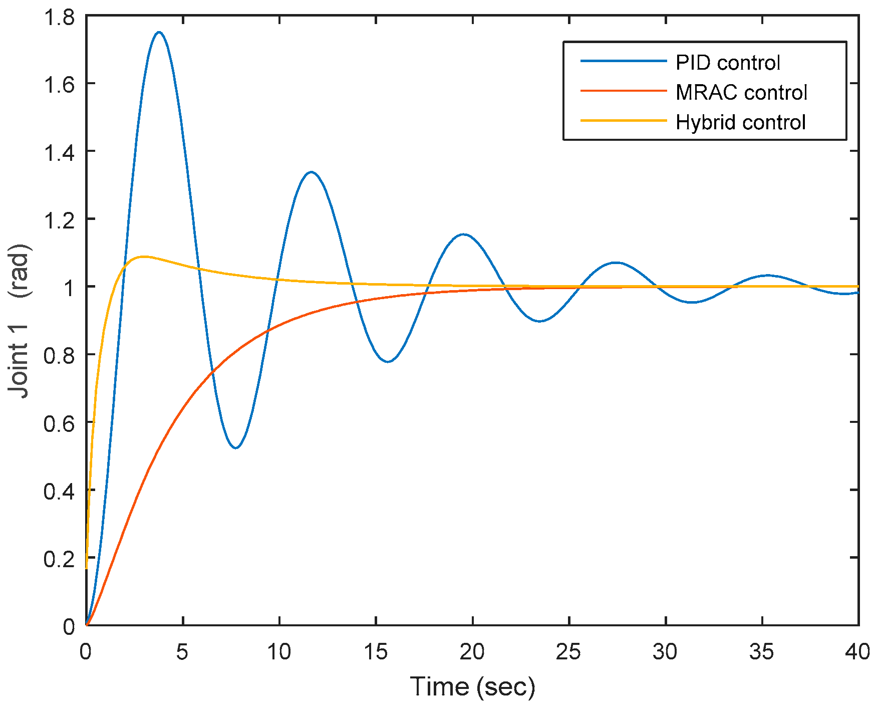
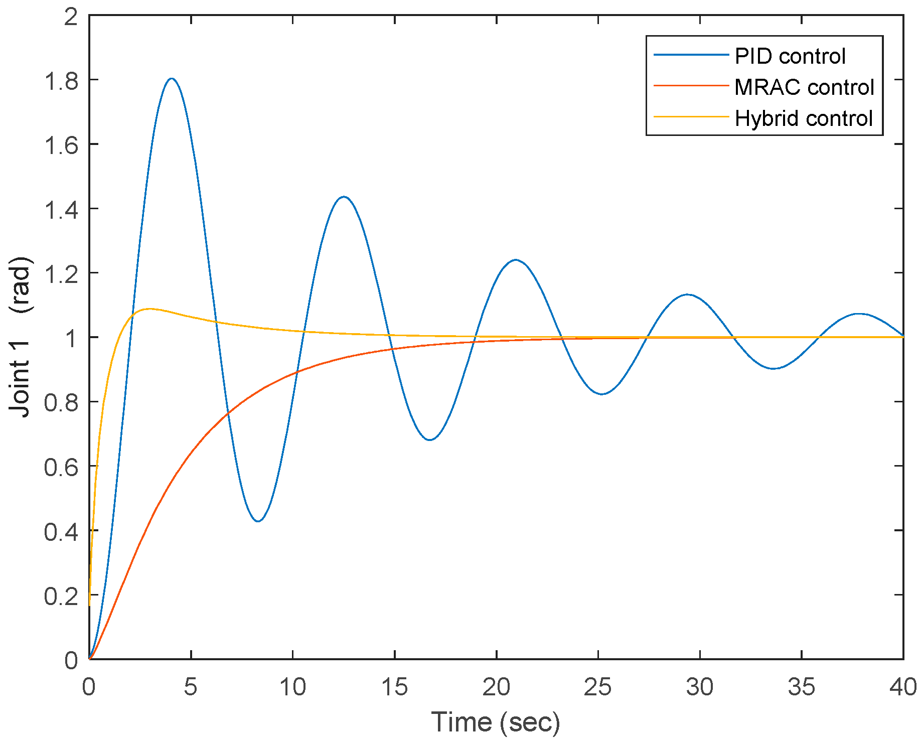
After simulation, as illustrated in Figure 11, the color red in the figure denotes the joint’s output when the MRAC control system is applied, and the color yellow in the figure denotes the joint’s output when the hybrid control is applied, where Cp = 1, Cv = 20, Fp = 20, Fv = 20, adaptation gain is 5, and the proportional gain, integral gain, and derivative gain of the PID part are selected as 5, 1, and 3, respectively. Based on the result, it can be seen that for the PID control, it takes approximately 40 s to converge to zero. The proportional gain, integral gain, and derivative gain are selected as 5, 1, and 3, respectively. With respect to the MRAC system, it takes approximately 20 s to approach the expected spot, and compared to the PID’s case, this is almost half of that period. With respect to the synthesized PID+MRAC system, it takes approximately 10 s to approach the expected spot, and compared to the MRAC’s case, this further reduces to half of that time. In addition, one more difference among the MRAC and the synthesized PID+MRAC systems is that under the MRAC system case, it slowly approaches the expected spot while regarding the synthesized system, it first goes over the expected spot very quickly and then gradually comes back to the expected spot. After multiple tests and choosing different gains, a similar result can be obtained, as shown in Figure 12. Based on previous analysis, it can be seen that the convergent performance under the synthesized PID+MRAC system case beats the MRAC control’s case, and the case under the MRAC system beats the PID system.
3.3. Modelling and Analysis of Two-DOF Link Scenario
Regarding the 2-DOF link scenario (Figure 13), according to the Lagrange technique, the dynamic equation is deduced as the following:
where:
Through re-parametrization of the above formulation:
By choosing , , , one has:
Since:
Thus:
where and represent the joint output position error and velocity error. Once one obtains the joints’ acceleration, taking the integral regarding the time to deduce the joints’ velocity and subsequently taking a second integral to deduce the joints’ positon.
The adaptation algorithm is derived as follows:
So, if one chooses , a stable system can therefore be achieved [6].
Applying the same analysis to the other two terms, the following can be obtained:
The derivation for M is completed, and by resorting to the same technique, one is able to determine the adaptation algorithm for N as follows:
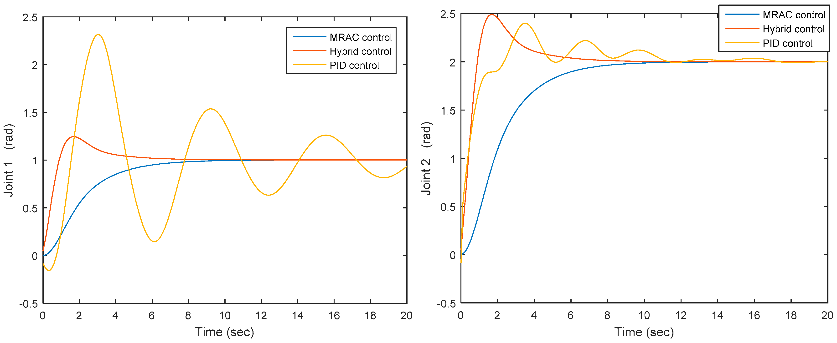
The results show the synthesized PID+MRAC case converges quicker as compared to the model reference adaptive control case, and both the synthesized PID+MRAC and model reference adaptive control cases converge quicker as compared to the PID case, as shown in Figure 14. Through employing the same procedure, it can be extended to the cases where the serial robotic mechanisms have multiple degrees of freedom.
4. Conclusions
The adaptive control design and stability analysis based on two main approaches, i.e., Lyapunov stability theory and hyperstability theory, were studied here. With respect to the Lyapunov approach, the adaptive control of a 2-DOF robotic manipulator was presented. The adaptive control technique was subsequently applied to the end-effector motion control and force control. With respect to the hyperstability approach, a control system was developed through integrating a PID and a MRAC, and also the convergent behavior and characteristics under the situation of the PID, MRAC, and PID+MRAC were compared. The outcome indicates the new enhanced PID+MRAC converges quicker than that of the model reference adaptive control. The experiments and comparisons with other hybrid controllers will be the topic of future work. The experiment will be conducted by using Simulink and dSpace. Motors and motor controllers will be purchased [28], and a multi-DOF serial robot will be set up and built as an illustration. The reason a new robot should be built instead of using a ready-on-market robot is that the control system for most of those robots are built-in controllers.
As an extra note, learning control was developed after the development of adaptive control of robotic manipulators, but it is still in its early development stage. Learning control is used to handle those complex models through learning those complex models, which sometimes have the characteristic of repetitive motions (e.g., most robotic machines used in factories nowadays have repetitive motions) rather than computing them. The main idea behind the leaning control approach is that developing a control approach such that those complex models and uncertainties (e.g., friction at joints) are not needed to model mathematically, but through learning them.
Funding
This research received no external funding.
Conflicts of Interest
The author declares no conflict of interest.
References
- Liang, Q.; Zhang, D.; Wu, W. Methods and Research for Multi-Component Cutting Force Sensing Devices and Approaches in Machining. Sensors 2016, 16, 1926. [Google Scholar] [CrossRef] [PubMed]
- Zhang, D.; Wei, B. Study on Payload Effects on the Joint Motion Accuracy of Serial Mechanical Mechanisms. Machines 2016, 4, 21. [Google Scholar] [CrossRef]
- Li, Z.; Barenji, A.; Huang, G. Toward a Block-chain Cloud Manufacturing System as a Peer to Peer Distributed Network Platform. Robot. Comput. Integr. Manuf. 2018, 54, 133–144. [Google Scholar] [CrossRef]
- Blanes, C.; Mellado, M.; Beltran, P. Novel Additive Manufacturing Pneumatic Actuators and Mechanisms for Food Handling Grippers. Actuators 2014, 3, 205–225. [Google Scholar] [CrossRef] [Green Version]
- Khatib, O. A unified approach for motion and force control of robot manipulators: The operational space formulation. IEEE J. Robot. Autom. 1987, 3, 45–53. [Google Scholar] [CrossRef]
- Landau, Y.D. Adaptive Control: The Model Reference Approach; Marcel Dekker: New York, NY, USA, 1979. [Google Scholar]
- Song, A.; Pan, L.; Xu, G. Adaptive motion control of arm rehabilitation robot based on impedance identification. Robotica 2015, 33, 1795–1812. [Google Scholar] [CrossRef]
- Koivumäki, J.; Mattila, J. Stability-guaranteed impedance control of hydraulic robotic manipulators. IEEE/ASME Trans. Mechatron. 2017, 22, 601–612. [Google Scholar] [CrossRef]
- Xu, G.; Song, A. Adaptive impedance control for upper-limb rehabilitation robot using evolutionary dynamic recurrent fuzzy neural network. J. Intell. Robot. Syst. 2011, 62, 501–525. [Google Scholar] [CrossRef]
- Li, P.; Ge, S.S.; Wang, C. Impedance control for human-robot interaction with an adaptive fuzzy approach. In Proceedings of the 2017 29th Chinese Control and Decision Conference (CCDC), Chongqing, China, 28–30 May 2017; pp. 5889–5894. [Google Scholar]
- Li, Z.; Liu, J.; Huang, Z.; Peng, Y.; Pu, H.; Ding, L. Adaptive Impedance Control of Human–Robot Cooperation Using Reinforcement Learning. IEEE Trans. Ind. Electron. 2017, 64, 8013–8022. [Google Scholar] [CrossRef]
- Sharifi, M.; Behzadipour, S.; Vossoughi, G. Nonlinear model reference adaptive impedance control for human–robot interactions. Control Eng. Pract. 2014, 32, 9–27. [Google Scholar] [CrossRef]
- Dubowsky, S.; Desforges, D. The application of model-referenced adaptive control to robotic manipulators. J. Dyn. Syst. Meas. Control 1979, 101, 193–200. [Google Scholar] [CrossRef]
- Cao, C.; Hovakimyan, N. Design and Analysis of a Novel L1 Adaptive Control Architecture with Guaranteed Transient Performance. IEEE Trans. Autom. Control 2008, 53, 586–591. [Google Scholar] [CrossRef]
- Jain, P.; Nigam, M.J. Design of a Model Reference Adaptive Controller Using Modified MIT Rule for a Second Order System. Adv. Electron. Electr. Eng. 2013, 3, 477–484. [Google Scholar]
- Nguyen, N.; Krishnakumar, K.; Boskovic, J. An Optimal Control Modification to Model-Reference Adaptive Control for Fast Adaptation. In Proceedings of the AIAA Guidance, Navigation and Control Conference and Exhibit, Honolulu, Hawaii, 18–21 August 2008; pp. 1–19. [Google Scholar]
- Idan, M.; Johnson, M.D.; Calise, A.J. A Hierarchical Approach to Adaptive Control for Improved Flight Safety. AIAA J. Guid. Control Dyn. 2002, 25, 1012–1020. [Google Scholar] [CrossRef]
- Li, X.; Cheah, C.C. Adaptive regional feedback control of robotic manipulator with uncertain kinematics and depth information. In Proceedings of the American Control Conference, Montreal, QC, Canada, 27–29 June 2012; pp. 5472–5477. [Google Scholar]
- Rossomando, F.G.; Soria, C.; Patiño, D.; Carelli, R. Model reference adaptive control for mobile robots in trajectory tracking using radial basis function neural networks. Latin Am. Appl. Res. 2011, 41, 177–182. [Google Scholar]
- Sharifi, M.; Behzadipour, S.; Vossoughi, G.R. Model reference adaptive impedance control in Cartesian coordinates for physical human–robot interaction. Adv. Robot. 2014, 28, 1277–1290. [Google Scholar] [CrossRef]
- Ortega, R.; Panteley, E. L1—Adaptive Control Always Converges to a Linear PI Control and Does Not Perform Better than the PI. In Proceedings of the 19th IFAC World Congress, Cape Town, South Africa, 24–29 August 2014; pp. 6926–6928. [Google Scholar]
- Horowitz, R.; Tomizuka, M. An Adaptive Control Scheme for Mechanical Manipulators—Compensation of Nonlinearity and Decoupling Control. J. Dyn. Syst. Meas. Control 1986, 108, 1–9. [Google Scholar] [CrossRef]
- Sadegh, N.; Horowitz, R. Stability Analysis of an Adaptive Controller for Robotic Manipulators. In Proceedings of the 1987 IEEE International Conference on Robotics and Automation, Raleigh, NC, USA, 31 March–3 April 1987; pp. 1223–1229. [Google Scholar]
- Slotine, J.E.; Li, W. On the adaptive control of robotic manipulators. Int. J. Robot. Res. 1987, 6, 49–58. [Google Scholar] [CrossRef]
- Sadegh, N.; Horowitz, R. Stability and Robustness Analysis of a Class of Adaptive Controllers for Robotic Manipulators. Int. J. Robot. Res. 1990, 9, 74–92. [Google Scholar] [CrossRef]
- Sentis, L.; Park, J.; Khatib, O. Compliant control of multi-contact and center of mass behaviors in humanoid robots. IEEE Trans. Robot. 2010, 26, 483–501. [Google Scholar] [CrossRef]
- Craig, J.J. Introduction to Robotics: Mechanics and Control, 3rd ed.; Pearson/Prentice Hall: New York, NY, USA, 2005. [Google Scholar]
- Candelas, F.; García, G.; Puente, S. Experiences on using Arduino for laboratory experiments of automatic control and robotics. IFAC-PapersOnLine 2015, 48, 105–110. [Google Scholar] [CrossRef]
Figure 1.
Mass-spring system.

Figure 2.
Lyapunov candidate function and corresponding state.

Figure 3.
Two-linkage mechanism.

Figure 4.
Decoupling control structure.

Figure 5.
Adaptive control structure.

Figure 6.
Decoupling control structure.

Figure 7.
Adaptive control structure.

Figure 8.
Control system for 1-DOF manipulator.

Figure 9.
Control system for more than 1-DOF linkage.

Figure 10.
One linkage mechanism.

Figure 11.
Joint output under three controls—scenario 1.

Figure 12.
Joint output under three controls—scenario 2.

Figure 13.
Two-linkage mechanism.

Figure 14.
Joints’ 1 and 2 outputs under three controls.

© 2018 by the author. Licensee MDPI, Basel, Switzerland. This article is an open access article distributed under the terms and conditions of the Creative Commons Attribution (CC BY) license (http://creativecommons.org/licenses/by/4.0/).
Share and Cite
MDPI and ACS Style
Wei, B. Adaptive Control Design and Stability Analysis of Robotic Manipulators. Actuators 2018, 7, 89. https://doi.org/10.3390/act7040089
AMA Style
Wei B. Adaptive Control Design and Stability Analysis of Robotic Manipulators. Actuators. 2018; 7(4):89. https://doi.org/10.3390/act7040089
Chicago/Turabian StyleWei, Bin. 2018. "Adaptive Control Design and Stability Analysis of Robotic Manipulators" Actuators 7, no. 4: 89. https://doi.org/10.3390/act7040089
Note that from the first issue of 2016, this journal uses article numbers instead of page numbers. See further details here.