Effects of Land Cover Changes and Rainfall Variation on the Landslide Size–Frequency Distribution in a Mountainous Region of Western Japan

Abstract

This study investigated the size–frequency distribution of 512 landslides triggered by heavy rain in July 2018 on Omishima Island, western Japan. Since the island has undergone rapid land use and land cover changes in recent decades, this study statistically examined the impact of past land cover changes on the shape of, and local variability in, the size–frequency distribution using the inverse gamma model. The possible influence of rainfall conditions was also examined. The landslides were classified based on the severity of anthropogenic disturbance and rainfall using a 56-year (1962–2018) land cover trajectory map and hourly rainfall distribution data. The results indicated that the land cover change (mainly forest conversion into farmland and its abandonment) affected the size and frequency of landslides that occurred decades after the disturbance. Although all landslide groups had similar small rollovers (location of probability peak; 0.042–0.075 × 10⁻³ km²), the scaling exponents of the negative power-law decay were lower for landslides in secondary forest and newly developed farmland (ρ = 1.084–1.231) than in old forest and farmland (ρ = 2.504–2.611). This difference is considered significant compared to general exponent values (ρ = 2.30 ± 0.56), suggesting that farmland development after 1962 caused widespread slope instability, leading to an increase in the proportion of large landslides. By contrast, no clear correlations with rainfall intensity were found, primarily due to complex localised variations in rainfall conditions.

1. Introduction

Landslides are the most prominent erosional process in many mountainous regions [1,2,3] and often cause severe damage [4,5]. To predict the occurrence of landslides and their potential impact on the natural environment and human society in the short (immediately after the occurrence) to the long term, it is essential to quantify and characterise their magnitude and frequency [6,7,8,9,10,11,12,13,14]. Previous landslide studies observed that, above a specific size (landslide slope areas or sediment volume mobilised by landslides), the frequency of landslides decays as a power law [1,9,12,15,16,17,18,19,20,21,22,23]. Below this size, the frequency often decreases, resulting in a transition within the probability density distribution commonly referred to as ‘rollover’. Although the probability density distribution of landslide size is typically similar across regional settings and triggers [9], there is considerable variability in the negative power-law tails and rollovers. This variability might reflect variation in predisposing factors such as geology [15,19,22] and topography [23]. Anthropogenic disturbances are another potential factor altering the size–frequency distribution, as they cause widespread slope instability. Several studies have reported characteristic size–frequency distributions in areas with anthropogenic disturbances [24,25]. However, the anthropogenic influence on the magnitude and frequency of landslides is still not clear, primarily due to the lack of detailed information on spatially heterogeneous land use patterns [25] and the scarcity of landslide inventory data in areas strongly affected by human activities [24]. A better understanding of the factors controlling the shape and variability of the size–frequency distribution is required to use landslide characteristics to detect the effects of environmental changes on slope stability.

Triggering conditions (e.g., variation in rainfall amount, intensity, and duration) should also be considered to explain the landslide size–frequency distribution, as some previous studies have suggested. For example, Alvioli et al. [26] showed that the negative power law of medium-to-large landslides changed with rainfall intensity and duration in physics-based numerical model simulations for given geotechnical parameters. Using cellular automata model simulations, Liucci et al. [27] confirmed that the negative power-law scaling exponent depends on the rate of slope weakening and suggested that the probability density distribution of medium-to-large landslides is likely influenced by rainfall intensity. Although the simulation results from several models highlight the importance of rainfall conditions, few studies have demonstrated changes in the shape of the size–frequency distribution with rainfall variation [21]. Therefore, more studies of the rainfall conditions that significantly affect the number and size of landslides are needed to understand how rainfall conditions systematically change the size–frequency distribution of landslides.

This study investigated the size–frequency distribution of landslides on Omishima Island, western Japan. The island has been widely used as sloped farmland (mainly citrus orchards) [28] but has experienced rapid land use and land cover changes in recent decades [29,30]. Performing statistical analyses using the three-parameter inverse gamma distribution [9], which has been broadly used to characterise landslides and their triggers, this study tested whether the difference in land cover changes preceding a recent storm event and the spatial variation in rainfall influence the size–frequency distribution of landslides. To this end, 512 rainfall-triggered landslides [30] were grouped based on the land cover trajectory pattern and rainfall intensity (rarity) at their respective locations. A land cover trajectory map of the island was used to divide slopes based on the presence or absence of anthropogenic land cover changes and the disturbance period. Hourly rainfall distributions and statistically modelled relationships between rainfall intensity and the return period (RP) were used to analyse the spatial variation in rainfall intensity during a landslide-triggering storm event.

2. Study Area

This study examined Omishima Island (67.5 km²) in the Setonaikai Sea, western Japan (Figure 1A,B). The elevation ranges from sea level to 436 m (the peak of Mt. Washigato; Figure 1B). Hillslopes primarily vary between 5.0° and 45.0°. The Omishima Observatory (Figure 1B), operated by the Japan Meteorological Agency (JMA), recorded a mean annual temperature of 15.4 °C and precipitation of 1218.6 mm from 1991 to 2020.

The land use and land cover of Omishima Island are characterised by sloped farmland. Based on a vegetation map published by the Ministry of the Environment of Japan [31], farmland covers 32.5 km², of which approximately 84% (ca. 27.4 km²) comprised evergreen citrus orchards from the late 1970s to the 1990s. Due to the narrow plains and mountainous topography of the island, citrus orchards are often located on slopes. The remaining slopes are predominantly covered with semi-natural evergreen and deciduous broadleaf forests, with some conifer plantations. The island has experienced rapid land use and land cover changes in recent decades (Figure 1C). Earlier observations allowed the development of a 56-year (1962–2018) land cover trajectory map using historical archives of aerial photographs and revealed that forest area decreased from 1962 to 1981 due to conversion into orchards, while the forest area increased from 1981 to 2018 primarily due to the abandonment of orchards and their return to forest [30].

From 28 June to 8 July 2018, heavy rainfall affected a broad region of western Japan [32,33]. The Omishima Observatory (Figure 1B) recorded total rainfall of 446.5 mm, with the 24-h rainfall reaching 249.5 mm, breaking previous records (Figure 2). This precipitation event triggered numerous landslides (Figure 1D), causing severe damage to property, infrastructure, and citrus orchards [29,34,35]. Based on post-storm aerial photos and satellite image interpretation, Kimura et al. [30] identified 512 new landslides on Omishima Island; most of these occurred in forests and orchards, reflecting the proportions of land use and land cover on the island by area.

3. Data and Methods

3.1. Land Cover Trajectory and Landslide Data

Kimura et al. [30] previously reconstructed the land cover changes in Omishima Island from 1962 to 2018 and identified eight characteristic trajectory patterns (Figure 1C): conversion to farmland (CFAR); conversion to developed land (CDVL); shift to forest (SFOR); shift to shrub land (SSHR); remaining forest (RFOR); remaining shrub land (RSHR); remaining farmland (RFAR); and remaining developed land (RDVL). The farmland in this classification consisted primarily of citrus orchards. Kimura et al. [30] further investigated the occurrence of landslides due to the July 2018 heavy rain based on post-storm aerial photos and satellite image interpretation; they identified 512 new landslides on the island (Figure 1D). Because the images used for visual interpretation were all very high resolution and were taken within days to months after the storm (aerial photos acquired on 23 September 2018 with 0.25-m resolution; satellite images SPOT-6 acquired on 16 July 2018 with 1.50-m resolution), all data, including the smallest landslides (6 m²), were analysed without setting a minimum range for the landslides included in the analysis.

The land cover trajectory pattern of the slope where each landslide occurred was identified by overlapping these maps in the GIS environment (ArcGIS ver. 10.8.1). The landslide scar area measured previously was used to determine the size of each landslide.

3.2. Event Rainfall Data

This study used radar/rain gauge-analysed precipitation (RRAP) data to analyse the spatial variation in short-to-long-term rainfall during the July 2018 storm event. Ground precipitation has been measured since 1976 at the JMA Omishima Observatory [36] in the centre of the island (Figure 1B). With the development of a radar observation network in Japan, rainfall distribution data covering almost the entire Japanese Archipelago are now available. RRAP is one such dataset; it consists of previous 1-h precipitation data with a spatial resolution of 1 km (2006 to present) generated every 30 min using radar estimates and observations by rain gauges throughout Japan. Kimura et al. [30] estimated the RP of 1–264-h (11 days) rainfalls during the July 2018 storm event using generalised extreme value (GEV) distributions fitted on a 47-year (1976–2022) ground precipitation record (Figure 2). They also estimated the event maxima for 1, 3, 6, 12, and 24 h and the total (264 h) rainfall using RRAP data from 0:00 on 28 June to 0:00 on 8 July 2018 (JST) for each 1-km grid cell.

Using the GEV distributions and spatial data of the event maximum rainfall obtained in the previous study, the RP for each 1-km grid cell was estimated to analyse how much rainfall intensity during the storm event varied within the island and to clarify whether such local variation in rainfall influenced the size–frequency distribution of landslides. For this purpose, landslides were classified into those in areas with lighter and heavier precipitation based on the rainfall RP in each location. The details of the classification procedure are described in Section 3.3.

3.3. Classification of Landslides Based on Land Cover Trajectory and Rainfall Distributions

As previously noted, this study examined two questions: were there any differences in the size–frequency distribution of rainfall-triggered landslides among slopes with different land cover trajectory patterns preceding the recent storm event, and did spatial variation in rainfall influence the size–frequency distribution of landslides? To address these questions statistically, as described in Section 3.4, landslides were classified into groups based on the land cover trajectory pattern and rainfall intensity at their locations.

For the first question, landslides were divided into eight vegetation groups according to the land cover trajectory pattern at each location. The shrub (RSHR and SSHR) and developed land (RDVL and CDVL) groups were omitted from further analysis due to the absence or scarcity of landslides. Landslides occurring in forests (n = 289) included those in old forests that remained since before 1962 (RFOR, n = 168) and those in secondary forests that formed after 1962 (SFOR, n = 121). Similarly, landslides occurring in farmlands (n = 200) included those in old farmlands that remained since before 1962 (RFAR, n = 130) and those in new farmlands developed after 1962 (CFAR, n = 70). Kimura et al. [30] previously revealed that secondary forests formed mainly on former farmlands following their abandonment and were concentrated over the 37 years from 1981 to 2018; in addition, most of the new farmlands developed in former forests and were concentrated over the 19-year period from 1962 to 1981. Given these facts, the differences in the size–frequency distribution of landslides between old (RFOR) and secondary (SFOR) forests were assumed to reflect the impact of past farmland development before reverting to a forest on recent landslide occurrence. It was also assumed that the size–frequency distribution of landslides would differ between old (RFAR) and newly developed (CFAR) farmlands, reflecting the impact of new farmland creation since the 1960s on recent landslide occurrence.

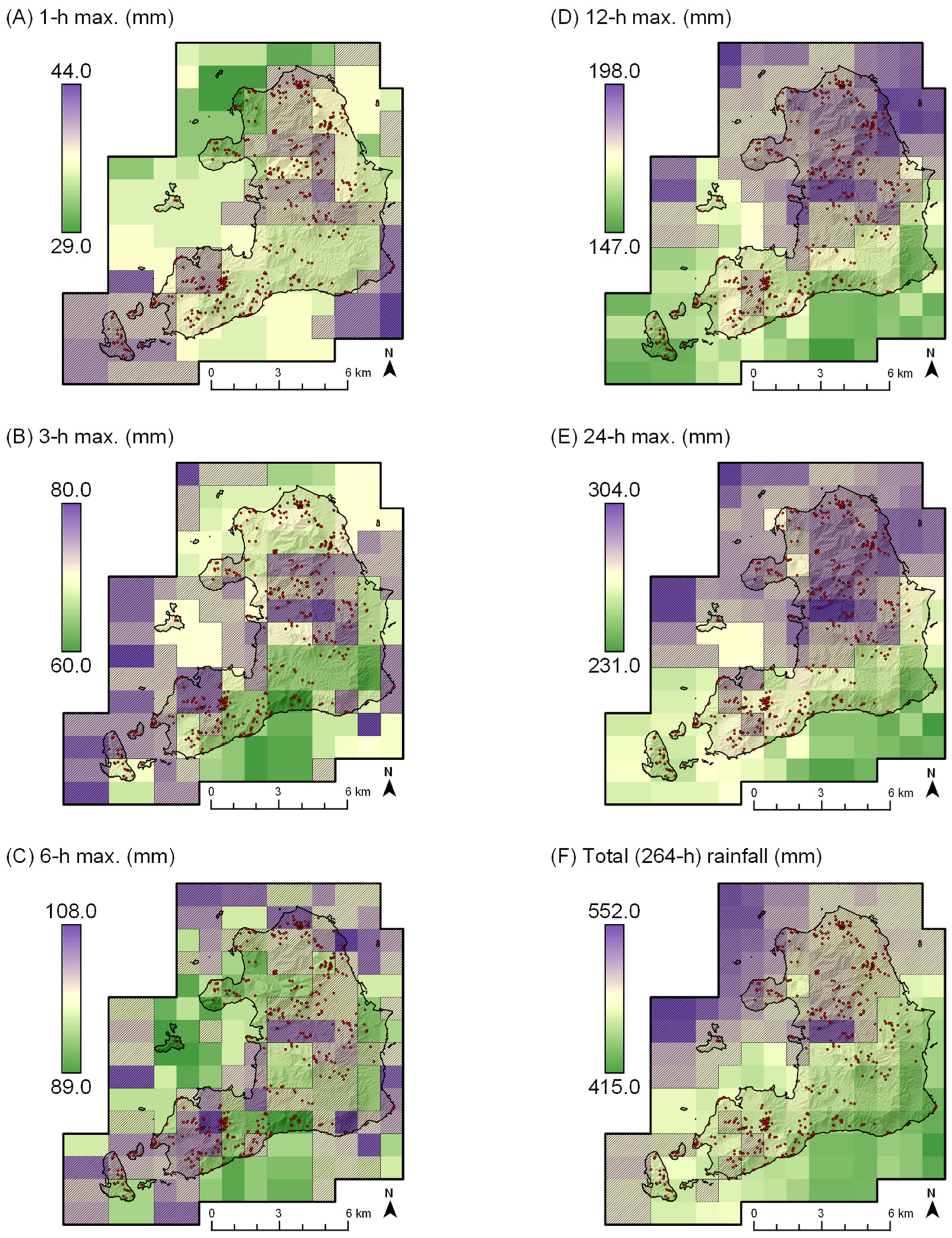
For the second question, the relationship between rainfall intensity and RP was analysed for 1, 3, 6, 12, and 24 h maximum rainfall and the total (264 h) rainfall in the July 2018 storm event. As shown in Figure 3A, the range of rainfall intensity and RP for the 174 grid cells overlapping the study area varied widely depending on the rainfall duration. Therefore, the median value (50th percentile) of the RPs according to the cumulative frequency distribution of each duration was calculated to determine the threshold for classifying the study area into areas with lighter (below 50th percentile) and heavier (above 50th percentile) precipitation (Figure 3B,

Table 1. Statistics of the event maximum rainfall and return periods (RPs) estimated using the distribution of generalised extreme values (GEVs) fit on a 47-year hourly rainfall time series (1976–2022) recorded at the JMA Omishima Observatory.

Rainfall *	5th Percentile **		50th Percentile **		95th Percentile **
	Rainfall (mm)	RP (yr)	Rainfall (mm)	RP (yr)	Rainfall (mm)	RP (yr)
1-h max.	32.0	5.0	36.0	9.0	41.0	19.5
3-h max.	62.0	8.5	70.0	28.1	77.0	143.1
6-h max.	90.0	15.4	97.0	27.1	105.0	55.9
12-h max.	153.0	66.9	174.0	154.6	192.0	318.0
24-h max.	243.0	78.5	271.0	125.4	294.0	176.1
Total (264-h)	433.0	20.8	476.0	33.1	535.0	62.0

Notes: * The event maxima for 1, 3, 6, 12, and 24 h, and the total (264 h), were calculated at each 1-km grid cell of radar/rain gauge-analysed precipitation (RRAP) data overlapping with the study area (174 grid cells in total). ** Respective percentile values were obtained from the cumulative frequency distributions of the 174 grid cells (Figure 3B).

). The landslide data were then divided into those in areas with lighter and heavier precipitation. Figure 4 shows the maximum rainfall distribution and classification results by rainfall intensity (rarity).

3.4. Statistical Analysis for Characterising Landslide Size Distributions

3.4.1. Quantifying Landslide Size Distributions

The non-cumulative frequency density f(A_L) of a landslide inventory is given by the number of landslides δN_L over the range of areas δA_L. The probability density p(A_L) can be estimated as f(A_L) normalized to the total number of landslides N_LT according to:

$$p\left(A_L\right)=\frac{1}{N_{LT}}f\left(A_L\right)=\frac{1}{N_{LT}}\frac{\delta N_L}{\delta A_L}$$

(1)

in which p(A_L) is the probability of a landslide with area A [L²]. The frequency f(A_L) and probability p(A_L) densities of the inventory data were calculated by sorting landslide sizes into bins spaced evenly in logarithmic space.

3.4.2. Landslide Size Distribution Models

A negative power law relationship can express the probability density p(A_L) for medium–large landslides:

$$p\left(A_L\right)=C{A_L}^{-\beta }$$

(2)

where C is a normalisation constant, and β is the scaling exponent of the right tail of the size distribution (β > 1) [18]. This approach requires predefining the size range to fit the model. Because the probability density diverges as A_L → 0, there must be a lower bound to the power law behaviour, which is contained in the normalisation constant, C. To analyse the size distribution considering the total landslide population, Stark and Hovius [17] proposed using a double Pareto model to describe the size distribution of observed landslides, which can quantify not only the negative power law behaviour of medium–large landslides but also the positive power law behaviour of small landslides. In this model, p(A_L) is a function of two scaling exponents, λ and ρ, which describe the rate of decay for small and medium–large landslides, respectively, on either side of a peak landslide area A_Lpeak:

$$p\left(A_L\right)=\frac{\lambda }{A_{L\mathrm{p}\mathrm{e}\mathrm{a}\mathrm{k}}}\frac{{\left[1+{\left(\frac{A_{L\mathrm{m}\mathrm{a}\mathrm{x}}}{A_{L\mathrm{p}\mathrm{e}\mathrm{a}\mathrm{k}}}\right)}^{-\rho }\right]}^{\frac{\lambda }{\rho }}}{{\left[1+{\left(\frac{A_L}{A_{L\mathrm{p}\mathrm{e}\mathrm{a}\mathrm{k}}}\right)}^{-\rho }\right]}^{1+\frac{\lambda }{\rho }}}\times {\left(\frac{A_L}{A_{L\mathrm{p}\mathrm{e}\mathrm{a}\mathrm{k}}}\right)}^{-\left(\rho +1\right)}$$

(3)

where A_Lmax is the largest landslide in the inventory data set, A_Lpeak is the area at which the rollover occurs, λ is the exponent controlling positive power-law scaling when 0 < A_L < A_Lpeak, and ρ is the exponent controlling negative power-law scaling for A_Lpeak < A_L < A_Lmax [17]. Note that the variables labelled α and β in the original paper have been replaced with ρ and λ, respectively, to avoid variable confusion. Thus, the negative power law scaling β in Equation (2) is equivalent to ρ + 1. Similarly, Malamud et al. [9] modelled the probability density of a landslide inventory with a three-parameter inverse gamma function:

$$p\left(A_L\right)=\frac{1}{a\mathsf{\Gamma }\left(\rho \right)}{\left[\frac{a}{A_L-s}\right]}^{\rho +1}\exp \left[-\frac{a}{A_L-s}\right]$$

(4)

where ρ is a parameter controlling the power-law decay scaling for medium–large landslides (again note that β in Equation (2) is equivalent to ρ + 1), a [L²] is a parameter controlling the location of the maximum probability (the peak in the probability distribution), s [L²] is a parameter controlling the exponential rollover for small landslides, and Γ(ρ) is the gamma function of ρ.

In this study, the inverse gamma function of Equation (4) was used to facilitate comparisons with existing landslide studies, while the double Pareto model of Equation (3) was used to visualise the size distribution for the entire dataset.

3.4.3. Statistical Analysis for Model Fitting

To characterise the size–frequency distributions of the landslides triggered by the July 2018 storm event, the frequency f(A_L) and probability p(A_L) densities were calculated following Section 3.4.1 for the entire dataset and subsets grouped by land cover trajectory and rainfall intensity. Then, the model parameters best fitting each dataset were estimated using maximum likelihood estimation (MLE). The goodness-of-fit of the obtained model was evaluated based on the negative log-likelihood value (NLL), Akaike information criterion (AIC), and Bayesian information criterion (BIC). The model uncertainty was shown as the standard error of each optimised parameter, which was taken from the observed information matrix and calculated by numerical approximation. The empirical probability distributions for each pair were compared statistically using the two-sample Kolmogorov–Smirnov (KS) test [37]. These statistical analyses were performed using the MASS package [38] in R ver. 4.2.3.

4. Results

4.1. Size-Frequency Distribution of the Landslides Triggered by the July 2018 Storm Event

The landslide inventory for the July 2018 storm event counted 512 landslide scars on Omishima Island (Figure 1D), with a total area of 0.137 km². According to post-storm field observations, most of the landslides were shallow translational landslides of the topsoil layer [29,30]. Figure 5 shows the size–frequency distribution of these landslides. The median landslide size was 1.21 × 10⁻⁴ km² (121 m²), and the most frequent landslides were on the order of 10⁻⁵–10⁻⁴ km² (10¹–10² m²). The probability density distribution of landslides increased with landslide area, peaking at 0.4–0.8 × 10⁻⁴ km² (40–80 m²) before decreasing in a power-law fashion (Figure 5A). Although rollover occurred at a small landslide size, it is unlikely to be due to under-sampling, as it is one or two orders of magnitude larger than the resolution of the images used for landslide interpretation (10⁻¹–10⁰ m²).

Using MLE, inverse gamma distribution [9] and double Pareto distribution [17] were plotted in Figure 5A. Both models matched the observed probability distribution at areas ≤ 10⁻³ km² (1000 m²), while some discrepancies were observed between the data and model distributions at larger areas (>10⁻³ km²). Figure 5A also shows the general distribution model (a = 1.28 × 10⁻³ km²; s = −1.32 × 10⁻⁴ km²; ρ = 1.40) proposed by Malamud et al. [9]. The peak probability of landslide size for the landslides on Omishima Island was almost an order of magnitude smaller than that of this general model, indicating more frequent small landslides than previously reported in complete landslide inventories associated with a single triggering event. Nevertheless, the negative power-law scaling exponent obtained by fitting the observed probability distribution was close to that of the general model, even when using the inverse gamma (ρ = 1.641 ± 0.141) or double Pareto (ρ = 1.517 ± 0.085) models.

The characteristics of the landslide size distribution in the study area became more prominent when the frequency distribution was compared with those estimated by the general model (Figure 5B). The frequency density of the largest landslides (>10⁻³ km²) in the dataset fell within the range of small-magnitude events (N_LT = 10¹–10²), while that of small–medium landslides (≤10⁻³ km²) varied over a wide range, reaching large-magnitude events at its peak (N_LT = 10²–10⁵).

4.2. Statistical Distribution of Landslides Grouped by Land Cover Trajectory Patterns

To investigate the influence of past anthropogenic land cover changes on the size distribution of recent landslides, subsets of landslide data were analysed according to the land cover trajectory patterns preceding the storm event (Figure 1C). Figure 6 shows the probability density distributions for forest and farmland groups and their inverse gamma models fitted using MLE.

Table 2. Parameters of the inverse gamma models for landslides in areas with different land cover trajectory patterns.

Trajectory Pattern *	Model Parameter **				Goodness-of-Fit ***
	a	s	ρ	Rollover	NLL	AIC	BIC
	(×10−3 km2)	(×10−4 km2)		(×10−3 km2)
Forests (n = 289)	0.194 ± 0.039	−0.164 ± 0.061	1.731 ± 0.208	0.056	1831.858	3669.717	3680.747
RFOR (n = 168)	0.348 ± 0.106	−0.312 ± 0.124	2.504 ± 0.470	0.075	1055.480	2116.959	2126.384
SFOR (n = 121)	0.108 ± 0.032	−0.059 ± 0.067	1.231 ± 0.207	0.042	771.410	1548.820	2125.347
Farmlands (n = 200)	0.140 ± 0.029	−0.133 ± 0.050	1.506 ± 0.192	0.042	1225.985	2457.971	2467.820
RFAR (n = 130)	0.252 ± 0.083	−0.238 ± 0.093	2.611 ± 0.542	0.042	750.746	1507.491	1516.094
CFAR (n = 70)	0.136 ± 0.049	−0.108 ± 0.108	1.084 ± 0.221	0.056	461.448	928.896	935.510
All landslides (n = 512)	0.176 ± 0.025	−0.167 ± 0.041	1.641 ± 0.141	0.056	3215.394	6436.787	6449.502

Notes: * The inverse gamma distribution was fitted to respective size–frequency distributions for landslides in forest (RFOR (remaining forest) and SFOR (succession to forest)) and farmland (RFAR (remaining farmland) and CFAR (conversion to farmland)) areas. ** Three parameters of the inverse gamma distribution are shown with standard error estimates. The rollover value indicates the most frequent landslide size estimated from the probability density distribution model. *** Abbreviations: NLL, negative log-likelihood value; AIC, Akaike information criterion; BIC, Bayesian information criterion.

summarises the optimised parameters and goodness-of-fit of the models.

There was no significant difference in landslide size between old and secondary forests (two-sample KS test: D = 0.092, p-value = 0.585), while the landslide size in newly developed farmlands differed significantly from that in old farmlands (two-sample KS test: D = 0.298, p-value = 7.662 × 10⁻⁴). Similar unimodal patterns were observed in the probability density distributions for all subset data. However, the optimised inverse gamma model differed between old and secondary forests and between old and newly developed farmlands. Comparing the models of landslides in forests, the scaling exponent of the negative power-law decay increased in RFOR (ρ = 2.504 ± 0.470) and decreased in SFOR (ρ = 1.231 ± 0.207), despite having rollovers similar to that of all landslides (0.042–0.075 × 10⁻³ km²). Such model differences became more pronounced between landslides in farmlands (old farmland (RFAR): rollover ≃ 0.042 × 10⁻³ km², ρ = 2.611 ± 0.542; newly developed farmland (CFAR): rollover ≃ 0.056 × 10⁻³ km², ρ = 1.084 ± 0.221). These results suggest that landslides in areas with anthropogenic land cover changes have a lower scaling exponent of the negative power-law decay (more gradual attenuation of landslide frequency) and a proportionately greater number of large landslides.

4.3. Statistical Distribution of Landslides Grouped by Rainfall Intensity

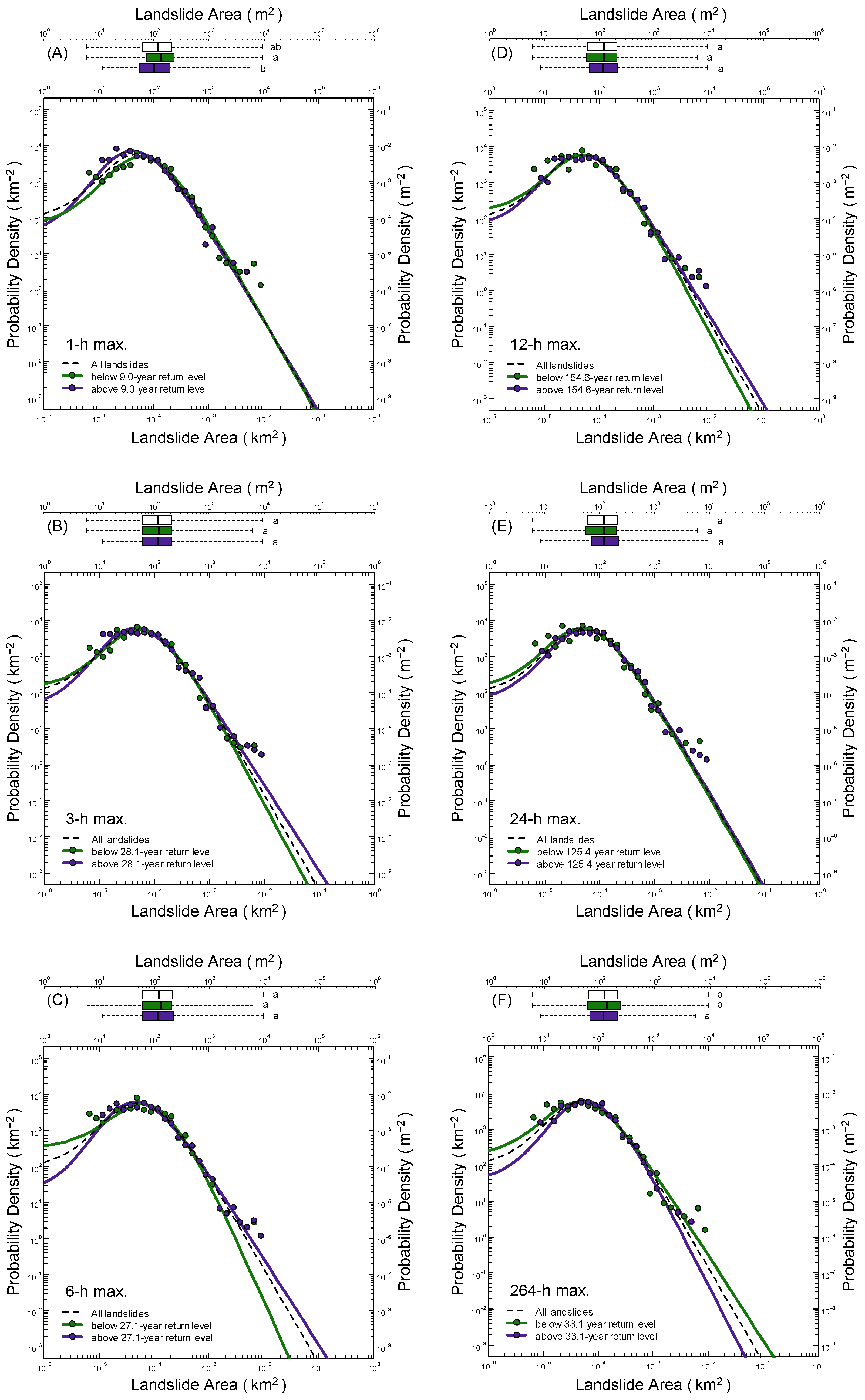
The landslide inventory data were subdivided into landslides in areas with lighter and heavier precipitation based on the rainfall RPs for each rainfall duration (Figure 3 and Figure 4). Figure 7 shows the probability density distribution for each rainfall intensity (rarity) group and its inverse gamma model fitted using MLE.

Table 3. Parameters of inverse gamma models for landslides in areas with different rainfall intensities.

Rainfall *	Model Parameter **				Goodness-of-Fit ***
	a	s	ρ	Rollover	NLL	AIC	BIC
	(×10−3 km2)	(×10−4 km2)		(×10−3 km2)
1-h max.
RP ≤ 9.0 yr (n = 292)	0.212 ± 0.036	−0.193 ± 0.055	1.710 ± 0.183	0.056	1864.621	3735.242	3746.272
RP > 9.0 yr (n = 220)	0.130 ± 0.031	−0.108 ± 0.056	1.535 ± 0.215	0.042	1344.075	2694.150	2704.331
3-h max.
RP ≤ 28.1 yr (n = 305)	0.213 ± 0.040	−0.205 ± 0.059	1.857 ± 0.215	0.056	1900.689	3807.378	3818.539
RP > 28.1 yr (n = 207)	0.136 ± 0.030	−0.120 ± 0.056	1.397 ± 0.182	0.042	1313.215	2632.430	2642.428
6-h max.
RP ≤ 27.1 yr (n = 182)	0.324 ± 0.090	−0.327 ± 0.107	2.430 ± 0.419	0.056	1120.105	2246.210	2255.822
RP > 27.1 yr (n = 330)	0.135 ± 0.024	−0.109 ± 0.044	1.396 ± 0.143	0.042	2091.150	4188.300	4199.697
12-h max.
RP ≤ 154.6 yr (n = 219)	0.210 ± 0.026	−0.205 ± 0.069	1.875 ± 0.258	0.056	1358.028	2722.055	2732.222
RP > 154.6 yr (n = 293)	0.157 ± 0.029	−0.143 ± 0.051	1.504 ± 0.167	0.042	1856.504	3719.009	3730.049
24-h max.
RP ≤ 125.4 yr (n = 234)	0.170 ± 0.036	−0.168 ± 0.058	1.664 ± 0.213	0.042	1455.081	2916.162	2926.528
RP > 125.4 yr (n = 278)	0.181 ± 0.035	−0.163 ± 0.057	1.623 ± 0.188	0.056	1759.397	3524.794	3535.677
Total (264-h)
RP ≤ 33.1 yr (n = 249)	0.144 ± 0.029	−0.159 ± 0.055	1.381 ± 0.163	0.042	1600.017	3206.034	3216.587
RP > 33.1 yr (n = 263)	0.219 ± 0.046	−0.174 ± 0.064	1.998 ± 0.257	0.056	1610.765	3227.530	3238.246
All landslides (n = 512)	0.176 ± 0.025	−0.167 ± 0.041	1.641 ± 0.141	0.056	3215.394	6436.787	6449.502

Notes: * The inverse gamma distribution was fitted to respective size–frequency distributions for landslides in areas with lighter (below the 50th percentile of return periods) and heavier (above the 50th percentile of return periods) precipitation. ** Three parameters of the inverse gamma distribution are shown with standard error estimates. The rollover value indicates the most frequent landslide size estimated from the probability density distribution model. *** Abbreviations: NLL, negative log-likelihood value; AIC, Akaike information criterion; BIC, Bayesian information criterion.

summarises the optimised parameters and goodness-of-fit of the models.

There were no significant differences in landslide size according to rainfall intensity variation, except between areas with lighter and heavier 1-h maximum precipitation (two-sample KS test: D = 0.169, p-value = 0.001). The probability density distributions of all subset data showed similar unimodal patterns characterised by a rollover of 0.042–0.056 × 10⁻³ km² and power-law decays on either side. However, the optimised inverse gamma models differed slightly by subset data. Model differences were most pronounced between landslides in areas with lighter and heavier 6-h maximum precipitation (Figure 7C). Despite having almost the same rollover point, the scaling exponent of the negative power-law decay increased in areas with lighter precipitation (RP ≤ 27.1 yr, ρ = 2.430 ± 0.419) and decreased in areas with heavier precipitation (RP > 27.1 yr, ρ = 1.396 ± 0.143). Another apparent difference was observed for total rainfall (Figure 7F), but the relationship between the scaling exponent and rainfall intensity was the opposite (ρ = 1.381 ± 0.163 for RP ≤ 33.1 yr and ρ = 1.998 ± 0.257 for RP > 33.1 yr) for the 6-h maximum precipitation case.

5. Discussion and Conclusions

Recent landslides on Omishima Island show a humped probability (or frequency) distribution (Figure 5) similar to those of reported landslide event inventories, e.g., [9,18,21]. Although the negative power-law scaling exponent obtained from the observed probability distribution was close to that of the general model proposed by Malamud et al. [9], the rollover was offset towards smaller areas than this general model. These characteristics of the landslide size–frequency distribution may reflect unique regional conditions, including land use and land cover dynamics on the island. In a study investigating the landslide size–frequency distributions in areas strongly affected by anthropogenic disturbances, Van Den Eeckhaut et al. [24] developed a historical landslide inventory for a populated hilly region (gentle slopes generally < 8.5°) in Belgium. They found that recent landslides (10⁻⁴–10⁻¹ km²) triggered by localised human activities had a lower frequency without distinct peaks. Another study in the tropical Andes (predominantly steep slopes > 25.0°) of Ecuador investigated anthropogenic land cover changes and landslide occurrence (10⁻⁵–10⁻² km²) over several decades [25]. It revealed that land cover changes (mainly forest degradation and conversion into farmland) shifted the rollover towards smaller landslides. Considering the slope steepness and landslide size on Omishima Island (slopes primarily from 5.0° to 45.0°, landslide areas from 10⁻⁵ to 10⁻² km², with the mode on the order of 10⁻⁵–10⁻⁴ km²), the results of this study are likely to have many similarities with the rollover shift associated with anthropogenic disturbances observed in the tropical Andes.

However, comparing landslides among the slopes with different land cover trajectories on Omishima Island suggested that the anthropogenic land cover changes influence the size–frequency distribution of landslides differently from the simple rollover shift (Figure 6, Table 2). Despite exhibiting similar small rollovers for all landslide groups (0.042–0.075 × 10⁻³ km²), landslides in secondary forest and newly developed farmland had lower scaling exponents of the negative power-law decay than landslides in old forest and farmland (ρ = 1.084–1.231 and ρ = 2.504–2.611, respectively). This difference is significant compared to the general exponent ρ-value of 2.30 ± 0.56 (range: 1.40–3.50), estimated based on an analysis of global landslide inventories [24]. Therefore, the current findings strongly indicate that anthropogenic land cover changes (forest conversion into farmland) not only alter the number of small landslides but also affect the importance of large landslides. Given that the scaling exponent for old farmland was as high as that for old forest, farmland development after 1962 (mainly sloped orchard fields) might result in widespread slope instability, leading to an increase in the proportion of large landslides. The difference in the scaling exponent also suggests that the impact of past land cover changes may manifest decades later during rare heavy rains. This insight could be crucial for appropriate land management and disaster countermeasures; however, more landslide data and statistical validation are needed to determine how long the anthropogenic influence remains on slopes.

It is important to note that the rollover, which is smaller than the general model, could be attributed to differences in the accuracy of landslide interpretation between the previous and current studies. This study analysed fine-scale landslide data developed using very high-resolution images (with 0.25 and 1.50 m resolutions) taken within days to months after the storm. Furthermore, the shape and location of each identified landslide were verified by comparison with a post-storm topographic map at a 0.5-m resolution [30], enhancing the precision and accuracy of the landslide size. To determine whether the observed rollover shift is due to differences in the dominant landslide mechanism, e.g., [10,12], or the accuracy of landslide interpretation, e.g., [1,17], more detailed analyses are required. These analyses should explicitly address the differences in interpretation accuracy from previous studies. This will be the subject of further research.

This study also examined the possible influence of rainfall conditions on the number and size of landslides. Chen [21] previously investigated the size–frequency characteristics of landslide areas in the Tachia River basin in central Taiwan, which suffered severe damage from the 1999 Mw 7.6 Chi-Chi earthquake and subsequent storm events. Comparing landslide locations with the spatial distribution of maximum hourly rainfall and cumulative rainfall interpolated from several ground-rainfall records, Chen [21] found that the scaling exponent of the negative power-law decay was lower in areas with heavier cumulative rainfall (>400 mm/4 days, ρ = 1.57) than in areas with lighter cumulative rainfall (<400 mm/4 days, ρ = 1.84). Similar to this result, several model simulations showed decreasing trends of the scaling exponent with increasing rainfall intensity [26,27]. However, the size–frequency distribution of landslides on Omishima Island was not clearly correlated with rainfall intensity, while the optimised inverse gamma models differed slightly between subsets (Figure 7, Table 3). For the 6-h maximum rainfall case, it was apparent that the negative power-law scaling exponent increased in areas with lighter precipitation (ρ = 2.430) and decreased in areas with heavier precipitation (ρ = 1.396), suggesting that heavier precipitation (above 27.1-yr RP, >97 mm/6 h) induced more frequent large landslides. The opposite trend was found for total rainfall (ρ = 1.381 and 1.998 for lighter (below 33.1-yr RP, ≤476 mm/11 days) and heavier (above 33.1-yr RP, >476 mm/11 days) total precipitation, respectively). This discrepancy might be due to the difference in spatial variation between short- and long-term precipitation. As shown in Figure 4, areas with heavier 6-h precipitation were scattered throughout the study area and were unrelated to the distribution of total rainfall increasing toward the northwest. Given this complex localised variation in rainfall and the impact of past land cover changes, it is necessary to subdivide the landslide data further and assess the impact of short- and long-term rainfall separately. Future studies should address this by investigating a larger area that includes more landslides in various land cover trajectories and rainfall conditions.

References

- Brardinoni, F.; Church, M. Representing the landslide magnitude-frequency relation: Capilano River basin, British Columbia. Earth Surf. Process. Landf. 2004, 29, 115–124. [Google Scholar] [CrossRef]
- Korup, O.; Densmore, A.L.; Schlunegger, F. The role of landslides in mountain range evolution. Geomorphology 2010, 120, 77–90. [Google Scholar] [CrossRef]
- Larsen, I.J.; Montgomery, D.R.; Korup, O. Landslide erosion controlled by hillslope material. Nature Geosci. 2010, 3, 247–251. [Google Scholar] [CrossRef]
- Petley, D. Global patterns of loss of life from landslides. Geology 2012, 40, 927–930. [Google Scholar] [CrossRef]
- Froude, M.J.; Petley, D.N. Global fatal landslide occurrence from 2004 to 2016. Nat. Hazards Earth Syst. Sci. 2018, 18, 2161–2181. [Google Scholar] [CrossRef]
- Benda, L.; Dunne, T. Stochastic forcing of sediment supply to channel networks from landsliding and debris flow. Water Resour. Res. 1997, 33, 2849–2863. [Google Scholar] [CrossRef]
- Hantz, D.; Vengeon, J.M.; Dussauge-Peisser, C. An historical, geomechanical and probabilistic approach to rock-fall hazard assessment. Nat. Hazards Earth Syst. Sci. 2003, 3, 693–701. [Google Scholar] [CrossRef]
- Fuller, C.W.; Willett, S.D.; Hovius, N.; Slingerland, R. Erosion rates for Taiwan mountain basins: New determinations from suspended sediment records and a stochastic model of their temporal variation. J. Geol. 2003, 111, 71–87. [Google Scholar] [CrossRef]
- Malamud, B.D.; Turcotte, D.L.; Guzzetti, F.; Reichenbach, P. Landslide inventories and their statistical properties. Earth Surf. Process. Landf. 2004, 29, 687–711. [Google Scholar] [CrossRef]
- Katz, O.; Aharonov, E. Landslides in vibrating sand box: What controls types of slope failure and frequency magnitude relations? Earth Planet. Sci. Lett. 2006, 247, 280–294. [Google Scholar] [CrossRef]
- Corominas, J.; Moya, J. A review of assessing landslide frequency for hazard zoning purposes. Eng. Geol. 2008, 102, 193–213. [Google Scholar] [CrossRef]
- Stark, C.P.; Guzzetti, F. Landslide rupture and the probability distribution of mobilized debris volumes. J. Geophys. Res.-Earth 2009, 114, F00A02. [Google Scholar] [CrossRef]
- Bennett, G.L.; Molnar, P.; Eisenbeiss, H.; Mcardell, B.W. Erosional power in the Swiss Alps: Characterization of slope failure in the Illgraben. Earth Surf. Process. Landf. 2012, 37, 1627–1640. [Google Scholar] [CrossRef]
- Corominas, J.; van Westen, C.; Frattini, P.; Cascini, L.; Malet, J.P.; Fotopoulou, S.; Catani, F.; Van Den Eeckhaut, M.; Mavrouli, O.; Agliardi, F.; et al. Recommendations for the quantitative analysis of landslide risk. Bull. Eng. Geol. Environ. 2014, 73, 209–263. [Google Scholar] [CrossRef]
- Sugai, T.; Ohmori, H.; Hirano, M. Rock control on magnitude-frequency distribution of landslide. Trans. Jpn. Geomorphol. Union 1994, 15, 233–351. [Google Scholar]
- Hovius, N.; Stark, C.P.; Allen, P.A. Sediment flux from a mountain belt derived by landslide mapping. Geology 1997, 25, 231–234. [Google Scholar] [CrossRef]
- Stark, C.P.; Hovius, N. The characterization of landslide size distributions. Geophys. Res. Lett. 2001, 28, 1091–1094. [Google Scholar] [CrossRef]
- Guzzetti, F.; Malamud, B.D.; Turcotte, D.L.; Reichenbach, P. Power-law correlations of landslide areas in central Italy. Earth Planet. Sci. Lett. 2002, 195, 169–183. [Google Scholar] [CrossRef]
- Iwahashi, J.; Watanabe, S.; Furuya, T. Mean slope-angle frequency distribution and size frequency distribution of landslide masses in Higashikubiki area, Japan. Geomorphology 2003, 50, 349–364. [Google Scholar] [CrossRef]
- Guzzetti, F.; Ardizzone, F.; Cardinali, M.; Galli, M.; Reichenbach, P.; Rossi, M. Distribution of landslides in the Upper Tiber River basin, central Italy. Geomorphology 2008, 96, 105–122. [Google Scholar] [CrossRef]
- Chen, C.Y. Sedimentary impacts from landslides in the Tachia River basin, Taiwan. Geomorphology 2009, 105, 143–151. [Google Scholar] [CrossRef]
- Hurst, M.D.; Ellis, M.A.; Royse, K.R.; Lee, K.A.; Freeborough, K. Controls on the magnitude-frequency scaling of an inventory of secular landslides. Earth Surf. Dyn. 2013, 1, 67–78. [Google Scholar] [CrossRef]
- Qiu, H.; Cui, P.; Regmi, A.D.; Hu, S.; Wang, X.; Zhang, Y. The effects of slope length and slope gradient on the size distributions of loess slides: Field observations and simulations. Geomorphology 2018, 300, 69–76. [Google Scholar] [CrossRef]
- Van Den Eeckhaut, M.; Poesen, J.; Govers, G.; Verstraeten, G.; Demoulin, A. Characteristics of the size distribution of recent and historical landslides in a populated hilly region. Earth Planet. Sci. Lett. 2007, 256, 588–603. [Google Scholar] [CrossRef]
- Guns, M.; Vanacker, V. Shifts in landslide frequency–area distribution after forest conversion in the tropical Andes. Anthropocene 2014, 6, 75–85. [Google Scholar] [CrossRef]
- Alvioli, M.; Guzzetti, F.; Rossi, M. Scaling properties of rainfall induced landslides predicted by a physically based model. Geomorphology 2014, 213, 38–47. [Google Scholar] [CrossRef]
- Liucci, L.; Melelli, L.; Suteanu, C.; Ponziani, F. The role of topography in the scaling distribution of landslide areas: A cellular automata modeling approach. Geomorphology 2017, 290, 236–249. [Google Scholar] [CrossRef]
- Ehime Prefectural History Compilation Committee (Ed.) Ehime Prefectural History, Regional Geography II (Western Toyo Region); Ehime Prefecture: Matsuyama, Japan, 1986; 890p. (In Japanese) [Google Scholar]
- Kimura, T.; Sato, G.; Ozaki, T.; Thang, N.V.; Wakai, A. Landslide susceptibility in a highly-cultivated hilly region: Artificial slope construction in 1963–1979 and the subsequent 2018 landslide event in Omishima, western Japan. In Natural Geo-Disasters and Resiliency: Select Proceedings of CREST 2023; Hazarika, H., Haigh, S.K., Chaudhary, B., Murai, M., Manandhar, S., Eds.; Springer Nature Singapore Pte Ltd.: Singapore, 2023. [Google Scholar]
- Kimura, T.; Sato, G.; Ozaki, T.; Thang, N.V.; Wakai, A. Land cover trajectories and their impacts on rainfall-triggered landslide occurrence in a cultivated mountainous region of western Japan. Water 2023, 15, 4211. [Google Scholar] [CrossRef]
- Ministry of the Environment of Japan (MOE). Vegetation Map. 2023. Available online: https://www.biodic.go.jp/kiso/vg/vg_kiso.html#mainText (accessed on 10 October 2023). (In Japanese)
- National Research Institute for Earth Science and Disaster Resilience (NIED). Characteristics of Cumulative Rainfall in WESTERN Japan during the Heavy Rain Event of July 2018. 2018. Available online: http://mizu.bosai.go.jp/key/RainJulyH30Accu (accessed on 10 October 2023). (In Japanese)
- Japan Meteorological Agency (JMA). Preliminary Report on Characteristics and Causes of Heavy Rains in “July 2018 Heavy Rains” and Their Causes. 2018. Available online: http://www.jma.go.jp/jma/press/1807/13a/gou20180713.pdf (accessed on 10 October 2023). (In Japanese)
- Ehime University Disaster Investigation Team of July 2018 Heavy Rain (EUDIT). Report on the Disaster in July 2018 Heavy Rain; Ehime University: Matsuyama, Japan, 2019; 379p. (In Japanese) [Google Scholar]
- Mori, S.; Ono, K. Landslide disasters in Ehime Prefecture resulting from the July 2018 heavy rain event in Japan. Soils Found. 2019, 59, 2396–2409. [Google Scholar] [CrossRef]
- Japan Meteorological Agency (JMA). Past Weather Data at the Omishima Observatory. Available online: https://www.data.jma.go.jp/obd/stats/etrn/index.php?prec_no=73&block_no=0732 (accessed on 10 October 2023). (In Japanese)
- Conover, W.J. Practical Nonparametric Statistics; John Wiley & Sons: New York, NY, USA, 1971; 462p. [Google Scholar]
- Venables, W.N.; Ripley, B.D. Modern Applied Statistics with S, 4th ed.; Springer: New York, NY, USA, 2002; 495p. [Google Scholar]
Figure 1.
Maps showing the (A,B) location, (C) land cover trajectory, and (D) landslide distribution of Omishima Island in the Setonaikai Sea, western Japan. (A) The red star indicates the location of Omishima Island. (C) The integrated patterns of land cover trajectory based on the sequence of land cover changed between 1962 and 2018 (after Kimura et al. [30]). RFOR, remaining forest; SFOR, shift to forest; RSHR, remaining shrub land; SSHR, shift to shrub land; RFAR, remaining farmland; CFAR, conversion to farmland; RDVL, remaining developed land; CDVL, conversion to developed land. (D) shows the distribution of 512 landslides triggered by the July 2018 storm event (after Kimura et al. [30]).
Figure 2.
Time series of the annual maxima for (A) 1-h, (B) 3-h, (C) 6-h, (D) 12-h, (E) 24-h, and (F) 264-h rainfall in 1976–2022 recorded at the JMA Omishima Observatory. The white dot in each plot indicates the rainfall in the July 2018 storm event. Red lines show rainfall return periods of 10 (lower dotted), 50 (middle dashed), and 100 (upper solid) years.
Figure 3.
Intensities and return periods for 1-, 3-, 6-, 12-, and 24-h maximum rainfall and total (264-h) rainfall in the July 2018 storm event. (A) Relationships between rainfall intensities and their return periods. (B) Cumulative frequency distributions of rainfall return periods. White dots in each plot indicate the location of the 50th percentile values for 1–264-h rainfalls.
Figure 4.
The 1-km grid rainfall distributions in the July 2018 storm event, generated from RRAP data for (A) 1-h, (B) 3-h, (C) 6-h, (D) 12-h, and (E) 24-h maximum rainfall and (F) total rainfall in the July 2018 rainfall event (264 h from 28 June to 8 July 2018). Red dots indicate the distribution of rainfall-triggered landslides. Hatched areas indicate heavier (above the 50th percentile of return periods) rainfall zones.
Figure 5.
Landslide size–frequency distribution for 512 landslides triggered by the July 2018 storm. (A) Probability density distribution of all landslide scars (grey circles). Solid red and blue lines show maximum likelihood estimation of inverse gamma distribution (a = 0.176 ± 0.025 × 10⁻³ km2; s = −0.167 ± 0.041 × 10⁻⁴ km2; ρ = 1.641 ± 0.141) and double Pareto distribution (ALpeak = 0.083 ± 0.012 × 10⁻³ km2; λ = 2.272 ± 0.260; ρ = 1.517 ± 0.085), respectively. The solid grey line is the general landslide probability density proposed by Malamud et al. [9]. The boxplot indicates the lower and upper quartiles (extent of rectangle) with the median (centre line), while the ends of the whiskers indicate the lowest and highest values. (B) Frequency density distribution of all landslide scars (grey circles). Solid black lines represent the general frequency distribution proposed by Malamud et al. [9] for varying total numbers of landslides NLT (101–106).
Figure 6.
Probability density distributions for landslides in (A) forests and (B) farmlands. The dashed black lines show the inverse gamma distribution model for all landslides, while the solid grey line represents the model for landslides in forests/farmlands. Coloured lines are the results of fitting the probability density for each land cover group to the inverse gamma distribution. Boxplots represent the median (centre line), lower/upper quartiles (extent of rectangle), and lowest/highest values (ends of the whiskers) of landslide area data for each land cover group. Lowercase letters (a–c) beside the boxplots indicate statistical differences in landslide size–frequency distributions examined using the two-sample Kolmogorov–Smirnov test (pairs with significant differences at the 5% level (p-value < 0.05) are shown with different letters).
Figure 7.
Probability density distributions for landslides in areas with lighter (below 50th percentile of return periods) and heavier (above 50th percentile of return periods) precipitation for (A) 1-h, (B) 3-h, (C) 6-h, (D) 12-h, (E) 24-h, and (F) 264-h maximum rainfall in the July 2018 storm event. The dashed black line in each plot shows the inverse gamma distribution model for all landslides. Green and purple lines are the respective results of fitting the probability density for lighter and heavier precipitation groups, respectively, to the inverse gamma distribution. The boxplot represents the median (centre line), lower/upper quartiles (extent of rectangle), and lowest/highest values (both ends of the whiskers) of the landslide area data for each precipitation group. Lowercase letters (a and b) beside the boxplots indicate statistical differences in landslide size–frequency distributions examined using the two-sample Kolmogorov–Smirnov test (pairs with significant differences at the 5% level (p < 0.05) are shown with different letters).