


Algorithmic Geology: Tackling Methodological Challenges in Applying Machine Learning to Rock Engineering


1
NBK Institute of Mining Engineering, University of British Columbia, Vancouver, BC V6T 1Z4, Canada
2
Department of Earth, Ocean and Atmospheric Sciences, University of British Columbia, Vancouver, BC V6T 1Z4, Canada
*
Author to whom correspondence should be addressed.
Geosciences 2024, 14(3), 67; https://doi.org/10.3390/geosciences14030067
Submission received: 14 January 2024
/
Revised: 25 February 2024
/
Accepted: 28 February 2024
/
Published: 4 March 2024
(This article belongs to the Special Issue Machine Learning in Engineering Geology)
Abstract
:Technological advancements have made rock engineering more data-driven, leading to increased use of machine learning (ML). While the use of ML in rock engineering has the potential to transform the industry, several methodological issues should first be addressed: (i) rock engineering’s use of biased (poor quality) data, resulting in biased ML models and (ii) limited rock mass classification and characterization data. If these issues are not addressed, rock engineering risks using unreliable ML models that can have potential real-life adverse impacts. This paper aims to provide an overview of these methodological issues and demonstrate their impact on the reliability of ML models using surrogate models. To take full advantage of the benefits of ML, rock engineers should make sure that their ML models are reliable by ensuring that there are sufficient unbiased data to develop reliable ML models. In the context of this paper, the term sufficient retains a relative meaning since the amount of data that is sufficient to develop reliable a ML models depends on the problem under consideration and the application of the ML model (e.g., pre-feasibility, feasibility, design stage).
1. Introduction
Machine learning (ML) has become unavoidable in rock engineering, with academics and industry professionals increasingly incorporating ML into their projects. As with any new tool, its increasing popularity has increased ML methodological issues, such as failing to split the data into a train and test split, using subjective data, and working with extremely limited datasets. A summary of recent ML applications to rock mass characterization and classification data, including concerns with their methodology, is provided in Appendix A and demonstrates the need for a critical discussion on the topic of ML in rock engineering. While other industries have similar problems, they are working towards bringing awareness and finding solutions. Rock engineering, on the other hand, continues to overlook these problems, which has the potential to result in unreliable ML models. In this context, reliable is defined as providing consistently good quality results; therefore, a reliable ML model is an ML model that provides consistently good quality results. A reliable ML model requires high quality (unbiased) data to develop a model that offers accurate predictions, as compared to the “ground truth” or targets, and a sufficient quantity of this high-quality data in order to provide consistent results as measured by an appropriate performance metric [1]. To date, there has been limited discussion on the impacts of poor quality, biased data in insufficient quantities for the development of ML models in rock engineering. The resulting unexplainable or even poor model performances have the potential to hinder the adoption of ML in rock engineering. This paper aims to provide an overview of these methodological issues and, using synthetic data and surrogate modeling, demonstrate their impact on the reliability of ML models. The code and data used in this paper can be found at the following link: https://github.com/beverlyyang/geosciences-machine-learning-in-engineering-geology.
Key Definitions
Before proceeding with the discussion, terminology used in ML and statistics is clarified, as common usage in rock engineering sometimes deviates from the precise definitions:
- Imbalanced data: the distribution of classes or bins is not equal [2]. Note that if a continuous variable is binned, the resulting distribution can be imbalanced, although the severity of the imbalance would depend on the bin width chosen.
- Skewed data or distribution: a distribution of data points in a dataset that is not symmetric around the dataset’s mean [3].
- Outliers: broadly defined as data points that differ significantly from other observations (e.g., data points found in the tail of a distribution). However, there is no set mathematical or statistical definition of what constitutes an outlier [4].
- Training and test data: as part of the machine learning workflow, the dataset is split into its training and test data (referred to as the train/test split in this paper). The ML model is first trained on the training data, then the trained model is evaluated on the test data to better understand how well the model will perform on data it has not seen before. The dataset is often randomly shuffled before its train/test split to ensure that the training and test data have the same distribution. The train/test split serves to evaluate the ability of a machine learning model to perform effectively on new and unseen data. Additionally, this practice helps us to identify and reduce the risk of overfitting, a scenario in which a model excels in accurately predicting outcomes based on the training data but struggles to generalize its predictions to new instances (see below).
- Validation data: the training dataset is split into training and validation data. The model is trained on the training data and then refined or tuned on the validation data before being evaluated on the test data. Including a validation dataset provides a more robust method of evaluating the model performance. When working with smaller datasets, a single train/validation split may misrepresent the test data, so it is often recommended that cross-validation be performed. In cross-validation, the training set is divided into k number of folds (five and ten folds are commonly used) and each fold takes a turn at being the validation set. A validation score is determined for each fold, and the scores for all folds are then averaged to determine an average validation score [1].
- Overfitting: the ML model cannot generalize well as it is too complex and fits to the noise in the data. Overfitting can be identified when the model performs significantly better on the training data than the test data and commonly occurs in smaller datasets [5].
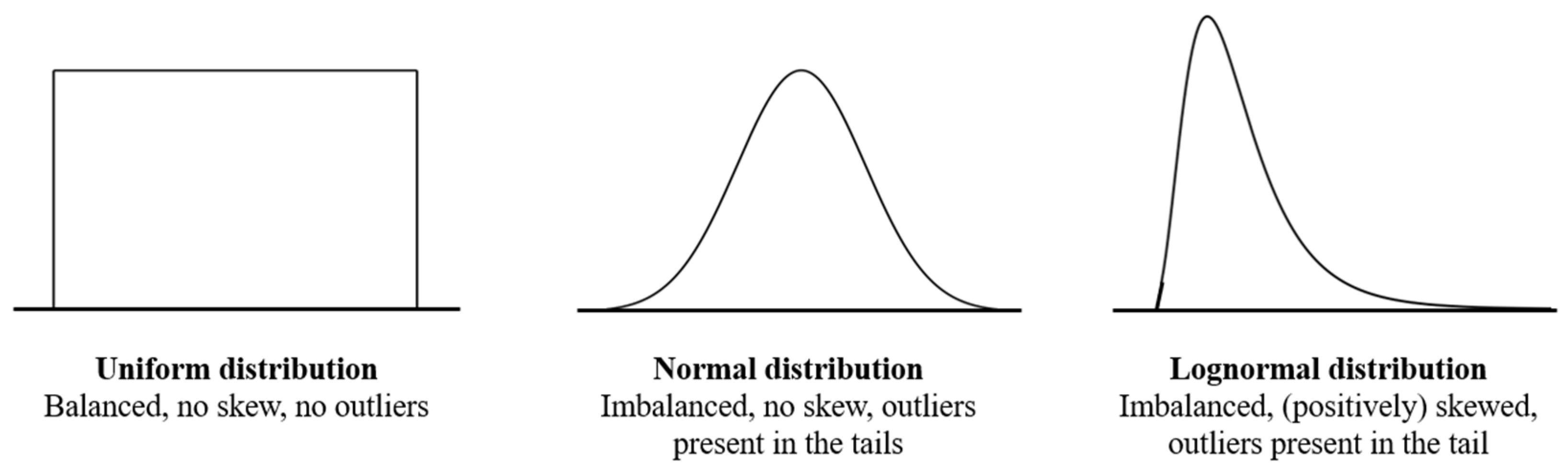
While the terms imbalanced and skewed data are often used interchangeably, it is important to differentiate between them as different techniques are used to handle them. Figure 1 depicts a uniform, normal, and lognormal distribution and describes their distribution characteristics.
2. Data Quality Issues
In machine learning and numerical modeling, incorrect or poor-quality input will result in a misleading output. Likewise, if the data used to develop the model are biased, then the model’s results will be biased [6]. Examples of this include Amazon’s ML recruitment algorithm, which was trained on resumes submitted mostly by men, leading to a gender bias in its predictions, as well as the Correctional Offender Management Profiling for Alternative Sanctions, which was an algorithm used in criminal sentencing to predict which people are most likely to re-offend, that was trained on incomplete data with race as an input, resulting in a racial bias in its predictions [6,7]. Contrary to popular belief, rock engineering also suffers from biased and subjective data; many of the rock mass characterization and classification parameters collected during a site investigation (e.g., rock quality designation, rock mass rating, Q-system, and geological strength index) are subjective and imprecise [8,9,10,11].
These subjective rock mass characterization and classification parameters are common input features and target variables in rock engineering ML applications (e.g., [12,13,14,15], etc.) and their continued inclusion in ML models, as well as the propensity of (often more senior) rock engineering practitioners to blindly and incorrectly believe in their objectivity, pose an obstacle in the development of reliable rock engineering ML models. Additional obstacles to using these parameters in ML include a lack of standardization in collecting them (as each mining and consulting company has its own confidential guidelines), practitioners using them incorrectly, and a general tendency among practitioners to ignore the parameter limitations. The development of reliable ML models in rock engineering requires that rock engineers first acknowledge the subjective and imprecise nature of rock mass characterization and classification parameters, followed by developing more objective parameters that can reliably be used with ML.
3. Data Quantity Issues
The data collection process in rock engineering is often time and cost-intensive and prone to human error due to the nature of the parameters we collect. This can make acquiring good quality data for ML challenging, resulting in smaller datasets relative to other industries. Recent examples of rock engineering ML models have been trained on only a few hundred data points (e.g., [12,13,16,17,18,19], etc.), with some on as few as 80 data points [20]. This starkly contrasts ML models in other industries that have been trained on hundreds of thousands of data and are constantly updating (e.g., NASA’s Prediction of Worldwide Energy Resources). One study, [1], investigated the impacts of data quantity on the performance and reliability of ML models using a synthetic dataset for a slope stability problem. This study demonstrated that ML models trained on smaller datasets can lead to unreliable ML models. More specifically, ML models trained on smaller datasets (i.e., a few hundred data points) are sensitive to how the data was randomly shuffled before its train/test split (controlled by the random_state parameter in scikit-learn’s train_test_split function), resulting in significant variation in both the test R2 and root mean square error (RMSE) for each random shuffling (or random_state value). In other words, how the data were randomly shuffled prior to train/test splitting will have a variable and somewhat random impact on the ML performance.
An example of this variation is shown in Table 1 for a dataset of 250 data points from [1]. A total of 80% of the data was used for training (200 data points), while the remaining 20% was used as the test dataset (50 data points).
This unreliability can also be found using real-world data in rock engineering ML applications. Using the dataset from [12], we developed random forest models with four different random_state values without hyperparameter tuning, with hyperparameter tuning and 10-fold cross-validation via scikit-learn’s RandomizedSearchCV, and with hyperparameter tuning and 10-fold cross-validation via scikit-optimize’s BayesSearchCV. The dataset consists of 138 data points, with 80% used to train the model and the remaining 20% used to test the model. The results in Table 2 demonstrate the variability of the model results depending on how the data were randomly shuffled before the train/test split (i.e., the random_state value).
In previous work by some of the current authors, [1] also noted that ML models developed on smaller datasets can result in overfitting and instances where the model performs better on the test data than the training data, depending on how the data were shuffled before the train/test split (i.e., the random_state value). This study demonstrated that a dataset of 250 data points resulted in overfitting for a random_state of 0, but the model performed better on the test data for a random_state of 42. The ML model performing better on the test data is also found in real-world data such as [12]. The consequence of the model performing better on the test data in datasets with only a few hundred data points is that it can lead to some rock engineers thinking that their model is able to generalize well, when in reality it is most likely an artefact of how the data were shuffled before they were split, and the model is both unable to generalize well and is unreliable.
Of note is that the example in [1] demonstrates more extreme unreliability compared to the results in Table 2. This can be attributed to more extreme outliers in the dataset in [1]; the effect of extreme outliers and skewed data will be discussed in greater detail in Section 3.3 and Section 3.4.
3.1. Methodology
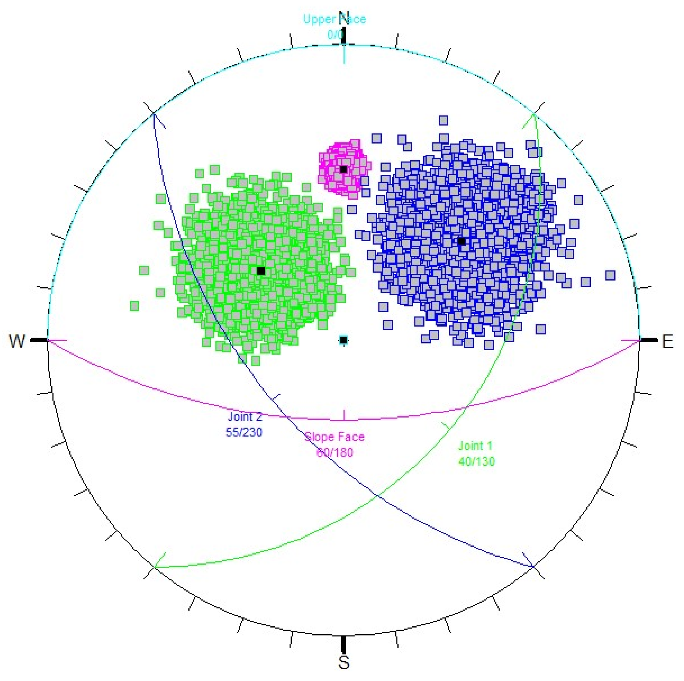
The analysis performed by [1] was expanded to investigate how data preparation and different machine learning algorithms, in conjunction with data quantity, impact the performance and reliability of ML models. The subsequent ML modeling used the same synthetic dataset generated from a SWedge probabilistic analysis [21]. Five thousand data points were generated in SWedge from a Latin Hypercube sampling method with a pseudo-random number generator (using a seed of 1). Any data points where the safety factor was not applicable were removed (8 data points). As noted in [1], surrogate modeling was employed, where the inputs of the SWedge model (the dip and dip direction of the two joints, the friction angle of the two joints, and the dip and dip direction of the slope face) became the input features of the ML model and the target (safety factor) became the target variable of the ML model. Table 3 and Figure 2, taken from [1], show the ranges and distributions of the input parameters of the SWedge and ML model and the stereonet of the two joints and slope faces.
Using the synthetic data, various supervised ML models with different pre-processing steps were developed for varying dataset sizes, ranging from 100 to 4950 data points with a step of 50. Like the methodology outlined in [1], 80% of each dataset was used for training, the remaining 20% was used for testing, and the subsequent training and test scores were determined for each dataset. A 5-fold cross-validation was performed for some of the models with hyperparameter tuning (using scikit-learn’s RandomizedSearchCV and GridSearchCV functions). Four different random_state values (0, 1, 42, and 123) in the train_test_split function in scikit-learn were examined for each model. A learning curve (i.e., dataset size vs. test score) for each random_state value was plotted to examine the impact of the random_state value on the model results and reliability.
The amount of data needed to develop reliable ML models is also dependent on the complexity of the algorithm chosen; more complex algorithms (such as neural networks) will require more data than simpler algorithms (such as linear regression or k-nearest neighbors). As a result, two ML algorithms with varying complexities were examined in the ML modeling: k-nearest neighbors (kNN—a simple, computationally efficient, and easily interpretable algorithm) and multilayer perceptron (MLP—a basic neural network that is better able to identify complex relationships among data compared to kNN). Principal component analysis (PCA) and hyperparameter tuning with 5-fold cross-validation were also performed; hyperparameter tuning for the kNN models was performed with scikit-learn’s GridSearchCV function, while hyperparameter tuning for the MLP models was performed with scikit-learn’s RandomizedSearchCV function. Note that hyperparameter tuning for the MLP models was only performed on dataset sizes of 100, 150, 200, 250, 750, and 2000 for computational efficiency.
The ML modeling consisted of generating regression, classification, and pseudo-regression models. While the target data in this example are numeric and thus appropriate for regression models, the data can be binned into classes for classification models. The data were binned according to the target variable (safety factor) into bins of 0.3 up to a safety factor of 3, and any safety factors greater than 3 were grouped into one bin. Pseudo-regression models can also be developed from the classification models, where the mean of the predicted class is compared with the actual numeric value, and R2 and RMSE can be determined and compared with the R2 and RMSE values from the traditional regression models. Performing classification may reduce the impact of extreme outliers in the target variable, especially in skewed data.
Different methods to handle the imbalanced nature of the target variable were also examined: stratified sampling was performed in the regression and classification models, and data balancing techniques (oversampling and synthetic minority oversampling technique (SMOTE) [22]) were performed in the classification models. Note that oversampling and SMOTE are primarily used in classification problems (such as in the classification models in this paper), however, they have recently been applied to regression problems as well (although they are not as well developed as their classification counterparts). Due to the right skewed lognormal distribution of the target variable, an ln transformation was performed on the target variable for the regression models. This ln transformation was only performed with the kNN algorithm for computational efficiency.
An important aspect to note about ML modeling is the performance metrics used to evaluate the performance and reliability of the models. There are several performance metrics to evaluate regression (as well as pseudo-regression) and classification models, and they may lead to different interpretations regarding the performance and reliability of the models. Common performance metrics for regression and pseudo-regression models are the coefficient of determination R2 and RMSE; while RMSE is more robust than R2, the latter is more commonly used and better understood among rock engineers. Similarly, while the F1-score and AUC (the area under the receiver operating characteristic curve) are more robust performance metrics for classification models (especially for imbalanced data), accuracy is better understood among rock engineers. As a result of this dichotomy between performance metrics, the ML modeling in this paper uses one rock engineering-friendly metric and one robust metric when evaluating the models: R2 and RMSE were used for the regression and pseudo-regression models, while accuracy and F1-score were used for the classification models. To better assess overfitting and the model performing better on the test data, the difference between the train and test accuracy and F1-scores were determined for each dataset size in the classification models. In contrast, only the difference between the test and train RMSE was determined for each dataset size in the regression and pseudo-regression models. The R2 difference was not examined due to the large negative R2 values. The thresholds used to define overfitting in this paper are train–test accuracy ≥ 0.25, train–test F1-score ≥ 0.25, and test–train RMSE ≥ 0.75. Note that these thresholds were arbitrarily chosen for this specific problem.
3.2. Data Visualization
Before implementing machine learning, exploratory data analysis and data visualization should be performed to better understand the data and help guide some pre-processing decisions. The histogram and probability density function of the target variable (safety factor) are shown in Figure 4.
The target variable (safety factor) is both imbalanced and positively skewed. It roughly follows a right-skewed log-normal distribution, which is to be expected for a safety factor distribution for a slope stability problem as the lowest safety factor value is always zero, and its highest value has no limit.
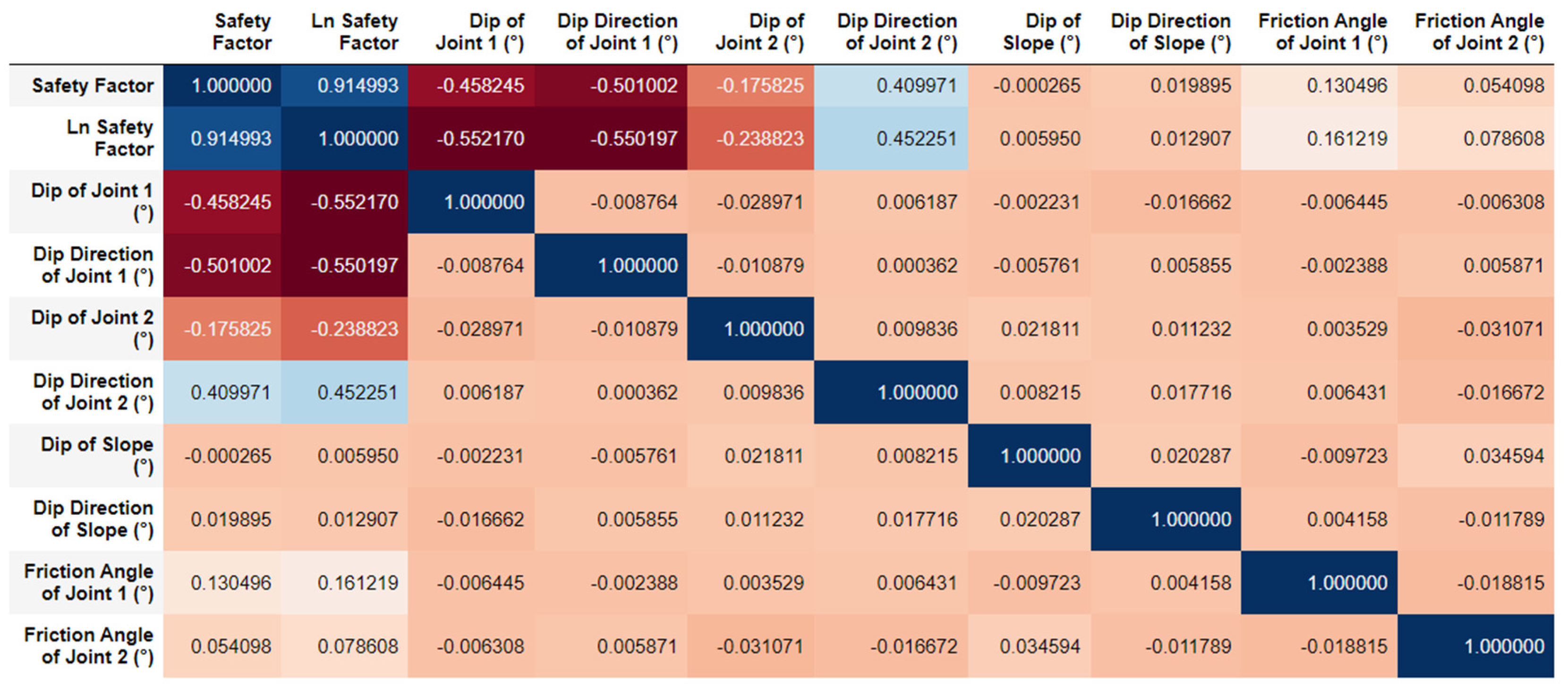
The mean, median, minimum, maximum, and standard deviation of the input features and target variable in the dataset are summarized in Table 6, while the correlation matrix is shown in Figure 5.
The correlation matrix shows that none of the input features are strongly correlated with the safety factor, however, the dip and dip direction of joint 1 show a weak negative correlation to the safety factor, while the dip direction of joint 2 shows a weak positive correlation.
3.3. Results
The learning curves for the base models (Models 1a, 1b, 6a, and 6b) are found in Appendix B (Figure A1, Figure A2, Figure A3, Figure A4, Figure A5 and Figure A6), while the learning curves for the other ML models can be found in the Github link (Section 1). The R2, RMSE, and accuracy learning curves for the base models demonstrate that the models are unreliable at smaller dataset sizes (a few hundred data points) due to their variation depending on the random_state value (i.e., how the data were randomly shuffled before the train/test split). There is less variation between these learning curves for different random_state values after approximately 1500 data points, indicating that there are enough data such that how the data are randomly shuffled prior to data splitting does not significantly impact ML model results. Similar to the other learning curves, the F1-score learning curves also demonstrate that the models are unreliable at smaller dataset sizes, however, the variation between the learning curves for different random_state values is generally smaller than the variation in the accuracy learning curves and remains constant throughout the entire dataset range. The difference between the accuracy and F1-score learning curves demonstrates the importance of the performance metric used in evaluating the model; at smaller dataset sizes (in the order of a few hundred data points), the accuracy learning curves show a more unreliable model compared to the F1-score learning curves, but at larger dataset sizes, the accuracy learning curves show a more reliable model that plateaus at a higher value than the F1-score learning curves. This trend can be seen in the learning curves for the other classification models with different pre-processing techniques and reinforces the importance of choosing an appropriate performance metric.
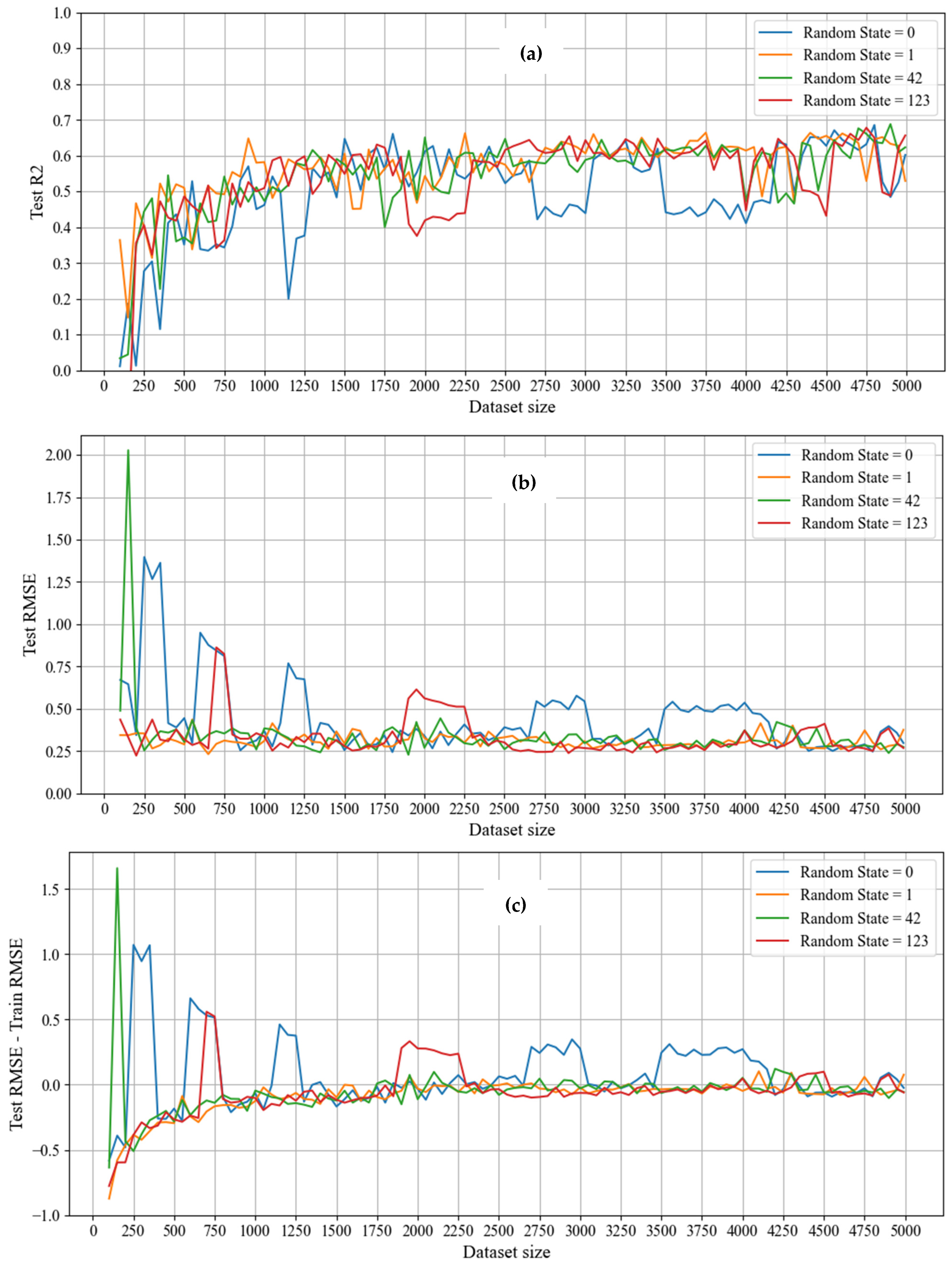
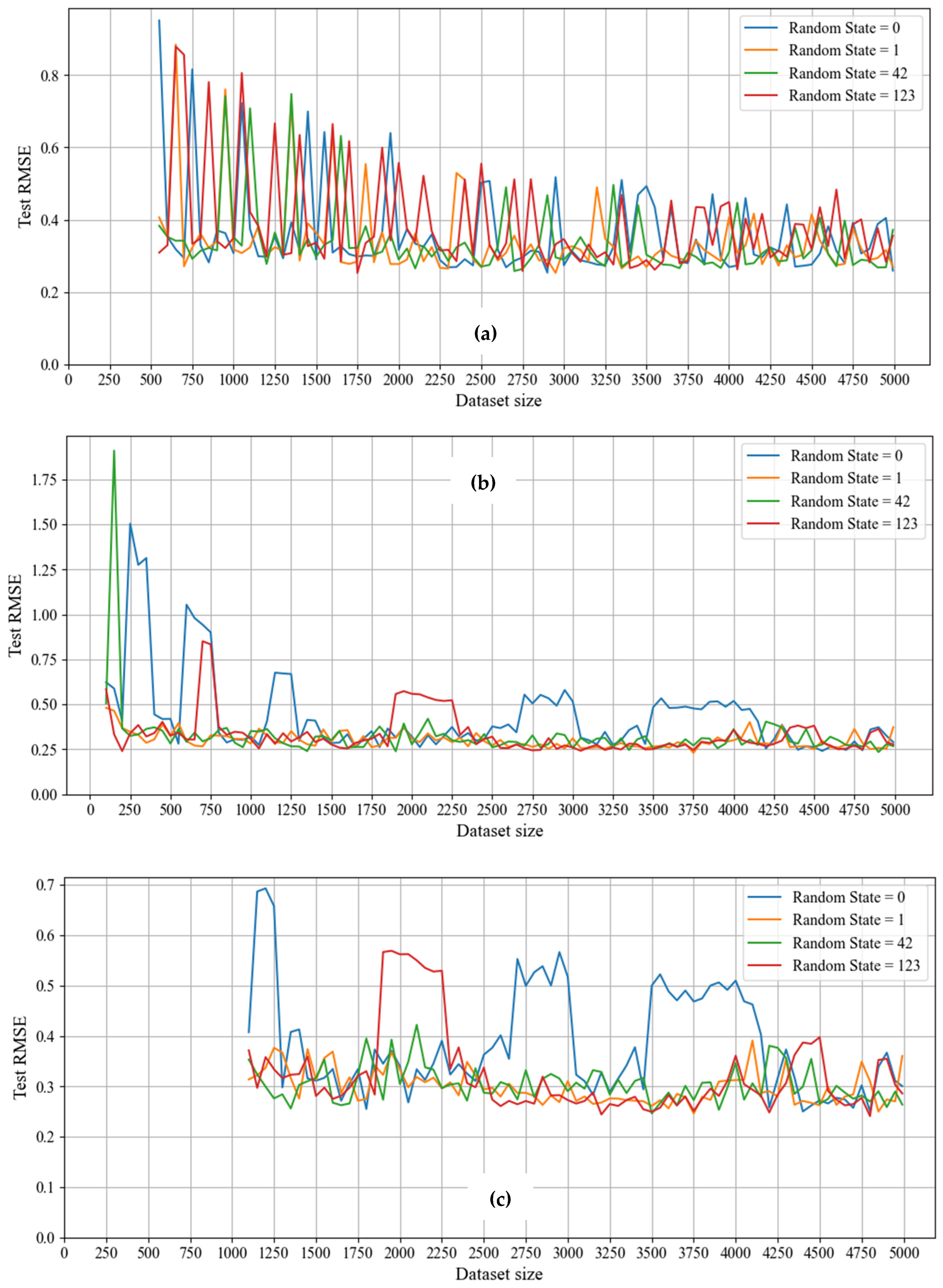
The base model learning curves in Figure A1, Figure A2, Figure A5, and Figure A6 also demonstrate that the unreliability (i.e., variation between learning curves for different random_state values) is more pronounced in regression and pseudo-regression models and can also occur at larger dataset sizes (e.g., at a dataset size of 2000 in Figure A1a, Figure A2a, Figure A5a, and Figure A6a), resulting in the “spikiness” in the learning curves. This spikiness can be attributed to extreme outliers in the dataset and is present in the learning curves for the other regression and pseudo-regression models with different data preprocessing steps. Similarly, overfitting is also generally found in smaller datasets (a few hundred data points) and is more pronounced in the regression and pseudo-regression models. The regression and pseudo-regression models also have more instances of the model performing better on the test data than the training data, compared to the classification models.
Incorporating PCA into the modeling workflow did not improve the reliability of the models compared to their base model counterparts. It had a minimal impact on overfitting and the model performing better on the test data. Hyperparameter tuning with cross-validation also did not improve the reliability of the models (as there is still variation between the learning curves for different random_state values), however, it did reduce the difference between the train and test scores and subsequently overfitting in the MLP classification. Performing hyperparameter tuning in the kNN classification and pseudo-regression models did not impact overfitting. While cross-validation generally provides a more robust evaluation of the ML model than a traditional single train/test split, it is not immune to any extreme values found in the test dataset that are not captured in the training and validation data that lead to unreliable models.
The literature on ML applications in rock engineering tends to focus on neural networks, even when the dataset is small (e.g., [18,23,24]). While neural networks are powerful algorithms that can better identify complex relationships between data than other ML algorithms, they are computationally intensive and require significantly more data than other, simpler algorithms [25]. Due to their data quantity requirements, MLPs and other neural networks may not be the most appropriate algorithm when working with the smaller datasets encountered in rock engineering. This is demonstrated in the learning curves in Figure A2, Figure A4, and Figure A6, as well as the learning curves for the other models; the learning curves for the MLP models are just as unreliable as their kNN counterparts for smaller datasets (less than 750 data points for this example) despite being more computationally intensive and difficult to interpret. Furthermore, the MLP classification and pseudo-regression models result in a more significant difference between the training and test scores in dataset sizes smaller than 250 data points compared to the kNN classification and pseudo-regression models, even after hyperparameter tuning. As a result, the MLP classification and pseudo-regression models developed on dataset sizes smaller than 250 data points exhibit more overfitting than the kNN counterparts. Interestingly, the frequency and magnitude of overfitting are similar for the MLP and kNN regression models, with overfitting occurring at smaller dataset sizes (less than 500–750 data points).
Similar to overfitting, the frequency of the model performing better on the test data is similar between the MLP and kNN regression and pseudo-regression models and occurs across all dataset sizes examined, however, the magnitude of the model performing better on the test data is smaller in the MLP models. Conversely, the MLP classification models did not result in the model performing better on the test data, unlike the kNN classification models that had a few instances occurring in datasets smaller than 1000 data points.
Of note is that the MLP models result in a better performance metric than the kNN models above a certain dataset size (around 1500 data points in this example), thus demonstrating that the MLP models perform better than the kNN models if enough data are available. This improvement is more prominent in the classification models than the regression models (as an example, the kNN and MLP regression learning curves all show spikes at larger datasets), which is most likely due to the extreme outliers in the regression models impacting the MLP and kNN regression models similarly. While the MLP models result in a better performing model than the kNN models at larger dataset sizes, they do not improve the model performance or reliability for smaller datasets, and using MLPs can result in more overfitting in certain scenarios (such as in the classification models in this example) compared to simpler models like kNN.
Comparing the regression, classification, and pseudo-regression models demonstrates that they are all unreliable at smaller dataset sizes (generally a few hundred data points in this example), however, the regression and pseudo-regression models tend to be more unreliable at these smaller dataset sizes (i.e., they have more variation in their R2 and RMSE values for different random_state values for the same dataset) and can also be unreliable at larger dataset sizes (i.e., the spikes in the regression and pseudo-regression learning curves), both of which can be attributed to the increased sensitivity of regression and pseudo-regression models to extreme outliers in the dataset. This sensitivity to outliers in the regression and pseudo-regression models also manifests in increased frequency of overfitting and the model performing better on the test data for the same dataset compared to classification. While the regression and pseudo-regression models are susceptible to outliers in the dataset, the classification models are more susceptible to the choice in the algorithm. The MLP models resulted in better performance metric values than their kNN counterparts when enough data was present, and there were fewer instances of the model performing better on the test dataset than on the training dataset. An important note is that the results of the classification and pseudo-regression models are sensitive to how the data was binned; larger bins (i.e., fewer classes) will result in better classification performance metrics and generally worse pseudo-regression performance metrics, while smaller bins (i.e., more classes) will result in worse classification performance metrics and generally better pseudo-regression performance metrics.
The results of the ML models examined demonstrate the importance of data quantity in developing reliable models. Note that all of the models investigated were supervised models, and the observations in this paper are not applicable to unsupervised models. While the reliability and performance of ML models may be improved by performing classification instead of regression, as well as performing hyperparameter tuning, all of the ML models examined tended to remain unreliable when developed on smaller dataset sizes (a few hundred data points in this example) as they are susceptible to how the data were shuffled before the train/test split (i.e., the random_state value). Overfitting and the model performing better on the test data are also more commonly found in ML models trained on smaller dataset sizes, thus reinforcing the importance of data quantity in ML. It is important to note that the random_state parameter examined in these analyses represents how the data were randomly shuffled before the train/test split and is not a parameter that should be optimized to try to achieve a better model. If the results of an ML model vary significantly depending on the random_state parameter, then that indicates that there is not enough data to develop a reliable model.
3.4. Skewed and Imbalanced Data
Most real-world data are imbalanced, which can negatively impact the results of ML models. There are different approaches to handling imbalanced data, such as stratified sampling—where the class frequencies in the dataset are maintained in the training and test data—and using balancing techniques. The balancing techniques examined in the ML modeling are oversampling (where new samples in the underrepresented classes are generated by randomly sampling from the available data points) and SMOTE (where synthetic data are generated for the underrepresented classes). An example of the learning curves for the models with stratified sampling, oversampling, and SMOTE are shown in Figure A7 and Figure A8.
Due to the nature of stratified sampling and SMOTE, they require a minimum amount of data in each class, resulting in a larger minimum dataset size. As a result, these techniques may not apply to rock engineering datasets that are too small and where the class frequencies are too small. The data balancing techniques (oversampling and SMOTE) did not improve the reliability of the models compared to the base models, as including them in the modeling process did not reduce the variation between the learning curves, especially in smaller datasets. The data balancing techniques slightly increased the difference between the train and test accuracy, F1-score, and RMSE scores, resulting in marginally more instances of overfitting compared to the base models. Similarly, stratified sampling did not significantly impact the models’ reliability, however, unlike the data balancing techniques, stratified sampling reduced the difference between the train and test accuracy, F1-score, and RMSE scores and subsequently reduced overfitting. Both stratified sampling and the data balancing techniques removed the (few) instances of the model performing better on the test data in the classification models.
Another important feature of the target variable distribution is its skewness. Skewed distributions are commonly found in rock engineering. They can significantly impact statistical analyses and machine learning due to the potential for more outliers and more extreme outliers. The safety factor distribution in Figure 4 is a positively skewed (right-tailed) lognormal distribution. Its longer tail contains more extreme outlier values, resulting in spikes in the regression learning curves (Figure A1 and Figure A2). A common method of handling skewed data in regression models is to transform it into a normal distribution. Some examples of commonly used transformations include ln and box cox transformations. However, when evaluating the model, the predicted transformed target variables should be back transformed into the original scale. For this example, an ln transformation was performed on the target variable (safety factor) for the kNN regression model, which had a minimal impact on the learning curves for both the regression and classification models, as shown in Figure A9, Figure A10, Figure A11 and Figure A12. The ln transformation also did not impact the magnitude and frequency of overfitting or the model performing better on the test data when compared to not performing an ln transformation. Another method of handling the extreme outlier values that are commonly found in skewed data is to bin the data and perform a classification (Models 6–11), which reduced the spikes in the learning curves and generally resulted in a more reliable model than performing an ln transformation in the regression model.
3.5. Limitations
Similar to what was noted in [1], the results of the ML modeling performed in this section demonstrate the issues associated with data quantity are specific to the synthetic data generated in SWedge and the ML modeling workflow used. The dataset sizes that result in unreliable ML models in this paper should not be taken as a universal guideline, as they may change depending on the problem, data, and ML methodology. Furthermore, it is worth repeating that the random_state value in scikit-learn’s train_test_split function (i.e., how the data are randomly shuffled before the train/test split) is not a hyperparameter and should not be optimized to obtain a better model. Suppose the results of the ML model vary significantly due to how the data were shuffled before the train/test split. In that case, that indicates that there is not enough data to develop a reliable ML model.
4. Knowledge Issues
A fundamental aspect of developing reliable ML models is ensuring that rock engineers involved in an ML project, from those developing the model to the project managers and senior engineers overseeing the development, have sufficient knowledge of crucial ML concepts and methodological issues. Like other industries outside of computer science/data science that have begun applying ML to their domain-specific problems, rock engineering has a limited number of practitioners who understand ML. This is especially apparent in rock engineering academic publishing; since ML is so new in rock engineering, there are a limited number of experts, making it difficult to find reviewers who are knowledgeable about the topic and leading to flawed methodologies and/or overly complex models developed on simple or data-poor problems being published. For example, ref. [12] developed a model that performs better on the test data and trained the model on incorrect rock mass classification data. Another study, ref. [26], developed models based on their entire dataset instead of splitting the data. Other examples include misunderstandings of ML/statistics-specific terms [27], which led to incorrectly identifying non-normal distributions. As discussed by [28], language is not neutral, and even more important is the perception that specific words leave in the mind of an audience that are neither engineers nor geoscientists. Indeed, in the author’s experience, rock engineering practitioners often misunderstand the terms “validation” and “skewed data”. Potential solutions to these knowledge issues include staffing rock engineering ML projects with data and computer scientists, updating mining and geological engineering curricula to include courses on data science, and mandating that ML publications publish their data and codes so that lessons learned and best practices become easier to access.
5. Conclusions and Recommendations
The development of ML models in rock engineering is not immune to the importance of data quality and quantity. The use of subjective rock engineering parameters in ML models will result in an equally subjective model and model predictions, and the ML models examined in this paper demonstrate that ML models run the risk of being unreliable if they are trained on small datasets, regardless of the data pre-processing steps included in the modeling workflow. This unreliability is exacerbated when extreme outliers are present in the dataset (which tends to occur more frequently in skewed data). It can result in unreliable ML models even when trained on larger dataset sizes. While binning the data to perform classification can help to mitigate the effects of extreme outliers on model reliability at larger dataset sizes, classification models (and pseudo-regression models) are dependent on how the data are binned, and they still result in unreliable ML models when trained on smaller dataset sizes. It is important to remember that the dataset sizes outlined in this paper are specific to this example and there is no universal definition of a small dataset. We recommend that any rock engineers considering applying ML to a problem follow the methodology outlined in this paper and in [1] to determine if there are enough data to develop a reliable ML model. Additional recommendations to ensure the development of reliable ML models in rock engineering include:
- Understanding the methodological issues at play.
- Visualizing the data and performing exploratory data analysis to gain a better understanding of the data.
- Starting simple and increasing the complexity of your model as needed. Increasing the complexity of the model does not necessarily improve the model and is computationally intensive.
If the findings discussed herein are overlooked, ML has the potential to create unnecessary computational expense and model complexity, reinforce and bury data biases, and slow down or even derail engineering decision-making. However, if developed prudently and with an understanding of blind spots in the data, ML is a powerful tool that may be leveraged by rock engineers to relieve the burden of data analysis, uncover hidden data biases, and expedite decision-making.
Author Contributions
Conceptualization, B.Y. and D.E.; methodology, B.Y. and L.J.H.; modeling, B.Y.; writing—original draft preparation, B.Y.; writing—review and editing, B.Y., L.J.H., J.M. and D.E.; supervision, L.J.H. and D.E. All authors have read and agreed to the published version of the manuscript.
Funding
The authors would like to acknowledge the financial support of: Natural Sciences and Engineering Research Council of Canada (NSERC PGS-D), NSERC Grant LJGQ GR000440, and Mitacs Grant POEH/GR022346.
Data Availability Statement
The data used in this study were generated from SWedge and are available from the following link https://github.com/beverlyyang/geosciences-machine-learning-in-engineering-geology.
Conflicts of Interest
The authors declare no conflicts of interest.
Appendix A
Table A1 below provides a summary of recent ML applications to rock mass characterization and classification data, including the concerns with their methodology.

Table A1.
Summary of recent ML applications to rock mass characterization and classification data..
| Reference | Application | Dataset Size | Results | Data and Code Availability | Concerns |
|---|---|---|---|---|---|
| [29] | Used support vector machine and back-propagation neural network to predict basic rock quality (BQ) class from inputs, including JRC, volumetric joint count (Jv), groundwater condition, etc. | 25 data points (20 for training, 5 for test). Also included a separate dataset of 20 data points to “verify” the accuracy of their model. | Accuracy on the 20 data points to “verify” the accuracy of their model is 95%. | The dataset is not available. The code is not available. | Small and imbalanced dataset (BQ class ranges from 3–5, with the majority being 4). The data is limited to Anhui province in China. The ML model is redundant, as many of the input features are used in the equations to calculate BQ class. The training and test accuracy are not reported. |
| [30] | Used naïve Bayes, random forest, artificial neural network, and support vector machine to predict the rock mass rating (RMR) rock mass class from the RMR ratings for intact rock strength, discontinuity spacing, weathering, persistence, aperture, and presence of water. The inputs were label encoded. | 3216 data points (2144 training, 1072 test). The authors performed their own version of cross-validation, where the model was trained 30 times on a different train/test split and the model performance for each split was averaged. | Average test accuracy ranges from 0.81–0.89 for all models. | The dataset is available. The code is not available. | The authors did not make it clear which RMR version was used (RMR89 was assumed). The authors’ version of cross-validation could result in data leakage (where the test data influence the training of the model). The training results were not reported. The models are redundant, as the model inputs make up 68% of RMR89, however, it is possible to estimate the RQD rating from the discontinuity spacing rating since the two parameters are linked, meaning that there is enough information to estimate the RMR class without the use of ML. |
| [12] | Used support vector machine (SVM), decision trees (DT), random forest (RF), Gaussian process regression (GPR), and ensemble learning (EL) using the previous 4 models to predict the end-bearing capacity of rock-socketed shafts from the unconfined compressive strength of intact rock, geological strength index (GSI), length of shaft within the soil layer, length of shaft within the rock layer, and shaft diameter. | 151 data points (121 training, 30 test points). | SVM: training R2 of 0.56, test R2 of 0.55, training RMSE of 2.13, test RMSE of 2.33. DT: training R2 of 0.80, test R2 of 0.85, training RMSE of 1.38, test RMSE of 1.21. RF: training R2 of 0.82, test R2 of 0.87, training RMSE of 1.38, test RMSE of 1.42. GPR: training R2 of 0.79, test R2 of 0.83, training RMSE of 1.50, test RMSE or 1.54. EL: training R2 of 0.84, test R2 of 0.89, training RMSE of 1.39, test RMSE of 1.17. | The dataset is available but contains 138 data points instead of 151. The code is available upon request. | The dataset is small and some of the models perform better on the test dataset than the training dataset. Refer to Section 3 for additional details. |
| [13] | Used relevance vector regression (RVR) and support vector regression (SVR) to predict RMR values from seismic velocity (Vp and Vs), seismic wave type, orientation, polarity, wave magnitude, and reflection depth. | 132 data points (92 training, 40 test). No validation or cross-validation was performed. | RVR: training R of 0.99, test R of 0.94, training RMSE of 1.4, test RMSE of 4.3. SVR: training R of 0.995, test R of 0.96, training RMSE of 1.1, test RMSE of 3.6. | The dataset and code are not available. | The dataset is small and limited—the test RMR values are concentrated between 0 and 20 and 60–85. The data is also based on two case studies in Iran. The RMR version was not specified by the authors. |
| [26] | Used classification and regression tree (CART) as well as genetic programming (GP) to predict tunnel boring machine (TBM) performance (FPI—field penetration index) from uniaxial compressive strength (UCS), rock quality designation (RQD, joint spacing, partial joint condition rating in RMR89, and rock type code. | 580 data points from 7 tunneling projects (4 from Iran, 1 from New Zealand, 1 from India, 1 from Switzerland; 35% metamorphic, 37% igneous, 28% sedimentary). A train/test split was not performed (to the best of my knowledge). | CART: entire dataset R2 of 0.91, entire dataset of RMSE 6.67. GP: entire dataset R2 of 0.85, entire dataset RMSE of 8.46. | The dataset and code are not available. | A train/test split was not performed (i.e., the model results are for the entire dataset), making it difficult to determine how well the models will generalize (which is the end goal of ML). The authors did not explain what a partial joint condition rating from RMR89 meant. |
| [31] | Used k-nearest neighbors (kNN), naïve Bayes (NB), random forest (RF), artificial neural network (ANN), and support vector machine (SVM) to predict rock compressive strength from acoustic characteristics stemming from hitting the core with a geological hammer (amplitude attenuation coefficient (AAC) and high and low frequency ratio (HLFR)). | 2104 data points (1614 training, 400 test). | kNN: training R2 of 0.98, test R2 of 0.98, training RMSE of 0.6, test RMSE of 0.6. NB: training R2 of 0.88, test R2 of 0.88, training RMSE of 3.84, test RMSE of 3.94. RF: training R2 of 0.98, test R2 of 9.07, training RMSE of 1.1, test RMSE of 1.8. ANN: training R2 of 0.99, test R2 of 0.99, training RMSE of 0.3, test RMSE of 0.3. SVM: training R2 of 0.99, test R2 of 0.99, training RMSE of 0.08, test RMSE of 0.1. | The dataset and code are not available. | AAC and HLFR showed good correlation with rock compressive strength without the use of ML (R2 of 0.91 for AAC and R2 of 0.93 for HLFR), putting into question the practicality of using ML for this application. |
| [32] | Used random forest to predict Is50 classes from fracture frequency, RQD, mineralized veins per meter, rock density, intact rock strength hammer test class, alteration strength index, mineralization strength index, mineralization percent sum, fracture spacing, fracture frequency index, discontinuity frequency index, discontinuity frequency index weighted by orientation, joint set index, rock colour, lower contact, rock texture, rock type, selvage mineralization, mineral metric, rock structure, rock fabric, PLT machine ID. | 7687 data points. The authors performed their own version of cross-validation, where their model was trained on all boreholes except for one, and then tested on the remaining borehole. This was repeated until all boreholes had been used as the ”test dataset”, and the score for each borehole was averaged. | The average accuracy of the boreholes is 39%. | The dataset and code are not available. | The authors’ version of cross-validation could result in data leakage (where the test data influences the training of the model). The training results were not reported. Some of the input features are correlated with one another (ex; fracture frequency and fracture frequency index). The reported accuracy is low and does not represent the true “test” accuracy (which should be lower than the reported 39%). |
| [33] | Used stacked autoencoders (SAEs—a type of deep learning) to predict RMR rock mass class from its input parameters (UCS, RQD, spacing, persistence, aperture, roughness, infilling, weathering, groundwater, and orientation). The rating classes of each input parameter was one-hot binary encoded (ex; the UCS rating class for UCS > 250 MPa was transformed into 1000000, while the UCS rating class for UCS between 100 and 250 MPa was transformed into 0100000, etc.) | 309 data points (232 training, 77 test). | The train and test accuracy are both 100%. | The dataset and code are not available. | The dataset is small, especially for a neural network. The model is redundant as it uses the inputs of RMR to determine RMR, which can be done (and is done) easily without ML in Excel. The authors also did not specify which RMR version was used (RMR89 was assumed). The authors also misused the word calibration, as they referred to one-hot encoding the input features as “calibration”, despite it being a form of data preparation. |
| [34] | Used ANN to predict RMR values from its input parameters (strength, spacing, RQD, joint conditions, and groundwater). | The dataset size is unclear. | The MAPE was less than 1%. It was unclear if this was for the training or test set. | The dataset and code are not available. | The dataset size is unclear, and it is unclear if the model performance is for the training or test set. The model is redundant as it uses the inputs of RMR to determine RMR, which can be done (and is done) easily without ML in Excel. The authors also did not specify which RMR version was used (RMR89 was assumed). |
| [18] | Used Gaussian process regression (GPR), support vector regression (SVR), decision tree (DT), and long short-term memory (LSTM—a type of neural network) to predict cohesion and friction angle of sandstone from uniaxial compressive strength, uniaxial tensile strength, and confining stress. | 233 data points from RockData (195 training, 49 test). The authors performed a 5-fold cross-validation. | For cohesion, the R2 of all of the models ranged from 0.95 to 0.98, while the RMSE ranged from 1.3 to 2.38. For friction angle, the R2 of all the models ranged from 0.6 to 0.85, while the RMSE ranged from 1.86 to 9.88. It was unclear if this was for the training set, test set, or entire dataset. | The dataset is available in RockData. The code is not available. | The dataset size is small, especially for LSTM, and limited to only sandstone. It is unclear if the model performance values are for the training set, test set, or entire dataset, making it difficult, if not impossible, to determine how well the model generalizes. |
| [35] | Used convolutional neural networks (CNN) to predict RQD from core photos. | 124 images (99 training images, 25 test images). | Average test error of 3.24%. RQD for training was determined by two experienced engineers. | The dataset is available upon request. The code is available. | The dataset is small, especially for a CNN. The model has issues differentiating between natural and mechanical fractures. The hard and soundness requirement was not mentioned in the paper. |
| [15] | Used convolutional neural networks (CNN) to predict RQD from core photos. | 7030 images (6400 training images, 630 test images). The training images were of sandstone, while the test images contained 540 sandstone images and 90 limestone images. | Test error for sandstone is 2.58%, while the test error for limestone is 3.17%. | The dataset is not available. The code is available. | The model does not differentiate between natural vs. mechanical fractures and the hard and soundness requirement is not mentioned. The model is limited to sandstone and limestone. |
| [23] | Used artificial neural networks to predict intact rock elastic modulus from uniaxial compressive strength and the unit weight of the rock. | 609 data points (487 training, 122 test). | Training and test results are unclear. | The dataset and code are not available. | The training and test results are unclear. |
| [20] | Used support vector machines with heuristic optimization algorithms (for hyperparameter tuning) to predict the rock mass grade (based on a scale of 1 to 5 using qualitative descriptions) from saturated rock compressive strength, RQD, rock mass integrity factor, and water inflow. | 80 data points from China (64 training, 16 test). The data is available. | Training accuracy of 91% and test accuracy of 94%. | The dataset is available. The code is not available. | The dataset is very small, and the model performs better on the test dataset than the training dataset (despite its limited dataset size). |
| [36] | Used support vector regression to predict the modulus of deformation from the dynamic modulus of elasticity, uniaxial compressive strength, RQD, joint conditions, and joint spacing. | 88 data points. The authors only performed cross-validation on the entire dataset. There is no test dataset. | Cross-validation results for the SVR include R2 of 0.87 and RMSE of 1.01. | The dataset and code are not available. | The authors did not explain how the joint condition parameter was determined. The dataset is small and limited to one site. The results of cross-validation cannot be used to determine how well the model will perform on new, unseen data. A test dataset is missing. |
| [17] | Used k-nearest neighbor (kNN), random forest (RF), multi-layer perceptron (MLP), random tree (RT), and stacked RT-RF-kNN-MLP to predict Young’s modulus (modulus of elasticity) from porosity, Schmidt hammer rebound number, pulse velocity, and Is50. | 92 data points. Performed a sensitivity analysis for each model using different percentages of training data (80%, 85%, and 90% of the entire dataset). | For an 80/20 train/test split: RT: training R2 of 0.84, test R2 of 0.67, training RMSE of 14.92, test RMSE of 20.47. kNN: training R2 of 0.82, test R2 of 0.78, training RMSE of 15.81, test RMSE of 17.02. RF: training R2 of 0.84, test R2 of 0.71, training RMSE of 14.80, test RMSE of 19.04. MLP: training R2 of 0.90, test R2 of 0.77, training RMSE of 11.78, test RMSE of 16.97. Stacked: training R2 of 0.83, test R2 of 0.82, training RMSE of 15, test RMSE of 15.01. | The dataset and code are not available. | The dataset is small. Each input already shows a strong linear correlation with the output. |
| [37] | Used support vector machine (SVM), k-nearest neighbor (kNN), random forest (RF), gradient boosting decision tree (GBDT), decision tree (DT), logistic regression (LR), multi-layer perceptron (MLP), and a stacking ensemble classifier to predict rock mass class (on a scale of 1 to 5) from 10 TBM operational parameters (cutterhead rotational speed, pitch angle of gripper shoes, gear sealing pressure, pressure of gripper shoes, output frequency of main drive motor, internal pump pressure, penetration rate, control pump pressure, torque penetration index, and roll position of gripper shoes). | 7538 data points (6784 training, 754 test). A 10-fold cross-validation was performed. | SVM: test accuracy of 89%, test F1 of 0.89. kNN: test accuracy of 88%, test F1 of 0.87. RF: test accuracy of 91%, test F1 of 0.90. GBDT: test accuracy of 92%, test F1 of 0.92. DT: test accuracy of 87%, test F1 of 0.87. LR: test accuracy of 79%, test F1 of 0.75. MLP: test accuracy of 81%, test F1 of 0.80. Stacked ensemble classifier: test accuracy of 93%, test F1 of 0.93. | The dataset and code are not available. | Training results were not provided. |
| [38] | Used a back-propagation neural network to predict the rock mass deformation modulus from the uniaxial compressive strength of intact rock, RQD, dry density, porosity, number of joints per meter, and GSI. A genetic algorithm was used to optimize the neural network. | 120 data points. The amount of data in the training and test datasets was not clear. Data are limited to four sites in Iran and consist predominantly of sedimentary rocks. | Training R of 0.981, test R of 0.4. Training MSE of 3.16, test MSE of 5.21. | The dataset and code are not available. | The dataset size is small, especially for a neural network, and limited to sedimentary rocks. The size of the training and test datasets were not mentioned. The authors did not mention how the rock mass deformation modulus values were determined and how reliable these values are, despite mentioning that the credibility of the results of in situ tests are questionable. |
Appendix B
The learning curves for Models 1a, 1b, 5, 6a, 6b, 9a, 10a, 11a, and 12 are shown here.
Figure A1.
Regression learning curves for Model 1a (kNNRegressor base case): (a) R2 learning curves, (b) RMSE learning curves, (c) RMSE difference learning curves.
Figure A1.
Regression learning curves for Model 1a (kNNRegressor base case): (a) R2 learning curves, (b) RMSE learning curves, (c) RMSE difference learning curves.

Figure A2.
Regression learning curves for Model 1b (MLPRegressor base case): (a) R2 learning curves, (b) RMSE learning curves, (c) RMSE difference learning curves.
Figure A2.
Regression learning curves for Model 1b (MLPRegressor base case): (a) R2 learning curves, (b) RMSE learning curves, (c) RMSE difference learning curves.

Figure A3.
Classification learning curves for Model 6a (kNNClassifier base case): (a) accuracy learning curves, (b) F1-score learning curves, (c) accuracy difference learning curves, (d) F1-score difference learning curves.
Figure A3.
Classification learning curves for Model 6a (kNNClassifier base case): (a) accuracy learning curves, (b) F1-score learning curves, (c) accuracy difference learning curves, (d) F1-score difference learning curves.

Figure A4.
Classification learning curves for Model 6b (MLPClassifier base case): (a) accuracy learning curves, (b) F1-score learning curves, (c) accuracy difference learning curves, (d) F1-score difference learning curves.
Figure A4.
Classification learning curves for Model 6b (MLPClassifier base case): (a) accuracy learning curves, (b) F1-score learning curves, (c) accuracy difference learning curves, (d) F1-score difference learning curves.

Figure A5.
Pseudo-regression learning curves for Model 6a (kNNClassifier base case): (a) R2 learning curves, (b) RMSE learning curves, (c) RMSE difference learning curves.
Figure A5.
Pseudo-regression learning curves for Model 6a (kNNClassifier base case): (a) R2 learning curves, (b) RMSE learning curves, (c) RMSE difference learning curves.

Figure A6.
Pseudo-regression learning curves for Model 6b (MLPClassifier base case): (a) R2 learning curves, (b) RMSE learning curves, (c) RMSE difference learning curves.
Figure A6.
Pseudo-regression learning curves for Model 6b (MLPClassifier base case): (a) R2 learning curves, (b) RMSE learning curves, (c) RMSE difference learning curves.

Figure A7.
Accuracy learning curves for (a) Model 9a (kNNClassifier with stratified sampling), (b) Model 10a (kNNClassifier with oversampling), and (c) Model 11a (kNNClassifier with SMOTE).
Figure A7.
Accuracy learning curves for (a) Model 9a (kNNClassifier with stratified sampling), (b) Model 10a (kNNClassifier with oversampling), and (c) Model 11a (kNNClassifier with SMOTE).

Figure A8.
RMSE (pseudo-regression) learning curves for (a) Model 9a (kNNClassifier with stratified sampling), (b) Model 10a (kNNClassifier with oversampling), and (c) Model 11a (kNNClassifier with SMOTE).
Figure A8.
RMSE (pseudo-regression) learning curves for (a) Model 9a (kNNClassifier with stratified sampling), (b) Model 10a (kNNClassifier with oversampling), and (c) Model 11a (kNNClassifier with SMOTE).

Figure A9.
R2 regression learning curves for (a) kNNRegressor base case (Model 1a) and (b) kNNRegressor with ln transformation and the predictions back transformed (Model 5).
Figure A9.
R2 regression learning curves for (a) kNNRegressor base case (Model 1a) and (b) kNNRegressor with ln transformation and the predictions back transformed (Model 5).

Figure A10.
RMSE regression learning curves for (a) kNNRegressor base case (Model 1a) and (b) kNNRegressor with ln transformation and the predictions back transformed (Model 5).
Figure A10.
RMSE regression learning curves for (a) kNNRegressor base case (Model 1a) and (b) kNNRegressor with ln transformation and the predictions back transformed (Model 5).

Figure A11.
Accuracy classification learning curves for (a) kNNClassifier base case (Model 6a) and (b) kNNClassifier with ln transformation and the predictions back transformed (Model 12).
Figure A11.
Accuracy classification learning curves for (a) kNNClassifier base case (Model 6a) and (b) kNNClassifier with ln transformation and the predictions back transformed (Model 12).

Figure A12.
F1-score classification learning curves for (a) kNNClassifier base case (Model 6a) and (b) kNNClassifier with ln transformation and the predictions back transformed (Model 12).
Figure A12.
F1-score classification learning curves for (a) kNNClassifier base case (Model 6a) and (b) kNNClassifier with ln transformation and the predictions back transformed (Model 12).

References
- Yang, B.; Tsai, A.; Mitelman, A.; Tsai, R.; Elmo, D. The importance of data quantity in machine learning—How small is too small? In Proceedings of the GeoSaskatoon 2023, Saskatoon, SK, Canada, 1–4 October 2023. [Google Scholar]
- Krawczyk, B. Learning from imbalanced data: Open challenges and future directions. Prog. Artif. Intell. 2016, 5, 221–232. [Google Scholar] [CrossRef]
- National Institute of Standards and Technology. Measures of skewness and kurtosis. In Engineering Statistics Handbook; National Institute of Standards and Technology: Gaithersburg, MD, USA, 2012. [Google Scholar]
- Grubbs, F.E. Procedures for Detecting Outlying Observations in Samples; National Institute of Standards and Technology: Gaithersburg, MD, USA, 1974.
- What Is Overfitting? Available online: https://www.ibm.com/topics/overfitting (accessed on 1 December 2023).
- Debrusk, C. The risk of machine learning bias (and how to prevent it). MIT Sloan Manag. Rev. 2018, 15, 1. [Google Scholar]
- Manyika, J.; Silberg, J.; Presten, B. What do we do about the biases in AI? Harv. Bus. Rev. 2019. [Google Scholar]
- Pells, P.J.; Bieniawski, Z.T.; Hencher, S.R.; Pells, S.E. Rock quality designation (RQD): Time to rest in peace. Can. Geotech. J. 2017, 54, 825–834. [Google Scholar] [CrossRef]
- Elmo, D.; Stead, D. The role of behavioural factors and cognitive biases in rock engineering. Rock Mech. Rock Eng. 2021, 54, 2109–2128. [Google Scholar] [CrossRef]
- Yang, B.; Mitelman, A.; Elmo, D.; Stead, D. Why the future of rock mass classification systems requires revisiting their empirical past. Q. J. Eng. Geol. Hydrogeol. 2022, 55, qjegh2021-039. [Google Scholar] [CrossRef]
- Yang, B.; Elmo, D. Why engineers should not attempt to quantify GSI. Geosciences 2022, 12, 417. [Google Scholar] [CrossRef]
- Chen, H.; Zhang, L. A machine learning-based method for predicting end-bearing capacity of rock-socketed shafts. Rock Mech. Rock Eng. 2022, 55, 1743–1757. [Google Scholar] [CrossRef]
- Gholami, R.; Rasouli, V.; Alimoradi, A. Improved RMR rock mass classification using artificial intelligence algorithms. Rock Mech. Rock Eng. 2013, 46, 1199–1209. [Google Scholar] [CrossRef]
- Rechlin, A.J.; Luth, S.; Giese, R. Rock mass classification based on seismic measurements using support vector machines. In Proceedings of the 12th ISRM Congress, Beijing, China, 18–21 October 2011. [Google Scholar]
- Alzubaidi, F.; Mostaghimi, P.; Si, G.; Swietojanski, P.; Armstrong, R.T. Automated rock quality designation using convolutional neural networks. Rock Mech. Rock Eng. 2022, 55, 3719–3734. [Google Scholar] [CrossRef]
- Shen, J.; Jimenez, R. Predicting the shear strength parameters of sandstone using genetic programming. Bull. Eng. Geol. Environ. 2018, 77, 1647–1662. [Google Scholar] [CrossRef]
- Koopialipoor, M.; Asteris, P.G.; Mohammed, A.S.; Alexakis, D.E.; Mamou, A.; Armaghani, D.J. Introducing stacking machine learning approaches for the prediction of rock deformation. Transp. Geotech. 2022, 34, 100756. [Google Scholar] [CrossRef]
- Mahmoodzadeh, A.; Mohammadi, M.; Salim, S.G.; Ali, H.F.H.; Ibrahim, H.H.; Abdulhamid, S.N.; Nejati, H.R.; Rashidi, S. Machine learning techniques to predict rock strength parameters. Rock Mech. Rock Eng. 2022, 55, 1721–1741. [Google Scholar] [CrossRef]
- Fathipour-Azar, H. Shear strength criterion for rock discontinuities: A comparative study of regression approaches. Rock Mech. Rock Eng. 2023, 56, 4715–4725. [Google Scholar] [CrossRef]
- Hu, J.; Zhou, T.; Ma, S.; Yang, D.; Guo, M.; Huang, P. Rock mass classification prediction model using heuristic algorithms and support vector machines: A case study of Chambishi copper mine. Sci. Rep. 2022, 12, 928. [Google Scholar] [CrossRef]
- Rocscience. SWedge—Surface Wedge Analysis of Slopes. 2023. Available online: https://www.rocscience.com/software/swedge (accessed on 1 December 2023).
- Chawla, N.V.; Bowyer, K.W.; Hall, L.O.; Kegelmeyer, W.P. SMOTE: Synthetic minority over-sampling technique. J. Artifical Intell. Res. 2002, 16, 321–357. [Google Scholar] [CrossRef]
- Sonmez, H.; Gokceoglu, C.; Nefeslioglu, H.A.; Kayabasi, A. Estimation of rock modulus: For intact rocks with an artificial neural network and for rock masses with a new empirical equation. Int. J. Rock Mech. Min. Sci. 2006, 43, 224–235. [Google Scholar] [CrossRef]
- Xu, H.; Zhou, J.; Asteris, P.G.; Armaghani, D.J.; Tahir, M.M. Supervised machine learning techniques to the prediction of tunnel boring machine penetration rate. Appl. Sci. 2019, 19, 3715. [Google Scholar] [CrossRef]
- Rossbach, P. Neural Networks vs Random Forests—Does It Always Have to Be Deep Learning? 2018. Available online: https://blog.frankfurt-school.de/neural-networks-vs-random-forests-does-it-always-have-to-be-deep-learning/ (accessed on 1 December 2023).
- Salimi, A.; Rostami, J.; Moormann, C. Application of rock mass classification systems for performance estimation of rock TBMs using regression tree and artificial intelligence algorithms. Tunneling Undergr. Space Technol. 2019, 92, 103046. [Google Scholar] [CrossRef]
- Lin, Y.; Zhou, K.; Li, J. Application of cloud model in rock burst prediction and performance comparison with three machine learning algorithms. IEEE Access 2018, 6, 30958–30968. [Google Scholar] [CrossRef]
- Elmo, D.; Mitelman, A.; Yang, B. Examining rock engineering knowledge through a philosophical lens. Geosciences 2022, 12, 174. [Google Scholar] [CrossRef]
- Liu, K.; Liu, B.; Fang, Y. An intelligent model based on statistical learning theory for engineering rock mass classification. Bull. Eng. Geol. Environ. 2018, 78, 4533–4548. [Google Scholar] [CrossRef]
- Santos, A.E.M.; Lana, M.S.; Pereira, T.M. Evaluation of machine learning methods for rock mass classification. Neural Comput. Appl. 2021, 34, 4633–4642. [Google Scholar] [CrossRef]
- Ren, Q.; Wang, G.; Li, M.; Han, S. Prediction of rock compressive strength using machine learning algorithms based on spectrum analysis of geological hammer. Geotech. Geol. Eng. 2018, 37, 475–489. [Google Scholar] [CrossRef]
- Thielsen, C.; Furtney, J.K.; Valencia, M.E.; Pierce, M.; Orrego, C.; Stonestreet, P.; Tennant, D. Application of machine learning to the estimation of intact rock strength from core logging data: A case study at the Newcrest Cadia East Mine. In Proceedings of the 56th US Rock Mechanics/Geomechanics Symposium, Santa Fe, NM, USA, 26–29 June 2022. [Google Scholar]
- Sheng, D.; Yum, J.; Tan, F.; Tong, D.; Yan, T.; Lv, J. Rock mass quality classification based on deep learning: A feasibility study for stacked autoencoders. J. Rock Mech. Geotech. Eng. 2023, 15, 1749–1758. [Google Scholar] [CrossRef]
- Brousset, J.; Pehovaz, H.; Quispe, G.; Raymundo, C.; Moguerza, J.M. Rock mass classification method applying neural networks to minimize geotechnical characterization in underground Peruvian mines. Energy Rep. 2023, 9, 376–386. [Google Scholar] [CrossRef]
- Su, R.; Zhao, Q.; Zheng, T.; Han, G.; Jiang, J.; Hu, J. A framework for RQD calculation based on deep learning. Min. Metall. Explor. 2023, 40, 1567–1583. [Google Scholar] [CrossRef]
- Meybodi, E.E.; DastBaravarde, A.; Hussain, S.K.; Karimdost, S. Machine-learning method applied to provide the best predictive model for rock mass deformability modulus. Environ. Earth Sci. 2023, 82, 149. [Google Scholar] [CrossRef]
- Hou, S.; Liu, Y.; Yang, Q. Real-time prediction of rock mass classification based on TBM operation big data and stacking technique of ensemble learning. J. Rock Mech. Geotech. Eng. 2022, 14, 123–143. [Google Scholar] [CrossRef]
- Majdi, A.; Beiki, M. Evolving neural network using a genetic algorithm for predicting the deformation modulus of rock masses. Int. J. Rock Mech. Min. Sci. 2010, 47, 246–253. [Google Scholar] [CrossRef]
Figure 1.
Characteristics of uniform, normal, and lognormal distributions.


Figure 3.
Workflow of the ML modeling process used in this paper.

Figure 4.
(a) Histogram of the target variable (safety factor) and (b) probability density function of the target variable (safety factor).
Figure 4.
(a) Histogram of the target variable (safety factor) and (b) probability density function of the target variable (safety factor).

Figure 5.
Correlation matrix for the dataset examined. Cells highlighted in blue indicate that there is a positive correlation between those parameters, while cells highlighted in red indicate that there is a negative correlation between those parameters.
Figure 5.
Correlation matrix for the dataset examined. Cells highlighted in blue indicate that there is a positive correlation between those parameters, while cells highlighted in red indicate that there is a negative correlation between those parameters.

Table 1.
Test R2 and RMSE for different random shufflings of a dataset of 250 data points from [1].
Table 1.
Test R2 and RMSE for different random shufflings of a dataset of 250 data points from [1].
| Performance Metric | Random_State 1 = 0 | Random_State = 1 | Random_State = 42 | Random_State = 123 |
|---|---|---|---|---|
| Test R2 | 0.33 | 0.49 | 0.54 | −4.26 |
| Test RMSE | 1.35 | 0.33 | 0.23 | 1.00 |
1 Note that random_state is a parameter in scikit-learn’s train_test_function that controls how the data is randomly shuffled prior to splitting the data into training and test data.
Table 2.
Variation in test performance metrics for four different random shufflings of the dataset in [12].
Table 2.
Variation in test performance metrics for four different random shufflings of the dataset in [12].
| Hyperparameter Tuning | Performance Metric | Random_State = 0 | Random_State = 1 | Random_State = 42 | Random_State = 123 |
|---|---|---|---|---|---|
| None | Test R2 | 0.19 | 0.39 | 0.55 | 0.50 |
| Test RMSE | 1.97 | 2.02 | 2.34 | 2.35 | |
| RandomizedSearchCV | Test R2 | 0.35 | 0.39 | 0.44 | 0.5 |
| Test RMSE | 1.77 | 2.02 | 2.61 | 2.34 | |
| BayesSearchCV | Test R2 | 0.35 | 0.40 | 0.49 | 0.59 |
| Test RMSE | 1.77 | 2.01 | 2.49 | 2.13 |
Table 3.
Distribution of input parameters into SWedge to generate synthetic data [1].
Table 3.
Distribution of input parameters into SWedge to generate synthetic data [1].
| Input Parameter | Mean | Min | Max | Standard Deviation | Distribution | |
|---|---|---|---|---|---|---|
| Slope | Dip (°) | 60 | 50 | 70 | 2 | Normal |
| Dip direction (°) | 180 | 170 | 190 | 2 | Normal | |
| Joint 1 | Dip (°) | 40 | - | - | - | Fisher K = 40 |
| Dip direction (°) | 130 | - | - | - | ||
| Joint 2 | Dip (°) | 55 | - | - | - | Fisher K = 40 |
| Dip direction (°) | 230 | - | - | - | ||
| Joint 1 | Cohesion (MPa) | 0 | - | - | - | - |
| Friction angle (°) | 30 | 20 | 40 | 2 | Normal | |
| Joint 2 | Cohesion (MPa) | 0 | - | - | - | - |
Table 4.
Regression ML models developed and examined.
| kNNRegressor | MLPRegressor | ||
|---|---|---|---|
| Model 1a | Standardization | Model 1b | Standardization |
| Model 2a | Standardization, PCA | Model 2b | Standardization, PCA |
| Model 3a | Standardization, hyperparameter tuning with 5-fold cross-validation | Model 3b | Standardization, hyperparameter tuning with 5-fold cross-validation |
| Model 4a | Standardization, stratified sampling | Model 4b | Standardization, stratified sampling |
| Model 5 | Standardization, ln transformation | ||
Table 5.
Classification (and subsequently pseudo-regression) ML models developed and examined.
| kNNClassifier | MLPClassifier | ||
|---|---|---|---|
| Model 6a | Standardization | Model 6b | Standardization |
| Model 7a | Standardization, PCA | Model 7b | Standardization, PCA |
| Model 8a | Standardization, hyperparameter tuning with 5-fold cross-validation | Model 8b | Standardization, hyperparameter tuning with 5-fold cross-validation |
| Model 9a | Standardization, stratified sampling | Model 9b | Standardization, stratified sampling |
| Model 10a | Standardization, oversampling | Model 10b | Standardization, oversampling |
| Model 11a | Standardization, SMOTE | Model 11b | Standardization, SMOTE |
Table 6.
Basic statistics of the input features and target variable.
| Parameter | Mean | Median | Min | Max | Standard Deviation | |
|---|---|---|---|---|---|---|
| Input features | Dip of joint 1 (°) | 41 | 41 | 10 | 76 | 9 |
| Dip direction of joint 1 (°) | 130 | 130 | 77 | 186 | 14 | |
| Dip of joint 2 (°) | 55 | 55 | 18 | 86 | 9 | |
| Dip direction of joint 2 (°) | 230 | 230 | 184 | 272 | 11 | |
| Dip of slope (°) | 60 | 60 | 52 | 67 | 2 | |
| Dip direction of slope (°) | 180 | 180 | 173 | 187 | 2 | |
| Friction angle of joint 1 (°) | 30 | 30 | 22 | 37 | 2 | |
| Friction angle of joint 2 (°) | 30 | 30 | 23 | 38 | 2 | |
| Target | Safety factor | 1.16 | 1.06 | 0.38 | 12.56 | 0.52 |
Disclaimer/Publisher’s Note: The statements, opinions and data contained in all publications are solely those of the individual author(s) and contributor(s) and not of MDPI and/or the editor(s). MDPI and/or the editor(s) disclaim responsibility for any injury to people or property resulting from any ideas, methods, instructions or products referred to in the content. |
© 2024 by the authors. Licensee MDPI, Basel, Switzerland. This article is an open access article distributed under the terms and conditions of the Creative Commons Attribution (CC BY) license (https://creativecommons.org/licenses/by/4.0/).
Share and Cite
MDPI and ACS Style
Yang, B.; Heagy, L.J.; Morgenroth, J.; Elmo, D. Algorithmic Geology: Tackling Methodological Challenges in Applying Machine Learning to Rock Engineering. Geosciences 2024, 14, 67. https://doi.org/10.3390/geosciences14030067
AMA Style
Yang B, Heagy LJ, Morgenroth J, Elmo D. Algorithmic Geology: Tackling Methodological Challenges in Applying Machine Learning to Rock Engineering. Geosciences. 2024; 14(3):67. https://doi.org/10.3390/geosciences14030067
Chicago/Turabian StyleYang, Beverly, Lindsey J. Heagy, Josephine Morgenroth, and Davide Elmo. 2024. "Algorithmic Geology: Tackling Methodological Challenges in Applying Machine Learning to Rock Engineering" Geosciences 14, no. 3: 67. https://doi.org/10.3390/geosciences14030067
Note that from the first issue of 2016, this journal uses article numbers instead of page numbers. See further details here.