


Assessment of Unmanned Aerial System Flight Plans for Data Acquisition from Erosional Terrain

1
Department of Geology and Geoinformatics, University of Mining and Geology “St. Ivan Rilski”, 1700 Sofia, Bulgaria
2
Department of Mine Surveying and Geodesy, University of Mining and Geology “St. Ivan Rilski”, 1700 Sofia, Bulgaria
*
Author to whom correspondence should be addressed.
Geosciences 2024, 14(3), 75; https://doi.org/10.3390/geosciences14030075
Submission received: 5 January 2024
/
Revised: 12 February 2024
/
Accepted: 8 March 2024
/
Published: 12 March 2024
(This article belongs to the Special Issue Earth Observation by GNSS and GIS Techniques)
Abstract
:Accurate data mapping and visualization are of crucial importance for the detection and monitoring of slope morphodynamics, including erosion processes and studying small erosional landforms (rills and gullies). The purpose of the current research is to examine how the flight geometry of unmanned aerial systems (UASs) could affect the accuracy of photogrammetric processing products, concerning small erosion landforms that are a result of slope wash and temporary small streams formed by rain. In October 2021, three UAS flights with a different geometry were carried out in a hilly to a low-mountain area with an average altitude of about 650 m where erosion processes are observed. UAS imagery processing was carried out using structure-from-motion (SfM) photogrammetry. High-resolution products such as photogrammetric-based point clouds, digital surface models (DSMs) and orthophotos were generated. The obtained data were compared and evaluated by the root mean square error (RMSE), length measurement, cloud-to-cloud comparison, and 3D spatial GIS analysis of DSMs. The results show small differences between the considered photogrammetric products generated by nadir-viewing and oblique-viewing (45°—single strip and 60°—cross strips) geometry. The complex analysis of the obtained photogrammetric products gives an advantage to the 60°—cross strips imagery, in studying erosional terrains with slow slope morphodynamics.
1. Introduction
The availability of high-quality data about the terrain, including elevation models, is of great importance for the studying of the topographic surface, and particularly the studying of geomorphological changes, and various land-forming processes on a local scale. Photogrammetry has proven to be an accurate and reliable method for the mapping and monitoring of landslides and soil erosion by providing precise data about the terrain and soil cover. Many studies present the application of close-range photogrammetry using digital cameras for such purposes [1,2]. With the development of modern technologies and systems for data acquisition, such as unmanned aerial systems (UASs), the capabilities of generating high-precision models are increasing and they are being used more and more to study geomorphic processes [3,4,5,6]. These advances have been facilitated by the development of structure-from-motion (SfM) [7], a technique that combines well-established photogrammetric principles with modern computational methods [8,9,10]. Its use expands the possibilities of obtaining quality images from different angles and distances to the studied object, which allows the simultaneous processing of nadir and oblique photos [11]. The need for terrain data with high resolution and accuracy, and the large volume of data pose the question of the methods of obtaining the data and the efficiency of photogrammetric processing. In recent years, studies that evaluate how UAS data acquisition affects the accuracy of the obtained photogrammetric products of areas with different relief characteristics have been elaborated. Most of the publications analyze the impact of the number, distribution, and quality of the control points [12,13,14] and flight height [15,16,17]. The availability of a UAS with RTK (Real-Time Kinematic) positioning would facilitate the solution to such issues related to the generation of highly accurate digital surface models and orthophoto mosaics [14,18,19]. Despite the increasing attention to the flight plans and particularly to the impact of camera tilt on photogrammetric products, there is still a need for deepening the research in this direction, particularly on the effectiveness of oblique imagery [18]. Many publications show that the most accurate and detailed terrain models are obtained in the case of combining nadir and oblique images [11,18,20,21,22,23,24]. On the other hand, combining nadir and oblique images for large areas leads to a large volume of data, the processing of which is time-consuming. This determines the need for the assessment of the impact of flight geometry on the quality of the products used in geomorphological studies to find the most appropriate way to solve the tasks.
Regarding the above, the current study aims to evaluate the different flight plan geometries using UASs with RTK and ground control points (GCPs) in obtaining centimeter-level precision data on the erosional terrain. The literature review shows that there is a very limited number of publications that give special attention to flight geometry in studying small erosional landforms, particularly for data acquisition from terrain with low vertical dissection of the relief. Thus, the results of this research can contribute to an increase in the effectiveness of the study of erosion landforms as well as to receiving a more precise assessment of erosion processes. The UAS survey was carried out by three flight plans—one in nadir mode—a single strip and two in oblique mode (at 45°—a single strip and 60°—cross strips). The effectiveness of flight plans is evaluated by comparison and assessment of the respective dense point clouds, digital elevation models, and orthophoto mosaics. The comparison approach is widely used in many publications for determining the differences and similarities between objects or phenomena. In contrast to the previous publications [18], we used the Multiscale Model to Model Cloud Comparison (M3C2) [25] and a theoretical plane to analyze the clouds. In addition to these methods, we analyzed the point density, which is an indicator that impacts the quality of the digital surface models. The specific indicators for the comparison of the photogrammetric products are described in Section 2.3. The results of the study provide contemporary quantitative data about an erosional terrain that is characterized by low values of vertical dissection. Taking into account published material [11,18,21], the results could have a further methodological contribution regarding the use of nadir and oblique imagery for the geomorphological study of different landscape conditions. The application of the common methodology to different landscapes is of importance for a further assessment of the transferability of the methodology.
2. Materials and Methods
2.1. Study Area
The area of interest is located in the Eastern Rhodopes mountain (southern Bulgaria), near the village of Kostino, Kardzhali district. It covers a mountainous area of approximately 3.5 ha, with an altitude of around 650 m a.s.l. (Figure 1). The area is made up of sandstone (a breccia-conglomerate sandstone formation) while some parts are composed of volcanic rocks—latite to andesite lava breccias [26]. The highly weathered rocks together with rare vegetation and high slope gradients (15–30° are predominant) facilitate the development of erosion processes. They are triggered by rainfalls that follow a period of dry weather. As a result, rills and gullies have been formed. The field observations and measurements show a prevailing rate of vertical erosion of around 2 cm per year. The length of the gullies is between 50 and 110 m. The area is characterized by low vertical dissection of the relief (around 4 m per 100 m2). The area is partly covered by grass, single trees, and shrubs, which makes it difficult to evaluate the changes in the topographic surface and requires high-resolution terrain models to determine areas of erosion and accumulation.
2.2. Equipment and Data Collection
A DJI Phantom 4 RTK was used for the acquisition of UAS imagery. The UAS has a 1-inch CMOS sensor with effective pixels of 20 M and a 24 mm wide-angle lens. It is equipped with a multi-frequency multi-system high-precision RTK GNSS. The RTK module provides centimeter-level positioning data for improved absolute accuracy on the image metadata. A DJI GS RTK app was used to create flight plans. The application provides the planning and execution of a flight along an optimal trajectory to create maps or three-dimensional models. In the current study, two application modes (a single strip and cross strips) were used for the creation of flight plans. As a result, an s-shaped flight route is received in 2D mode, which can be used for a digital orthophoto map. In 3D (double grid) mode, s-shaped crisscrossed routes make up the flight route which allows the development of more detailed 3D models [27].
Three UAS flights (one in a nadir—single strip and two in oblique mode at 45°—a single strip and a 60°—cross strip) were completed in one day, using identical flight parameters (Table 1). The flight altitude was set as low as possible to receive the most precise data, taking into account the various terrain obstacles—the slope, trees, electric poles, and powerlines. The image overlap is of high importance for vertical and horizontal accuracy, among the other influencing factors, while the quantity of GCPs has a high significance for the vertical accuracy [28]. In this regard, we performed the flights with 80% overlap (along and across the track). Highly overlapping images increase the accuracy of the generated 3D point clouds, avoiding false matches, and providing significant 3D point reliability at centimeter-level vertical accuracy [29]. A high overlap of 70–90% front overlaps and 60–80% side overlaps are recommended for topographic surveys and DTM generation [19]. The following three types of UAS imagery were obtained: nadir imagery—a single strip with a gimbal pitch angle at 90°; oblique imagery—a single strip with a gimbal pitch angle at 45°; and oblique imagery—cross strips with a gimbal pitch angle at 60° (Figure 2).
The georeferencing of the model required the establishment of 20 ground points, of which 7 were used as control points (GCPs) and 13 as check points (CPs). They were distributed over the area with a separation of about 20–30 m from each other (Figure 3). These points were marked with 20-cm wooden pegs hammered into the ground and a 30 × 30 cm black-and-white paper/plastic target, and subsequently measured via network RTK observations using a virtual reference station (VRS) correction service from the Bulgarian RTK Network “1 Yocto” (https://1yocto.bg/, accessed on 25 October 2021). A multi-system multi-frequency GNSS receiver CHCNAV i50, operated via Landstar, v. 7 field surveying software was used—all measurements were performed in fixed GNSS mode, with estimated RMS accuracies around 2 cm horizontally and 2.5 cm vertically. The results are given in Table 2.
The analysis of the published materials shows that using only RTK data for georeferencing makes the construction of the high-accuracy digital products of UAS photogrammetry easier, but systematic elevation errors are obtained [30,31]. In this regard, for our study, we used 20 ground points, 7 of which were GCPs. The number of GCPs and CPs was determined by taking into account the published research [19], horizontal and vertical dissection of our study area, and aiming to receive high-resolution models.
2.3. Photogrammetric Processing and Analysis of the Photogrammetric Products
The UAS data were processed through Agisoft Metashape Professional software, version 2.0.2. This is a fully automated platform with an intuitive workflow that produces high-quality digital models from imagery [32]. The software uses the structure-from-motion approach [9,10,33]. It allows the processing of imagery acquired at different distances from the objects (from any position), capture angles, and focal lengths. The first stage of the SfM approach comprises detecting identical points in all overlapping images and applying the scale invariant feature transform (SIFT) algorithm. This algorithm transforms the input images into a set of local specific features that are invariant to the scaling and rotation of the underlying image, and partially invariant to the 3D camera viewpoint and to changes in illumination. The key points are automatically identified in each image at all scales and locations. After that, a feature descriptor computed by transforming local image gradients is created. These descriptors allow features to be matched in large datasets [8,34]. The second stage of the SfM approach is a bundle adjustment. This iterative procedure defines simultaneously the geometry of the scene, camera positions and orientations. In this way, the bundle adjustment leads to minimizing the reprojection error between the locations of the observed and predicted points in the images. This algorithm is based on multiple iterative procedures through which a sparse point cloud is created. The three-dimensional coordinates of the object are obtained in a random coordinate system based on the homological points, detected in the images. The coordinates of the GCP and check points are then entered for georeferencing and validation of the internal quality of the model. Obtainment of the object geometry is followed by a calculation of the 3D point coordinates and the consequent production of a dense point cloud, DSMs, and orthomosaics.
In the current study, the photogrammetric data processing was carried out in Agisoft Metashape Professional with the following parameters: alignment accuracy—high; optimization—all parameters. For the generation of the dense data cloud, we used: dense point cloud generation quality—high; filtering mode—mild; source date—depth maps. Camera calibration parameters and RMSE of GCPs and CPs are presented in Table 3.
As a result of the photogrammetric processing of the data, three dense point clouds were obtained from each of the three flight plans, as well as DSMs and orthophotos. These products were compared to evaluate the impact of the flight plan parameters on the products’ characteristics and in regard to their use in studying small erosional landforms. For this purpose, the following aspects were considered:
- Point clouds comparison—cloud to plane and cloud to cloud distances
The three obtained point clouds of 45°—single strip, 60°—cross strips, and nadir—single strip geometry were processed with open-source software Cloud Compare, v. 2.13 beta [35]. They were compared with a flat plane and by a Multiscale Model to Model Cloud Comparison (M3C2) plug-in [25]. The clouds were filtered using a Cloth Simulation Filter (CSF) plug-in [36], with a cloth resolution of 0.1 and a Relief type of scene. This provided a useful approach to removing vegetation and artificial objects (e.g., electric poles). For the purpose of the comparison, a theoretical plane was automatically generated with reference to the 60° point cloud using the Fit Plane tool. The orientation of the fitted plane is a 16° dip angle at a 93° dip direction, centered in the middle of the Z values of the oblique 60° point cloud (613.925 m). For further processing (e.g., rasterization of the plane in ArcGIS Pro), it was subsampled into a flat 100 mln point cloud using the random method. The three point clouds were compared to the fitted plane using the Cloud/Primitive Distance tool, with the results stored in the relevant layer’s scalar field attribute (Figure 4). The method computes the exact distance from the cloud to the plane.
The oblique-viewing point cloud obtained at 45°—a single strip mode and the cloud of a nadir single strip were compared to the reference 60°—a cross strips mode cloud using M3C2 [25]. This algorithm allows direct comparison of point clouds without requiring gridding or meshing. The distance is calculated along a normal vector for core points. In the current study, all the points of the first cloud are used for core points. For normal calculation, a multi-scale mode was applied. The cloud with the highest number of points was used as a reference cloud.
Another indicator for cloud comparison is the number of points and their spatial distribution. These characteristics of the clouds are of importance when creating DSMs and choosing an interpolation method. For the purpose of cloud comparison and evaluation, rasters that present the number of points per square meter were created by LAS Point Statistics As Raster tool in ArcGIS Pro 3.2.1 [37].
- Evaluation of the DSMs
The derived DSMs were evaluated for accuracy through the computation of the root mean square error (RMSE) of check points determined on the models, and those that were measured on the terrain. As a result of the photogrammetric processing of the data in Agisoft software, v.2.0.2, DSMs with a different horizontal resolution were received due to the different flight geometry. When the alignment of the images was performed with a high-quality setting, the following cell size DEMs were obtained: at nadir-viewing imagery—0.035 m; at oblique imagery 60°—cross strip—0.032 m, and at oblique imagery 45°—single strip—0.045 m. For comparison purposes, DSMs with one and the same resolution (0.05 and 0.1 m) from the three point clouds were created in ArcGIS Pro 3.2.1 [37] using a binning interpolation type, IDW for cell assignment, and a natural neighbor for the void fill method. Cell sizes of 0.05 and 0.1 m were set taking into account the peculiarities of the topographic surface and keeping the size as low as possible but not less than the ground sampling distance, received at the photogrammetric processing of the UAS data.
Additionally, the DSMs are compared with a flat surface—the plane that was used for clouds comparison. The application of the CutFill tool of ArcGIS Pro 3.2.1 allowed us to compute the volumes above and under the surface. This gives relative information about a possible calculation of the erosion and deposition on the base of the data, obtained by different flight geometry.
- Orthophotos
For the assessment of the UAS flight plan impact on the resulting orthophotos, the length of the lines calculated using the coordinates of the two points defining the line, and measured by GNSS, were compared with the length of the same lines which were digitized in the ArcGIS Pro 3.2.1 software, according to a visual identification on the three orthophotos of each subcategory. For this purpose, six lines were considered. They are selected regarding the morphometric features of the terrain—in the direction of the maximal slope gradient, following nearly a gully bed and across the slope, and perpendicular to the line of the maximal slope gradient. The lines are presented and analyzed in Section 3.3.
3. Results
3.1. Point Clouds
The results of the cloud to primitive distance (C2Prim) calculations show that there are minimal differences between the clouds of the three types of flight geometry (Table 4, Figure 5). The patterns of the spatial distribution of the C2Prm distances are very similar. Despite the larger range of the differences (between—6.457 and 10.180 m), the values close to 0 take most of the cases, and the extreme values are single cases and are due to some outliers. However, it should be taken into account that these differences are the differences between the theoretical surface and the cloud. If we compare the maximal values of C2Prim distances received for the three point clouds, the larger difference is obtained between the nadir and 45° cloud—38.0 cm and the lowest—between the nadir and 60° cloud—14.7 cm. The comparison of the minimal distances from C2Prim shows the same pattern—the largest is the difference between the nadir and the 45° cloud—7.5 cm, and the lowest is between the nadir and the 60° cloud—2.8 cm. In this regard, we can conclude that the clouds of oblique 60°—cross strips mode and nadir viewing—single strip mode are closer to each other.
The M3C2 distance computation shows similar results The range of the distance differences between the 60°—cross strips mode cloud and nadir—a single strip mode cloud is a bit larger but the extreme values are single and can be neglected. Distances close to 0 are the predominant cases in the calculated distances using M3C2, which is visible on the histograms (Figure 6). This is observed in the comparison of the nadir—single strip mode cloud to the 60°—cross strips mode cloud where values between 0.027 and −0.027 m take 82% of the computed distances. In the comparison of the 45°—single strip mode cloud to the 60°—cross strips mode, 80% of the cases are between −0.031 and 0.046 m, and the values from −0.021 to 0.025 m take 36% of the computed distances. This distribution of the distance values confirms a greater uniformity between the 60° and nadir clouds than between the clouds of 60° and 45° imageries.
Regarding the number of points in the clouds, the maximum number is contained in the 60°—cross strips cloud—42,714,898, in the cloud of 45°—single strip mode the number of points is the least—18,454,515, and in the nadir cloud, the points are 34,770,923. For the majority of the studied area (51%), the density of points is from 1000 to 1500 per square meter in the 60°—cross strips mode cloud and from 500 to 1000 per square meter in the nadir clouds (in 65% of the studied area), while for the 45°—single strip mode cloud most of the UAS captured area (58%) has 200 to 500 points/m2. The point clouds statistics are given in Table 5. The results of the analysis of the point density show similar patterns of the spatial distribution of the points in the three clouds but that they are closer between the clouds of the 60°—cross strips mode and nadir imagery (Figure 7).
There are single cases for the considered clouds (some areas where high vegetation was filtered) for which we received 1 point/m2. Areas with less than 10 points/m2 take 0.2% of the study area for nadir cloud, 0.17%—for 60° cloud and 0.3%—for 45° cloud. A large number of points in the clouds and high point density allow the creation of high-resolution DSMs.
3.2. Digital Surface Models
One of the most often used metrics for the assessment of the geometric accuracy of the photogrammetric products and geospatial models is the RMSE. For the study of erosion and deposition, the changes in the elevation are of great importance. In this regard, the accuracy of the generated DSMs was evaluated by RMSE of the calculated elevation of the respective locations in the model according to the measured check points. The results are given in Table 6.
DSMs based on nadir viewing imagery point cloud have the highest vertical accuracy, but the same can be said for the DSMs based on 60°—cross strips mode cloud. The differences in the RMSE are of millimeters. The results are closely related not only to the UAS flight plan but also to the method of interpolation in the creation of the DSMs, as well as to the resolution of the models. It has to be noted also that the vertical RMS accuracy of the measured control points is around 0.025 m.
Comparison of the DSMs with a theoretical plane, using the CutFill tool of ArcGIS Pro 3.2.1., shows smaller differences in the calculated volumes above and below the surface for the models created of the point clouds from the 60°—cross strips mode and nadir—single strip mode imagery than the models of 45°—single strip mode cloud (Table 7).
Distributed over the whole test area, the differences in the volumes between the clouds from 60°—cross strips mode and 45°—single strip mode, above and below the reference plane, are about 6 cm, and those between 60°—cross strips mode and nadir—single strip mode are 0.5 cm. It can be concluded that for areas with small values of vertical dissection of the relief, the use of UAS data obtained from nadir imagery instead of 60°—cross strips mode will not significantly affect the erosion and accumulation assessment. On the other hand, using DEMs based on 45°—single strip cloud data can lead to significant overestimation or underestimation of erosion and accumulation rates.
3.3. Orthophotos
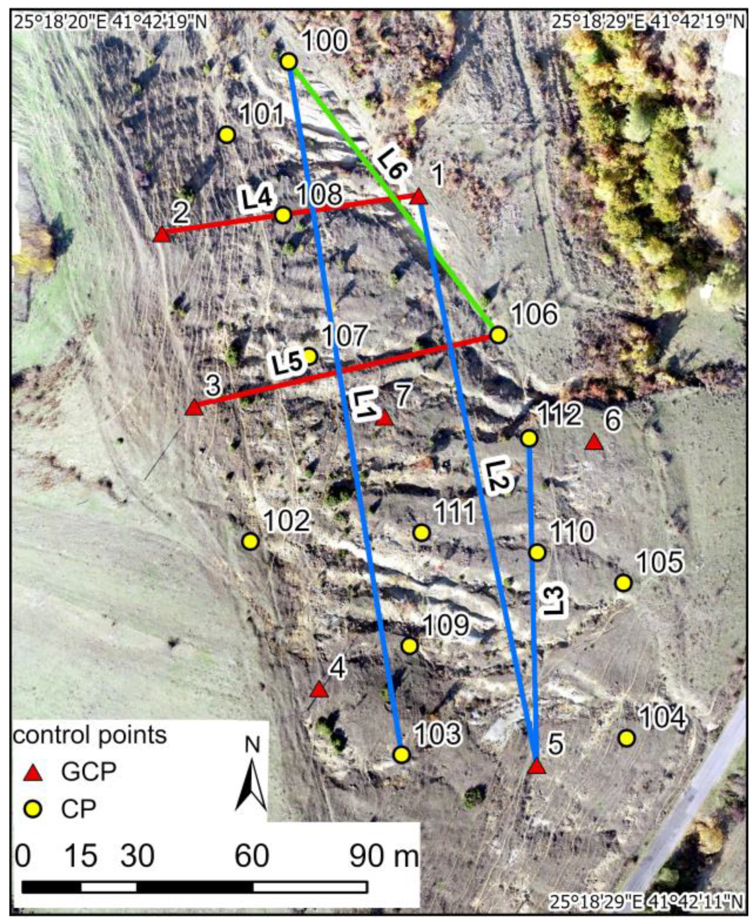
Three orthophotos were generated from the three image subcategories. A purely visual difference between them could not be seen as they look quite similar. For the purpose of the assessment, six lines were considered (Figure 8). They were selected regarding the morphometric features of the terrain. L1, L2, and L3 are located across the slope, perpendicular or nearly perpendicular to the line of maximal slope gradient. L4 and L5 are in the direction of the maximal slope gradient, and L6 follows nearly the gully bed in the lower part and cuts across the slope in the upper part. The differences between the lengths of these lines are determined by coordinate calculation and measured digitized lines are presented in Table 8.
In general, the differences are fairly small, which is associated with the high-accuracy and high-resolution products of UAS photogrammetry. Oblique imagery with a gimbal pitch angle at 60°—cross strips works better in measuring the length of L1, L2, and L6 where the percentage difference reached almost zero in three orthophotos of each subcategory. The differences between the length of reference lines L1, L2, and L3, and the corresponding three subcategories of lines are slightly larger than the corresponding differences for L4 and L5. This can be explained by the greater fragmentation of the relief in the cross-slope direction. In this case, oblique imagery (60°—cross strips mode) shows the best results, despite the fact that length differences in both other cases (nadir and 45° imagery) are also small.
Regarding the length of L4 and L5, which nearly follow the longitudinal slope profile, the results are very good using either nadir-viewing geometry. The differences in the length of the lines at the three subcategories compared to the reference line are negligible, except for L4, oblique imagery (45°—single strip). This can be explained by the relatively small length of the lines and the smaller variation of the terrain down the slope in comparison to the terrain variation in the direction across the slope. Similar results are presented by Kyriou et al. [18]. The authors state that nadir-viewing geometry gave the best results when the line intersects a smoother surface, while for a more complex profile line, a combination of nadir and oblique imagery shows better results in measuring the distances.
The difference in the measured distances in a gully longitudinal profile is insignificant (in a range of millimeters), in contrast to the measured distances in a direction across the slope, which reach up to 4–5 cm.
4. Discussion
Considering the point clouds, DSMs, and orthophotos, the results of the current study show that the differences in the properties of the photogrammetric products of 60°—cross strips oblique imagery and nadir—single strip mode are very small and can even be neglected. This can be explained by the features of the test area and the low vertical dissection of the relief. With regard to our results and the published materials on this topic, it can be concluded that in the delineating of small erosional landforms (rills, gullies) the flight geometry does not have a significant impact. However, the analysis of the differences in the length of the lines digitized on the orthophoto and reference length calculated by coordinates shows that oblique 60°—cross strips imagery is more reliable. The results of the study are in line with the findings of previous publications [18,20,22,38] that underline the advantage of the oblique imagery or a combination of nadir and oblique ones in the modelling of complex terrain. James and Robson [39] consider a single oblique camera angle as an option for reducing systematic deformation of the digital elevation model. According to Nesbit and Hugenholtz [22], supplementing nadir image blocks with oblique images in the UAV–SfM workflow consistently improves spatial accuracy. The tilt angle of the camera, combined with the slope of the terrain, has a significant impact on the detection of tie-points [40], which ensures the best fit of the images and impacts the quality of the results. Considering the DSM evaluations and differences in the values received from CutFill analysis, we can say that the flight geometry has a higher influence on volume calculation.
The spatial resolution of the photogrammetric products depends on the UAS flight parameters, characteristics of the images, camera parameters, and software capabilities. Śledź and Ewertowski [41] emphasize the level of accuracy set for dense point cloud generation. According to the cited authors, at the lowest level of processing, the resolution was ~28 cm, at the low level ~14 cm, at the medium level ~7 cm, at the high level ~3.5 cm, and at the ultra-high level ~1.75 cm. For the purpose of the current study, we performed the alignment of the images with a high-quality setting. At this option, the software works with photos of the original size [32]. Apart from the processing setting, the resolution of the derived models also depends on the camera tilt, if all other conditions are equal. In our study, we received at nadir-viewing imagery—3.5 cm; at oblique imagery 60°—cross strips—3.2 cm, and at oblique imagery 45°—single strip—4.5 cm for the pixel size. At the medium level of data processing, the results are, respectively: 7.0 cm -at nadir-viewing imagery and 9.7 cm—oblique imagery 45°—single strip. The above results direct attention to the parameters of photogrammetric processing and to the use of high or ultra-high levels of dense point cloud generation if the task concerns the evaluation of the geomorphic change due to slow geomorphological processes.
Regarding the evaluation of the DSMs and the computed vertical RMSE, the products based on the data of oblique imagery 60°—cross strips and nadir-viewing imagery are very similar; even the RMSE for the DSM derived from the nadir cloud is less compared to that of 60°—cross strips mode. Using GCPs significantly decreases high z errors for RTK surveys. Nota et al. [14] found that GCPs minimize the z errors to below 2 cm. The larger number of GCPs and their uniform distribution over the area can provide high-quality digital surface models, even with a medium option of the quality parameter of the photogrammetric processing [13]. GCPs are used not only for georeferencing but also for improving internal and external orientation parameters in photogrammetric processing [19]. In our study, we used a total of 20 points at a distance of about 20–30 m from each other and obtained GCPs and CPs RMSE around 2 cm and even less (Table 3).
According to Meinen and Robinson [42], the accuracy of nadir orientation images with a dense distribution of GCPs is comparable and quite close to that obtained from a terrestrial laser scanner. We can say that for a terrain with developed small erosional landforms and low values of vertical dissection of the relief, there are no significant differences between the DSMs of oblique imagery 60°—cross strips mode and nadir-viewing imagery, and the high number and density of the points in the clouds determine the small differences.
5. Conclusions
Based on the comparison of the point clouds, the lengths of the lines measured on the orthophoto mosaics, and the RMSE of the DSMs generated by the data of the three types of flight geometry used in the current study, the following conclusions can be drawn.
The M3C2 between the reference 60°—cross strip mode cloud and both compared clouds (nadir—single strip and 45°—single strip) shows small differences. The values near 0 are predominant. Closer are oblique 60°—cross strips and nadir—single strip imageries.
UAS camera tilt and plan geometry have a greater influence on volume calculation. To avoid over- and underestimation, RTK UAS is to be used with ground control points.
The comparison of the lengths of the lines digitized on the orthophotos against the reference line obtained from the X and Y coordinates shows larger differences in the case of the lines across the slope than of the lines drawn in the longitudinal direction of the slope (following the maximal slope gradient). In this particular study, oblique imagery 60°—cross strips mode shows greater accuracy. However, for this kind of erosional terrain, if the slope gradient is changing slowly, the nadir viewing geometry also produces good results.
In general, the comparisons of the photogrammetric products of the nadir single strip, oblique 45°—single strip, and oblique 60°—cross strips imagery reveal small differences that do not decisively determine the choice of the optimal UAS flight geometry in mapping small erosional landforms.
The small differences between the DSMs of the three flight geometries can be explained by the small size of the studied area, the large count of points in the clouds, and their high density. The results of the current study are closely related to the terrain features and the particular landscape conditions. Further studies of other areas with a relatively small vertical dissection of the relief are needed to evaluate the efficacy of the oblique geometry in studying erosional slopes, as well as to assess the transferability of the methodology.
Author Contributions
The authors contributed equally to elaborating the paper. Particular contributions are: conceptualization, V.N. and V.G.; methodology data acquisition, V.G. and A.K.; data processing and analyses, V.G., V.N. and A.K.; discussion and conclusion, V.N. and V.G., visualizations, V.N. All authors have read and agreed to the published version of the manuscript.
Funding
This research was carried out in the frame of the project “Application of geoinformation technologies in erosion research in mountain areas—Case studies of Eastern Rhodopes (Bulgaria)”, funded by the National Science Fund, Ministry of Education and Science (Bulgaria), Competition for financial support for basic research projects-2019 (Contract No KП-06-H34/3, signed on 5 December 2019).
Data Availability Statement
The data presented in this study are available on request from the corresponding author, upon reasonable request.
Acknowledgments
The authors thank the anonymous reviewers for their time and comments.
Conflicts of Interest
The authors declare no conflict of interest.
References
- Liu, W.-C.; Huanga, W.-C. Close range digital photogrammetry applied to topography and landslide measurements. Int. Arch. Photogramm. Remote Sens. Spat. Inf. Sci. 2016, 41, 875–880. [Google Scholar] [CrossRef]
- Mokhtar, M.R.M.; Wahab, S.N.A.; Bin, M.N.; Hashim, H.H.; Kasim, A.C. Landslide monitoring using close range photogrammetry. Plan. Malays. J. Malays. Inst. Plan. 2021, 19, 160–168. [Google Scholar] [CrossRef]
- Bazzoffi, P. Measurement of rill erosion through a new UAV-GIS methodology. Ital. J. Agron. 2015, 10 (Suppl. S1), 708. [Google Scholar] [CrossRef]
- Krenz, J.; Greenwood, P.; Kuhn, N.J. Soil degradation mapping in drylands using unmanned aerial vehicle (UAV) data. Soil Syst. 2019, 3, 33. [Google Scholar] [CrossRef]
- Liao, K.; Song, Y.; Xie, S.; Zheng, H. Monitoring of Benggang erosion based on UAV photogrammetry technology. IOP Conf. Ser. Earth Environ. Sci. 2019, 330, 052003. [Google Scholar] [CrossRef]
- Urban, R.; Štroner, M.; Blistan, P.; Kovanič, L.; Patera, M.; Jacko, S.; Ďuriška, I.; Kelemen, M.; Szabo, S. The suitability of UAS for mass movement monitoring caused by torrential rainfall—A study on the talus cones in the Alpine terrain in High Tatras, Slovakia. ISPRS Int. J. Geo.-Inf. 2019, 8, 317. [Google Scholar] [CrossRef]
- Ullman, S. The interpretation of structure from motion. Proc. R. Soc. Lond. 1979, 203, 405–426. [Google Scholar]
- Westoby, M.J.; Brasington, J.; Glasser, N.F.; Hambrey, M.J.; Reynolds, J.M. ‘Structure-from-motion’ photogrammetry: A low-cost, effective tool for geoscience applications. Geomorphology 2012, 179, 300–314. [Google Scholar] [CrossRef]
- Eltner, A.; Sofia, G. Structure from motion photogrammetric technique. Dev. Earth Surf. Process. 2020, 23, 1–24. [Google Scholar] [CrossRef]
- Rosas, M.A.; Clapuyt, F.; Viveen, W.; Vanacker, V. Quantifying geomorphic change in Andean river valleys using UAV-PPK-SfM techniques: An example from the western Peruvian Andes. Geomorphology 2023, 435, 108766. [Google Scholar] [CrossRef]
- Nikolakopoulos, K.G.; Kyriou, A.; Koukouvelas, I.K. Developing a Guideline of Unmanned Aerial Vehicle’s Acquisition Geometry for Landslide Mapping and Monitoring. Appl. Sci. 2022, 12, 4598. [Google Scholar] [CrossRef]
- James, M.R.; Robson, S.; D’Oleire-Oltmanns, S.; Niethammer, U. Optimising UAV Topographic Surveys Processed with Structurefrom-Motion: Ground Control Quality, Quantity and Bundle Adjustment. Geomorphology 2017, 280, 51–66. [Google Scholar] [CrossRef]
- Forlani, G.; Dall’Asta, E.; Diotri, F.; Cella, U.M.d.; Roncella, R.; Santise, M. Quality Assessment of DSMs Produced from UAV Flights Georeferenced with On-Board RTK Positioning. Remote Sens. 2018, 10, 311. [Google Scholar] [CrossRef]
- Nota, E.W.; Nijland, W.; De Haas, T. Improving UAV-SfM time-series accuracy by co-alignment and contributions of ground control or RTK positioning. Int. J. Appl. Earth Obs. Geoinf. 2022, 109, 102772. [Google Scholar] [CrossRef]
- Zimmerman, T.; Jansen, K.; Miller, J. Analysis of UAS Flight Altitude and Ground Control Point Parameters on DEM Accuracy along a Complex, Developed Coastline. Remote Sens. 2020, 12, 2305. [Google Scholar] [CrossRef]
- Lee, S.; Park, J.; Choi, E.; Kim, D. Factors Influencing the Accuracy of Shallow Snow Depth Measured Using UAV-based Photogrammetry. Remote Sens. 2021, 13, 828. [Google Scholar] [CrossRef]
- Seifert, E.; Seifert, S.; Vogt, H.; Drew, D.; Van Aardt, J.; Kunneke, A.; Seifert, T. Influence of Drone Altitude, Image Overlap, and Optical Sensor Resolution on Multi-view Reconstruction of Forest Images. Remote Sens. 2019, 11, 1252. [Google Scholar] [CrossRef]
- Kyriou, A.; Nikolakopoulos, K.; Koukouvelas, I. How image acquisition geometry of UAV campaigns affects the derived products and their accuracy in areas with complex geomorphology. ISPRS Int. J. Geo.-Inf. 2021, 10, 408. [Google Scholar] [CrossRef]
- Jiménez-Jiménez, S.I.; Ojeda-Bustamante, W.; de Jesús Marcial-Pablo, M.; Enciso, J. Digital Terrain Models Generated with Low-Cost UAV Photogrammetry: Methodology and Accuracy. ISPRS Int. J. Geo.-Inf. 2021, 10, 285. [Google Scholar] [CrossRef]
- Amrullah, C.; Suwardhi, D.; Meilano, I. Product accuracy effect of oblique and vertical non-metric digital camera utilization in UAV-photogrammetry to determine fault plane. ISPRS Ann. Photogramm. Remote Sens. Spat. Inf. Sci. 2016, III-6, 41–48. [Google Scholar] [CrossRef]
- Rossi, P.; Mancini, F.; Dubbini, M.; Mazzone, F.; Capra, A. Combining nadir and oblique UAV imagery to reconstruct quarry topography: Methodology and feasibility analysis. Eur. J. Remote Sens. 2017, 50, 211–221. [Google Scholar] [CrossRef]
- Nesbit, P.R.; Hugenholtz, C.H. Enhancing UAV–SfM 3D model accuracy in high-relief landscapes by incorporating oblique images. Remote Sens. 2019, 11, 239. [Google Scholar] [CrossRef]
- Nesbit, P.R.; Hubbard, S.M.; Hugenholtz, C.H. Direct Georeferencing UAV-SfM in High-Relief Topography: Accuracy Assessment and Alternative Ground Control Strategies along Steep Inaccessible Rock Slopes. Remote Sens. 2022, 14, 490. [Google Scholar] [CrossRef]
- Parmehr, E.G.; Savadkouhi, M.; Nopour, M. The impact of oblique images and flight-planning scenarios on the accuracy of UAV 3D mapping. Photogramm. Rec. 2023, 38, 563–580. [Google Scholar] [CrossRef]
- Lague, D.; Brodu, N.; Leroux, J. Accurate 3D comparison of complex topography with terrestrial laser scanner: Application to the Rangitikei canyon (N-Z). ISPRS J. Photogramm. Remote Sens. 2013, 82, 10–26. [Google Scholar] [CrossRef]
- Jordanov, B.; Sarov, S.; Georgiev, S.; Valkov, V.; Balkanska, E.; Grozdev, V.; Marinova, R.; Markov, N. Explanatory Note to Geological Map of Bulgaria, 1:50,000, Map Sheet K-35-75-G (Nikolovo); Ministry of Environment and Water, Bulgarian Geological Survey, Uniscorp Ltd.: Sofia, Bulgaria, 2008; p. 92. (In Bulgarian) [Google Scholar]
- DJI. Phantom 4 RTK User Manual, v.2.4. 2021. Available online: https://dl.djicdn.com/downloads/phantom_4_rtk/20210716/Phantom_4_RTK_User_Manual_v2.4_EN.pdf (accessed on 20 July 2023).
- Liu, Y.; Han, K.; Rasdorf, W. Assessment and Prediction of Impact of Flight Configuration Factors on UAS-Based Photogrammetric Survey Accuracy. Remote Sens. 2022, 14, 4119. [Google Scholar] [CrossRef]
- Haala, N.; Cramer, M.; Rothermel, M. Quality of 3D point clouds from highly overlapping UAV imagery. Int. Arch. Photogramm. Remote Sens. Spat. Inf. Sci. 2013, 40, 183–188. [Google Scholar] [CrossRef]
- Losè, T.L.; Chiabrando, F.; Tonolo, F.G. Boosting the timeliness of UAV large scale mapping. Direct georeferencing approaches: Operational strategies and best practices. ISPRS Int. J. Geo.-Inf. 2020, 9, 578. [Google Scholar] [CrossRef]
- Štroner, M.; Urban, R.; Seidl, J.; Reindl, T.; Brouček, J. Photogrammetry using UAV-mounted GNSS RTK: Georeferencing strategies without GCPs. Remote Sens. 2021, 13, 1336. [Google Scholar] [CrossRef]
- Agisoft LLC. Agisoft Metashape Professional. 2020. Available online: https://www.agisoft.com/pdf/metashape-pro_2_0_en.pdf (accessed on 1 December 2023).
- Özyeşil, O.; Voroninski, V.; Basri, R.; Singer, A. A survey of structure from motion. Acta Numer. 2017, 26, 305–364. [Google Scholar] [CrossRef]
- Lowe, D. Distinctive image features from scale-invariant keypoints. Int. J. Comput. Vis. 2004, 60, 91–110. [Google Scholar] [CrossRef]
- CloudCompare (Version 2.13 Beta) [GPL Software]. 2023. Available online: https://www.danielgm.net/cc/ (accessed on 28 November 2023).
- Zhang, W.; Qi, J.; Wan, P.; Wang, H.; Xie, D.; Wang, X.; Yan, G. An Easy-to-Use Airborne LiDAR Data Filtering Method Based on Cloth Simulation. Remote Sens. 2016, 8, 501. [Google Scholar] [CrossRef]
- ESRI Inc. ArcGIS Pro Software; version 3.2.1; ESRI Inc.: Redlands, CA, USA, 2023. [Google Scholar]
- Sammartano, G.; Chiabrando, F.; Spanò, A. Oblique images and direct photogrammetry with a fixed wing platform: First test and results in Hierapolis of Phrygia (TK). ISPRS Int. Arch. Photogramm. Remote Sens. Spat. Inf. Sci. 2020, 43, 75–82. [Google Scholar] [CrossRef]
- James, M.R.; Robson, S. Mitigating systematic error in topographic models derived from UAV and ground-based image networks. Earth Surf. Process. Landf. 2014, 39, 1413–1420. [Google Scholar] [CrossRef]
- Jaud, M.; Letortu, P.; Théry, C.; Grandjean, P.; Costa, S.; Maquaire, O.; Davidson, R.; Le Dantec, N. UAV survey of a coastal cliff face—Selection of the best imaging angle. Measurement 2019, 139, 10–20. [Google Scholar] [CrossRef]
- Śledź, S.; Ewertowski, M.W. Evaluation of the Influence of Processing Parameters in Structure-from-Motion Software on the Quality of Digital Elevation Models and Orthomosaics in the Context of Studies on Earth Surface Dynamics. Remote Sens. 2022, 14, 1312. [Google Scholar] [CrossRef]
- Meinen, B.U.; Robinson, D.T. Mapping erosion and deposition in an agricultural landscape: Optimization of UAV image acquisition schemes for SfM-MVS. Remote Sens. Environ. 2020, 239, 111666. [Google Scholar] [CrossRef]
Figure 1.
Study area: (a) geographical location; (b) orthophoto.

Figure 2.
UAS trajectories of data acquisition designed by DJI GS RTK app for Android, version: v. 2.2.5-GSP: (a) nadir—single strip with gimbal pitch angle at 90°; (b) oblique—single strip with gimbal pitch angle at 45°; (c) oblique—cross strip with gimbal pitch angle at 60°.
Figure 2.
UAS trajectories of data acquisition designed by DJI GS RTK app for Android, version: v. 2.2.5-GSP: (a) nadir—single strip with gimbal pitch angle at 90°; (b) oblique—single strip with gimbal pitch angle at 45°; (c) oblique—cross strip with gimbal pitch angle at 60°.
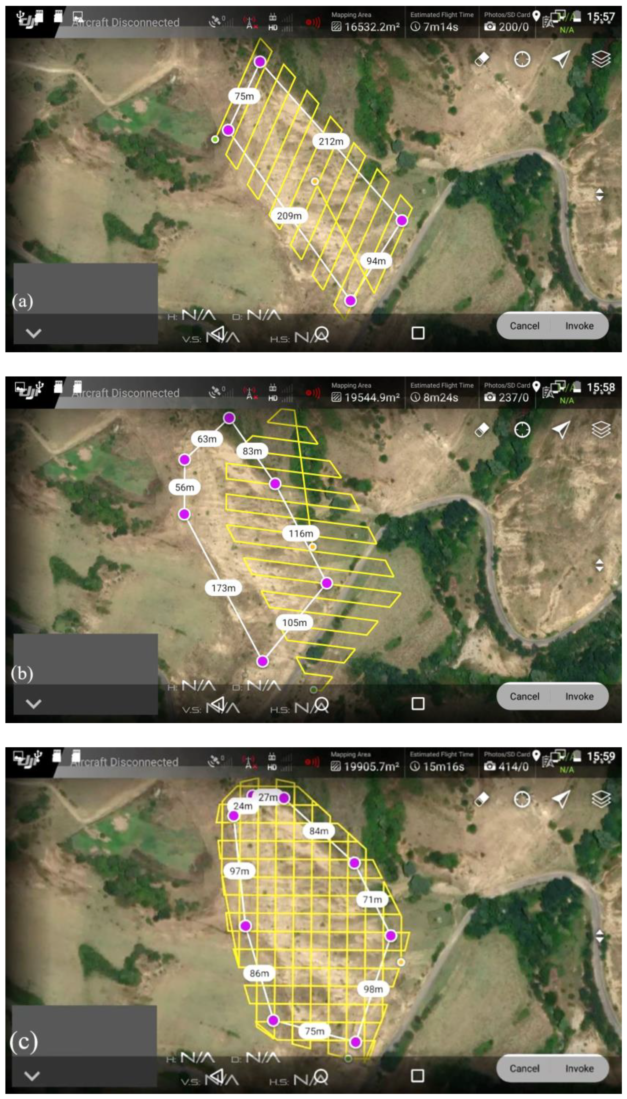
Figure 3.
Control points: (a) location of GCPs and CPs; (b) measurements of the points.
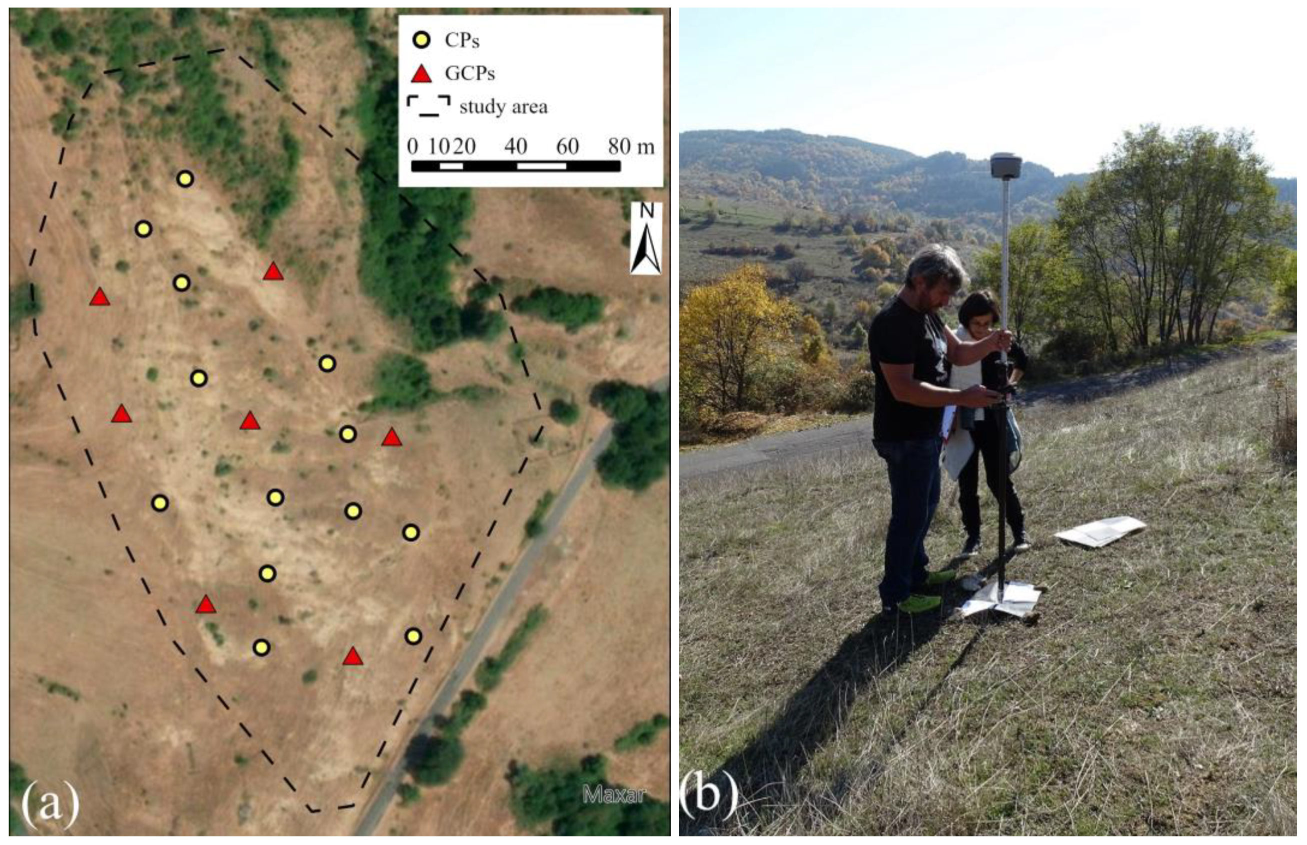
Figure 4.
Cloud to primitive entity comparison: (a) plan view; (b) profile view.

Figure 5.
Cloud to primitive distances in meters: (a) cloud of oblique 60°—cross strips mode to plane; (b) cloud of oblique 45°—single strip mode to plane; (c) cloud of nadir—single strip mode to plane.
Figure 5.
Cloud to primitive distances in meters: (a) cloud of oblique 60°—cross strips mode to plane; (b) cloud of oblique 45°—single strip mode to plane; (c) cloud of nadir—single strip mode to plane.
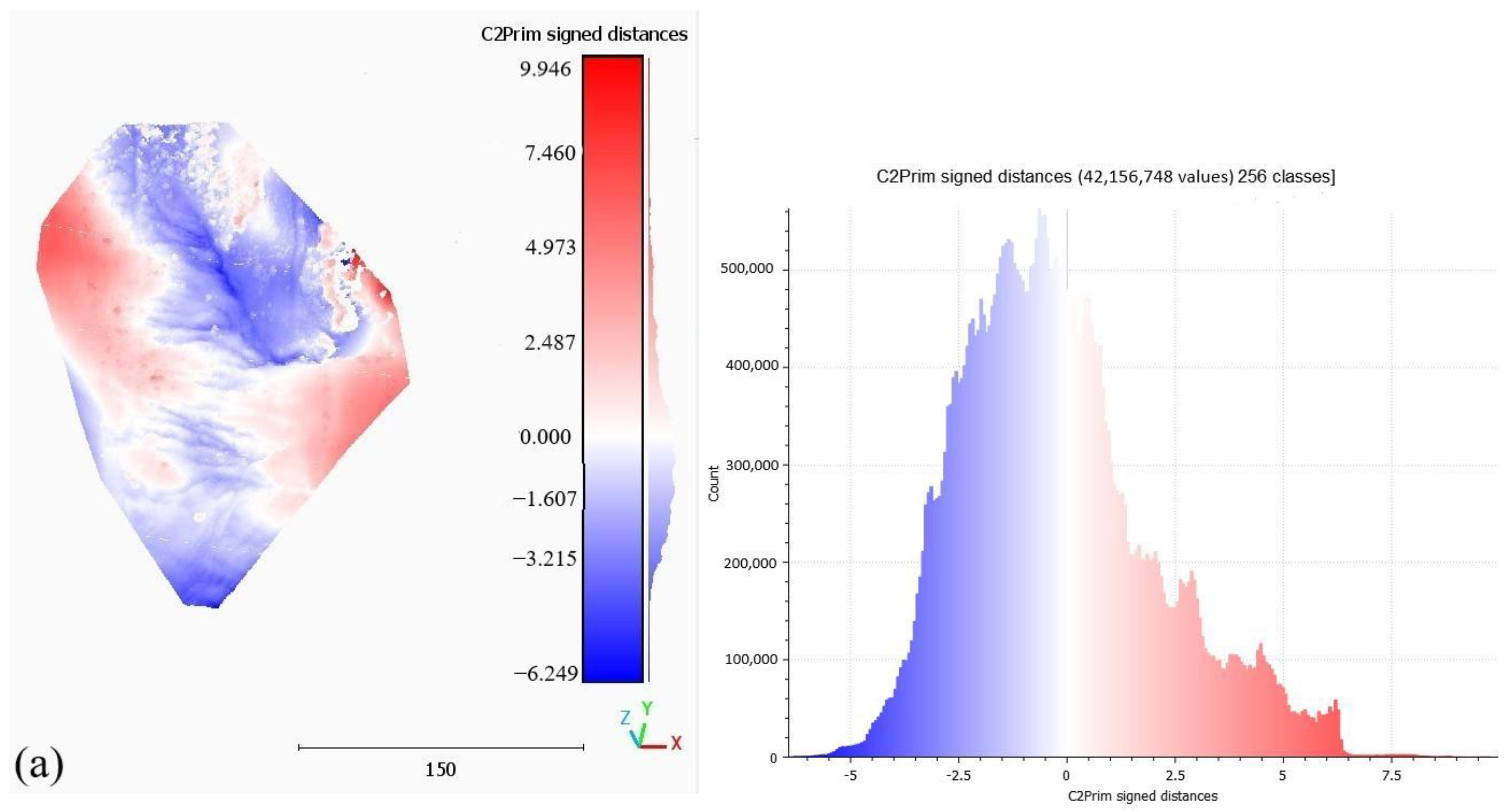

Figure 6.
M3C2 distances in meters computed between the reference point cloud of 60°—cross strips mode and: (a) nadir—single strip cloud; (b) cloud of 45°—single strip mode.
Figure 6.
M3C2 distances in meters computed between the reference point cloud of 60°—cross strips mode and: (a) nadir—single strip cloud; (b) cloud of 45°—single strip mode.

Figure 7.
Spatial distribution of the points in the clouds: (a) oblique imagery 45°—single strip mode; (b) oblique imagery 60°—cross strips mode; (c) nadir viewing imagery—single strip mode.
Figure 7.
Spatial distribution of the points in the clouds: (a) oblique imagery 45°—single strip mode; (b) oblique imagery 60°—cross strips mode; (c) nadir viewing imagery—single strip mode.

Figure 8.
Spatial distribution of the control points and the location of lines (L1–L6) throughout the study area (blue lines are across the line of maximal slope gradients; red lines are in the direction of maximal slope gradients, and the green line follows the gully cross-section in the upper part and nearly gully bed in the lower part).


Table 1.
Parameters of UAS flights.
| Indicator | Value |
|---|---|
| UAV altitude (m) | 60 |
| Ground sample distance (cm) | 1.67 ≈ 2 |
| Along the track overlap (%) | 80 |
| Across the track overlap (%) | 80 |
Table 2.
RTK GNSS observations of the ground points in WGS 84/UTM 35N (EPSG: 32635) spatial reference system (points from 1 to 7 are GCPs, and these from 100 to 112 are CPs).
Table 2.
RTK GNSS observations of the ground points in WGS 84/UTM 35N (EPSG: 32635) spatial reference system (points from 1 to 7 are GCPs, and these from 100 to 112 are CPs).
| Point | Northing | Easting | Height (m) | Hz. RMS (m) | Vert. RMS (m) | Satellites Used |
|---|---|---|---|---|---|---|
| 1 | 4618381.220 | 359135.010 | 613.960 | 0.018 | 0.026 | 31 |
| 2 | 4618371.366 | 359067.864 | 642.235 | 0.017 | 0.023 | 35 |
| 3 | 4618326.176 | 359076.314 | 637.090 | 0.018 | 0.024 | 35 |
| 4 | 4618252.511 | 359108.964 | 623.773 | 0.019 | 0.024 | 37 |
| 5 | 4618232.469 | 359165.857 | 605.703 | 0.018 | 0.025 | 34 |
| 6 | 4618317.131 | 359180.885 | 603.648 | 0.020 | 0.026 | 32 |
| 7 | 4618323.493 | 359126.056 | 619.714 | 0.020 | 0.027 | 31 |
| 100 | 4618416.033 | 359101.018 | 625.236 | 0.019 | 0.026 | 32 |
| 101 | 4618396.905 | 359084.878 | 631.483 | 0.019 | 0.026 | 32 |
| 102 | 4618290.638 | 359091.014 | 630.283 | 0.018 | 0.024 | 35 |
| 103 | 4618234.896 | 359130.596 | 616.081 | 0.018 | 0.024 | 36 |
| 104 | 4618239.270 | 359189.416 | 600.595 | 0.019 | 0.025 | 34 |
| 105 | 4618279.774 | 359188.594 | 601.805 | 0.019 | 0.026 | 35 |
| 106 | 4618344.579 | 359155.869 | 607.370 | 0.020 | 0.026 | 30 |
| 107 | 4618338.956 | 359106.313 | 623.936 | 0.021 | 0.027 | 32 |
| 108 | 4618375.844 | 359099.596 | 628.198 | 0.021 | 0.028 | 32 |
| 109 | 4618263.361 | 359132.658 | 615.944 | 0.019 | 0.025 | 35 |
| 110 | 4618287.738 | 359166.025 | 608.150 | 0.020 | 0.025 | 35 |
| 111 | 4618292.918 | 359135.854 | 615.921 | 0.020 | 0.027 | 36 |
| 112 | 4618317.514 | 359163.893 | 607.896 | 0.019 | 0.025 | 30 |
Table 3.
Camera location errors and RMSE at the different flight plans, according to the SfM Agisoft report.
Table 3.
Camera location errors and RMSE at the different flight plans, according to the SfM Agisoft report.
| Capture Type | Average Camera Location Error Total Error (cm) | RMSE (m) GCPs | RMSE (m) CPs |
|---|---|---|---|
| Nadir—single strip | 1.5 | 0.020 | 0.025 |
| Oblique—single strip with gimbal pitch angle at 45° | 1.7 | 0.014 | 0.021 |
| Oblique—cross strip with gimbal pitch angle at 60° | 1.8 | 0.007 | 0.013 |
Table 4.
Distribution of positive and negative values of cloud to primitive distances (% of the total cases).
Table 4.
Distribution of positive and negative values of cloud to primitive distances (% of the total cases).
| Oblique Imagery 60°— Cross Strips | Oblique Imagery 45°— Single Strip | Nadir Imagery 90°— Single Strip | |||
|---|---|---|---|---|---|
| Positive Values | Negative Values | Positive Values | Negative Values | Positive Values | Negative Values |
| 40.99 | 59.01 | 41.91 | 58.09 | 40.96 | 59.04 |
Table 5.
Point counts per m2. (ArcGIS Pro statistics of rasters whose cell values reflect statistical information about LAS points).
Table 5.
Point counts per m2. (ArcGIS Pro statistics of rasters whose cell values reflect statistical information about LAS points).
| Capture Type | Mean | Maximum | Minimum |
|---|---|---|---|
| Oblique imagery 45°—single strip | 510 | 1483 | 1 |
| Oblique imagery 60°—cross strips | 1183 | 3460 | 1 |
| Nadir imagery—single strip | 965 | 2858 | 1 |
Table 6.
Vertical RMSE (m) of the DSMs, generated from the clouds according to the respective control points.
Table 6.
Vertical RMSE (m) of the DSMs, generated from the clouds according to the respective control points.
| Point Cloud for the Creation of the DSM | |||
|---|---|---|---|
| DSM | 60°—Cross Strips | 45°—Single Strip | Nadir—Single Strip |
| DSM—automatically generated in Agisoft in cloud processing | 0.024 (DSM cell size 0.032 m) | 0.040 (DSM cell size 0.049 m) | 0.022 (DSM cell size 0.35 m) |
| DSM—cell size 0.05 m | 0.024 | 0.037 | 0.022 |
| DSM—cell size 0.10 m | 0.023 | 0.037 | 0.022 |
Table 7.
CutFill comparison with a theoretical plane, volumes in m3.
| 60°—Cross Strips Mode Cloud | 45°—Single Strip Mode Cloud | Nadir—Single Strip Mode Cloud | |||
|---|---|---|---|---|---|
| Above the surface | 31,389.58 | 32,255.84 | 31,462.17 | ||
| Below the surface | 35,194.55 | 34,027.38 | 35,083.88 | ||
| Difference: between 60° and 45° clouds | above the surface | below the surface | |||
| −866.26 | 1167.16 | ||||
| Difference: between 60° and 90° clouds | above the surface | below the surface | |||
| −72.59 | 110.67 | ||||
Table 8.
Lengths of the reference lines and the corresponding digitized lines (the number of lines corresponds to the one given in Figure 8).
Table 8.
Lengths of the reference lines and the corresponding digitized lines (the number of lines corresponds to the one given in Figure 8).
| UAS Data | Distance, m | Difference with the Reference Line, m * | Difference, % |
|---|---|---|---|
| Line 1 (L1) | |||
| Reference lines from X and Y coordinates | 183.536 | ||
| Nadir imagery (90°—single strip) | 183.582 | −0.046 | −0.03 |
| Oblique imagery (45°—single strip) | 183.585 | −0.049 | −0.03 |
| Oblique imagery (60°—cross strips) | 183.580 | −0.044 | −0.02 |
| Line 2 (L2) | |||
| Reference lines from X and Y coordinates | 151.916 | ||
| Nadir imagery (90°—single strip) | 151.951 | −0.035 | −0.02 |
| Oblique imagery (45°—single strip) | 151.937 | −0.021 | −0.01 |
| Oblique imagery (60°—cross strips) | 151.936 | −0.020 | −0.01 |
| Line 3 (L3) | |||
| Reference lines from X and Y coordinates | 85.068 | ||
| Nadir imagery (90°—single strip) | 85.118 | −0.05 | −0.06 |
| Oblique imagery (45°—single strip) | 85.111 | −0.043 | −0.05 |
| Oblique imagery (60°—cross strips) | 85.107 | −0.039 | −0.05 |
| Line 4 (L4) | |||
| Reference lines from X and Y coordinates | 67.865 | ||
| Nadir imagery (90°—single strip) | 67.867 | −0.002 | 0.00 |
| Oblique imagery (45°—single strip) | 67.921 | −0.056 | −0.08 |
| Oblique imagery (60°—cross strips) | 67.881 | −0.016 | −0.02 |
| Line 5 (L5) | |||
| Reference lines from X and Y coordinates | 81.656 | ||
| Nadir imagery (90°—single strip) | 81.660 | −0.004 | −0.01 |
| Oblique imagery (45°—single strip) | 81.658 | −0.002 | 0.00 |
| Oblique imagery (60°—cross strips) | 81.661 | −0.005 | −0.01 |
| Line 6 (L6) | |||
| Reference lines from X and Y coordinates | 90.080 | ||
| Nadir imagery (90°—single strip) | 90.099 | −0.019 | −0.02 |
| Oblique imagery (45°—single strip) | 90.069 | 0.011 | 0.01 |
| Oblique imagery (60°—cross strips) | 90.083 | −0.003 | 0.00 |
* the smallest differences are presented in bold.
Disclaimer/Publisher’s Note: The statements, opinions and data contained in all publications are solely those of the individual author(s) and contributor(s) and not of MDPI and/or the editor(s). MDPI and/or the editor(s) disclaim responsibility for any injury to people or property resulting from any ideas, methods, instructions or products referred to in the content. |
© 2024 by the authors. Licensee MDPI, Basel, Switzerland. This article is an open access article distributed under the terms and conditions of the Creative Commons Attribution (CC BY) license (https://creativecommons.org/licenses/by/4.0/).
Share and Cite
MDPI and ACS Style
Nikolova, V.; Gospodinova, V.; Kamburov, A. Assessment of Unmanned Aerial System Flight Plans for Data Acquisition from Erosional Terrain. Geosciences 2024, 14, 75. https://doi.org/10.3390/geosciences14030075
AMA Style
Nikolova V, Gospodinova V, Kamburov A. Assessment of Unmanned Aerial System Flight Plans for Data Acquisition from Erosional Terrain. Geosciences. 2024; 14(3):75. https://doi.org/10.3390/geosciences14030075
Chicago/Turabian StyleNikolova, Valentina, Veselina Gospodinova, and Asparuh Kamburov. 2024. "Assessment of Unmanned Aerial System Flight Plans for Data Acquisition from Erosional Terrain" Geosciences 14, no. 3: 75. https://doi.org/10.3390/geosciences14030075
Note that from the first issue of 2016, this journal uses article numbers instead of page numbers. See further details here.