

Assessments of Gravity Data Gridding Using Various Interpolation Approaches for High-Resolution Geoid Computations


Gravity Research Group, Geomatics Engineering Department, Istanbul Technical University, Istanbul 34469, Turkey
*
Author to whom correspondence should be addressed.
Geosciences 2024, 14(3), 85; https://doi.org/10.3390/geosciences14030085
Submission received: 29 December 2023
/
Revised: 14 March 2024
/
Accepted: 15 March 2024
/
Published: 19 March 2024
(This article belongs to the Special Issue Earth Observation by GNSS and GIS Techniques)
Abstract
:This article investigates the role of different approaches and interpolation methods in gridding terrestrial gravity anomalies. In this regard, first of all, simple and complete Bouguer anomalies are considered in gravity data gridding. In the comparison results of gridding these two Bouguer anomaly datasets, the effect of the high-frequency contribution of topographic gravitation (by means of the terrain correction) is clarified. After that, the role of the used interpolation algorithm on the resulting grid of mean gravity anomalies and hence on the geoid modeling accuracy is inspected. For this purpose, four different interpolation methods including geostatistical Kriging, nearest neighbor, inverse distance to a power (IDP), and artificial neural networks (ANNs) are applied. Here, the IDP and nearest neighbor methods represent simple-structured algorithms among the interpolation methods tested in this study. The ANN method, on the other hand, is preferred as a complex, optimization-based soft computing method that has been applied in recent years. In addition, the geostatistical Kriging method is one of the conventional methods that is mostly applied for gridding gravity data in geodesy and geophysics. The calculated gravity anomalies in grids are employed in high-resolution geoid model computations using the least squares modifications of Stokes formula with additive corrections (LSMSA) technique. The investigations are carried out using the test datasets of Auvergne, France that are provided by the International Service for the Geoid for scientific research. It is concluded that the interpolation algorithms affect the gravity gridding results and hence the geoid model determination. The ANN method does not provide superior results compared to the conventional algorithms in gravity gridding. The geoid model with 4.1 cm accuracy is computed in the test area.
1. Introduction
In many applications of geodesy, geophysics, geodynamics, and engineering disciplines, the height information of a point relative to a reference surface is essential. Ellipsoidal height, which is the vertical distance between a point on the Earth’s surface and an ellipsoid along the ellipsoidal normal, can be obtained anywhere and anytime, regardless of weather conditions, using global navigation satellite systems (GNSS). However, this kind of height cannot be utilized for the majority of engineering and surveying applications, including drainage projects, building engineering structures, managing natural disasters, etc., as it only has geometrical meaning and does not refer to the Earth’s gravitational field [1,2,3]. Instead, the orthometric height is utilized, which indicates a natural flow of the fluids, as it refers to the Earth’s gravitational field and is described as the distance between the geoid and a point on the Earth’s surface [4,5,6]. Leveling is the conventional measurement technique for precise determination of the orthometric heights. However, this method is a time-consuming and expensive task in practice. In addition, it is prone to error accumulation, especially in large areas, and is more difficult to carry out in rough terrain. Deformations, especially occurring in active tectonic regions, require updating the vertical control networks that rely on leveling measurements, which is a significant disadvantage for vertical control networks. Therefore, acquiring the orthometric height () of a topography point using its GNSS-ellipsoidal height () and geoid height (), which is the distance between the geoid and ellipsoid along the ellipsoid normal at the point (), is an efficient method in surveying applications. In this method, the geoid height parameter is obtained using a geoid model, and the accuracy of the orthometric height in this transformation is directly related to the accuracy of the geoid model. In order to obtain the orthometric heights within a few centimeters of accuracy, high-resolution regional geoid models determined using dense and accurate terrestrial gravity data are used [5,7,8,9].
The geoid is a level surface with a constant gravity potential, and it coincides with the mean sea level after removing the effects of sea surface topography over the oceans [10]. The determination of the geoid surface relies on a boundary value problem solution represented by the Stokes formula and adopts an assumption of no masses outside of the geoid surface. In order to fulfill this condition, the topographical masses outside of the geoid are mathematically excluded in geoid computation theory. The implementation of the Stokes formula requires a global coverage of terrestrial gravity observations, but having dense terrestrial gravity observations over the entire Earth is not practically possible. The consequence of this data deficiency in the results is minimized by integrating locally available dense terrestrial gravity data and globally available satellite gravity observations in a modified Stokes integral formula. A stochastic modification of the Stokes integral formula is utilized in the least squares modification of Stokes integral with additive corrections (LSMSA) approach developed by the Royal Institute of Technology in Sweden (or shortly the KTH approach). This approach has been used in the determination of the regional geoid models in many studies so far, and it has yield accurate results in these studies (see [3,7,11,12,13,14,15,16,17,18,19,20,21,22,23,24,25,26,27,28,29,30,31]). In addition to the KTH method, there are also different gravimetric geoid determination algorithms used for regional gravimetric geoid modeling in the literature (see [32,33,34,35,36,37]).
In geoid model computations using the LSMSA method, the free air gravity anomalies in the grid form on the surface of the topography are used. These free air anomalies are restored from gridded Bouguer anomalies on the geoid. For gridding terrestrial gravity data, observed gravity values () are transformed into gravity anomalies () and are reduced to the reference surface “geoid” using the Bouguer reduction procedure. In the reduction of gravity anomalies, the gravitational attraction effects caused by topographic masses above the geoid are simply calculated and removed from gravity observations [38,39]. According to implemented reduction components, either simple or complete (refined) Bouguer gravity anomalies can be calculated and applied. In simple Bouguer reduction, the topography is identified just as the Bouguer plate (or shell), and the masses described by this plate above the geoid are removed. Even though the simple Bouguer anomalies (SBAs) do not include the effects of residual topographical masses deviating from the plate, complete Bouguer anomalies consider these excess terrain effects. Thus, the CBAs are acquired by adding the terrain corrections (TC) to the simple Bouguer anomalies. Simple or complete Bouguer gravity anomalies are preferred to be used for gravity data interpolation and gridding due to their low-frequency characteristics with less dependency on topographic variations [40,41]. Several studies have investigated whether SBAs may be utilized in gravity data interpolation and gridding instead of CBAs. While free-air anomalies (FAAs) are affected by the aliasing effect more than simple Bouguer anomalies, complete Bouguer anomalies are smoother and less sensitive to the negative effects of aliasing than both anomalies, in theory. According to Abbak et al. [38], Goos and Featherstone [42], and Kuhn et al. [43], the use of CBAs is crucial when topography is rough due to extreme elevation variations, but SBAs can also be used in smooth regions despite the omission of the high-frequency effect of residual topographical masses. Carrying out data gridding using appropriate types of gravity anomalies is crucial for the geoid determination. Inappropriately gridded gravity dataset may lead to a loss of the gravity signal in the input data and hence reduce the quality of the preformed regional geoid model. As stated above, removing high-frequency information obtained via terrain corrections prior to the gridding can solve the aliasing problem in the input gravity grid data. On another hand, densifying the gravity observations can also minimize this error, but this option may not always be possible, especially in rough topographies and restricted observational areas for. Digital elevation model (DEM) data are used for calculating the gravitational effects of topographic masses in Bouguer reduction process [2,41,44]. Also, the geoid computation using the LSMSA method employs DEM for calculating the terrain and downward continuation (DWC) corrections, which are restored onto the approximate geoid height parameter obtained from a global geopotential model (GGM) as the low-frequency component of the geoid [44].
This research is carried out using gravity observations in the Auvergne test area in France. It aims to investigate the role of interpolation methods in gridding the terrestrial gravity anomalies and their consequences on geoid model determination. Within the scope of the study, firstly, we test and clarify the role of the used Bouguer gravity anomaly type in the gridding process and hence its consequence on the geoid model determination. For this purpose, we grid the simple (SBAs) and complete (CBAs) Bouguer anomalies, employing the geostatistical Kriging interpolation algorithm, which is a commonly used technique in gravity field determination studies. Since the LSMSA method uses free air anomalies on the Earth’s surface, free air anomalies in grid form are obtained by applying the Bouguer plate and terrain correction values to the gridded Bouguer anomalies [7]. The statistics obtained from the areal comparison of the SBA and CBA grids at grid nodes and validations of the geoid models in the study area are used to clarify the significance of the Bouguer anomaly type in the data gridding process.
Secondly, the effects of the interpolation techniques used in gridding the CBAs on geoid determination are investigated in this study. Four interpolation algorithms (Kriging, inverse distance to a power (IDP), nearest neighbor, and artificial neural network (ANN) methods) are employed. Here, it is worth emphasizing that this investigation does not aim to find the best interpolator but rather to clarify the role of employing a different interpolator in gravity gridding. Among these methods, ordinary Kriging is one of the most common two methods (the other is the Least Squares Collocation method) used in gravity field and geoid modeling studies. These methods are generally employed in data interpolation modules of the geoid computation software suits as in the KTH-Geolab software for precise geoid determination [18,19,20], as well as GRAVSOFT geodetic gravity field modeling programs [28,35,36]. The IDP and nearest neighbor algorithms are two widely used interpolation methods not only in the field of gravity research but also in various application areas where spatial data interpolation is required. Both algorithms dominate the local characteristics in the interpolation results via weighting the data or limiting the interpolation boundaries. Additionally, the simplicity of their formulations is an advantage for these two algorithms from a computational practicality point of view. In addition to these three widely used interpolation methods, we also apply an artificial neural network for gridding the complete Bouguer anomalies as the fourth method in this study. The ANN is a learning-based soft computing algorithm, and due to this aspect, it is quite different from the other three algorithms tested here. We included the ANN in this study to verify the performance of a recent generation interpolation algorithm in gravity gridding and to compare it with the widely used conventional techniques. Subsequently, new geoid models are acquired using free air anomaly grid datasets. A comparison of the calculated geoid models at the grid nodes provides the areal differences among the models. The validation of the geoid models using the GPS/leveling benchmarks in the area reveals an absolute accuracy value for the calculated geoid models.
The conclusions drawn from this investigation indicate that in regions with plain topography, since the terrain correction parameters remain within certain limits, either simple or complete Bouguer gravity anomalies can be used in gravity gridding. However, in rough terrain, the differences between simple and complete Bouguer anomalies are considerable; therefore, complete Bouguer anomalies should be used. In gravity gridding, the used interpolation algorithm affects both the magnitude and distribution pattern of the gravity values at the grid nodes and influences the geoid model computations. Using the conventional interpolation algorithms (Kriging, the IDP, and the nearest neighbor), the gravity value at a grid node is estimated directly using the data at the observation points, and the contribution of the data point is formulated in the algorithm. The Kriging method also takes the stochastic properties of the observations, employing covariances in its algorithm. Since they have similarities in their mathematical backgrounds, their output grids have smaller differences in magnitude. Contrary to expectations, the ANN, a learning-based soft computing method, does not provide superiority over the conventional methods in this study. As a result of the tests, the grid datasets obtained using the Kriging, IDP and nearest neighbor interpolation algorithms were found to be the most compatible. As a result of the calculations, the accuracy of the geoid models computed in the region is 4.1 cm.
2. Materials and Methods
Basic definitions and formulas of gravity anomalies and terrain reductions are given here within the context of gravimetric geoid computations. Then interpolation techniques, which play an important part in the gridding procedure for Bouguer anomalies, are discussed. Thereafter, least squares modifications of Stokes formula with additive corrections (LSMSA) method is expressed using detailed formulas.
2.1. Gravity Anomalies and Terrain Correction
The observed gravity values on the topography are not suitable for interpolation since they contain high-frequency components of Earth’s gravitational field. Thus, randomly distributed gravity data on topography has to be reduced to the geoid surface for the purposes of geoid determination, interpolation, and extrapolation of gravity data and geophysical exploration studies. The geoid can be computed using Stokes integral and gravity anomalies on the geoid are its input data in computations. The geoid height parameter () is the output in this computation [7,24,38,44,45]. In other words, surface gravity anomalies have to be downward continued to the geoid surface using a suitable reduction schema before the geoid computation. The difference between the gravity value at a point on the geoid surface () and the normal gravity at its corresponding point on the ellipsoid () is described as the gravity anomaly on the geoid (); see Equation (1) below [10,39,41]:
The need for reductions in gravity anomalies to the geoid stems from the requirement of regular grid usage of geoid computation algorithms such as the LSMSA method. Therefore, pointwise gravity anomalies on the Earth’s surface are transformed into simple or complete (refined) Bouguer anomalies that have smooth characteristics for interpolation processes [11,13]. Although the interpolation process directly affects the accuracy of the geoid computation, the choice of the optimum interpolation techniques plays an important role [7,46].
In geodesy, Bouguer anomalies are important to use for gridding process and data interpolation purpose [11,13]. These anomalies are also necessary because many geoid modeling algorithms evaluate the gravity data in grid form. Additionally, Bouguer anomalies are also used to explain geological structures in geophysics disciplines [43]. In Bouguer reduction, the topography is represented as plate (or shell), and the gravitation of all the masses within this plate above the geoid are calculated and removed from the observed gravity. Here, the thickness of the Bouguer plate is , and it is equal to the height of topographic point P [40,41]. An illustration of a Bouguer plate is given in Figure 1 below [10,47]:
Simple Bouguer anomalies () can be computed as shown in Equation (2) [39,44]:
where is the observed gravity at point having orthometric height , is the normal gravity value calculated at point on the ellipsoid surface, is the Bouguer plate reduction parameter, and is the free air reduction parameter. The planar Bouguer reduction parameter is given in Equation (3):
where is the gravitational constant ( = 6.672585 × 10⁻¹¹ m3 kg−1 s−2) and is the topographical mass density. In the computations, the mass density is generally assumed to be constant as = 2670 kg m−3. Hence, after substituting the constants into the above formula, it is rewritten as in Equation (4):
in the equation, is in mGal and is in meters. The free air correction that takes the observed gravity in free air down to the geoid using the vertical gradient of the gravity is formulated as in Equation (5) [5,41]. However, in the equation, there is an assumption because the normal gradient of gravity (associated with the ellipsoidal height ) is used instead of . But, in Hofmann-Wellenhof and Moritz [5], it is confirmed that this equation can be used, and it gives sufficient precision for many practical applications (see p. 134 in [5]).
Complete Bouguer anomalies () are calculated by adding another correction term named terrain correction () to simple Bouguer anomalies, which removes the gravitational effect of residual topographical masses deviating from the Bouguer plate (see Figure 1), as formulated in Equation (6) [39,47]:
In Equation (6), is the free air anomalies and is expressed as in Equation (7):
The summation of the Bouguer reduction () and terrain correction () parameters is called terrain reduction.
The normal gravity () computed on the reference ellipsoid is calculated using Somigliana formula in Equation (8) [8,43]:
where is geocentric latitude, is the normal gravity at the equator (), is the normal gravity constant, and the eccentricity is formulated as , where and are the semi-major and semi-minor axes of the reference ellipsoid, respectively. The GRS80 (Geodetic Reference System 1980) ellipsoid parameters are used in this study for the computation of normal gravity; see Table 1 for the parameters [48]:
The formula of terrain correction () is given in Equation (9) [2,49]:
where is the topographic height at the computation point, corresponds to the height of the running point, is the integration area, and is the density of the topographical masses. The distance between the computation point and the running point can be calculated as shown in Equation (10):
In this study, terrain corrections are computed using the TC module of the GRAVSOFT geodetic gravity field computation software [50,51], and the geoid models are calculated using the ITU-LSMSA geoid computation software produced by Istanbul Technical University Gravity Research Group (ITU-GRG).
We utilize the planar Bouguer reduction formulas in the tests since the computation area has a reasonable size and planar approach, satisfying the objectives in this research. However, instead of a planar approach, the gravitation of the topographic masses can also be formulated in a spherical approximation using Bouguer reduction. The Bouguer shell correction () in the spherical approach is formulated as shown in Equation (11):
The terrain corrections in the spherical Bouguer reduction are calculated using global topography data, which is a significant burden. Detailed formulation of the spherical Bouguer reduction schema can be found in Kuhn et al. [43]. Comparative results of planar and spherical approaches in the Bouguer reduction with discussions are given in Abbak et al. [38], Vanicek et al. [52,53], Erol et al. [54], Hackney and Featherstone [8], and Tziavos and Sideris [41].
Digital elevation model (DEM) data is used in terrain reduction. The height information used in the computation of the Bouguer plate correction and terrain correction parameters are obtained from a high-resolution digital elevation model of the study area. Hence, the resolution and accuracy of the used DEM data affect the accuracy of the gridding process [40,41,42,55]. In addition, the DEM data are used in the computation of the downward continuation effect in geoid modeling using the LSMSA method (see in Section 2.3) [44,56]. In this study, we use high-resolution global shuttle radar topography mission (SRTM) digital elevation model data with 3 arc-second spatial resolution [57]. The SRTM DEM data are freely available from U. S. Geological Survey [58]. The horizontal position of the DEM grids is in the WGS84 datum, and its height data bases are on the EGM96 global geoid surface. The vertical accuracy of the SRTM3 DEM data is reported as ~9 m over the Earth [57,58]. This accuracy is confirmed with the local validation results from different countries such as the Himalayan site of India [59], Croatia [60], and Turkey [61].
2.2. Interpolation Algorithms
As stated in the previous sections, Bouguer anomalies are employed in the gridding process due to their smooth features, whereas free air anomalies have a higher correlation with the topographical changes [39]. For the gridding process of simple or complete Bouguer anomalies, interpolation algorithms including geostatistical Kriging, inverse distance to a power (IDP—also called IDW), nearest neighbor, and artificial neural network (ANNs) are carried out in this study [62,63]. Thus, the basic characteristics of these methods are described here [64,65].
2.2.1. Nearest Neighbor
The nearest neighbor interpolation algorithm (also known as point-sampling in some cases) is quite simple to implement and is commonly used in spatial data gridding problems. Rather than calculating an average value based on some weighting criteria as in the IDP method, this algorithm selects the value of the nearest point and does not consider the values of the other neighboring points. In data gridding using the nearest neighbor method, the nearest data point to the grid node to be estimated is searched for and used [66,67,68].
2.2.2. Inverse Distance to a Power (IDP)
This deterministic method is based on a weighted average of the observed values (data points) considering the closeness. The observations closer to the points to be interpolated have higher weights. This method is very fast and useful when the observed values are distributed irregularly or sparse; however, the formation of bull’s eye can occur [63,69]. Modifying the smoothing parameter can resolve this problem. IDP can be formulated as shown in Equations (12) and (13) [66,70]:
where is the interpolated data, is the observed data, is the weight of , is the number of observations, is the distance between the interpolated and observed value, is the effective separation distance between the interpolated point () and the observed point (), is the smoothing parameter, and is the power parameter ( = 1, 2 or 3).
The power parameter controls how fast the weights decrease as they approach the interpolated value. In other words, the influence of locations far from the estimation points during interpolation decreases with increasing weighting power. Usually, the power parameters are chosen within a range of one to three [63,71]. In our study, the power parameter is chosen as 2. The uncertainty factor can be applied to sample data using the smooth option on the software. By increasing the smoothing parameter, the effects of specific observations on gridding process can be decreased [66].
2.2.3. Kriging
This commonly used geostatistical gridding method, which can be exact or smooth, is based on spatial variance as a distance-dependent function and is applicable to all kinds of datasets. In contrast to IDP and nearest neighbor, Kriging has the slowest computation speed and performs with a smoother display [66,71].
The observed point’s spatial continuity or roughness can be described using the variogram. There are numerous variogram models on the Surfer that identify the spatial relationship mathematically, such as exponential, Gaussian, linear, logarithmic, nugget effect, power, quadratic, rational quadratic, spherical, wave, cubic, and penta-spherical. The choice of the drift type identifies the discrimination of ordinary and universal Kriging. If the drift type is chosen as linear or quadratic, the Kriging is termed universal. Otherwise, no drift indicates an ordinary Kriging that presumes a constant unknown mean over the specified area [66].
Another separation can be practiced as point and block Kriging that are applicable to both ordinary and universal Kriging approaches. The points at the grid nodes are calculated using point Kriging, whereas the averages of the blocks are computed using block Kriging by using blocks that are centered on the nodes [65,66,72]. The basic equation of ordinary Kriging is as follows [73,74]:
where is the weight, is the observed data, and is the interpolated data. In the computations, we use ordinary Kriging with a linear variogram model. The Kriging type is the point Kriging.
2.2.4. Artificial Neural Network (ANN)
The artificial neural network (ANN) is a widely used soft computing algorithm that was designed by imitating the human nervous system. The algorithm can be trained using sample data and estimates the target value using network connections based on weights.
The algorithm can be used in many fields such as the automotive industry, banking, amusement sector, aerospace, and so on. Moreover, it can also be used for the calculation of geodetic deformations, prediction of sea level changes, and estimation of the orientation parameters of Earth [75,76,77,78,79,80].
The algorithm runs with the “nnstart” command on MATLAB, and “nntool” is not available for versions later than R2022a [81]. There are various ANN techniques built into the MATLAB software such as radial basis, generalized regression, NARX, hopfield, feed-forward backpropagation, Elman backpropagation, etc. [75,82,83]. Here, the feed-forward backpropagation technique is used with the “trainlm” function, which specifies the Levenberg–Marquardt approach. Additionally, the “tansig” transfer function and “learngdm” adaption learning function with 2 layers and 200 neurons are chosen to specialize the method (see Figure 2). In contrast to the Levenberg–Marquardt approach, which is fast but requires a high memory capacity, there are also two other common methods named Bayesian regularization (trainbr) and scaled conjugate gradient (trainscg). See Demuth et al. [75] for further information.
The network geometry of feed-forward backpropagation consists of neurons within parallel layers that are classed as input, hidden, and output layers. The data are presented to the network via the input layer, whereas the desired output values to be obtained are stored in the output layer. The hidden layer is where all the calculations are performed [77,84].
In this study, the ANN tool is applied to pointwise complete Bouguer anomalies to obtain gridded data to generate free air anomalies, which are the main component of the gravimetric geoid computation. Using 244,009 pointwise complete Bouguer anomalies (CBAs), the training process is performed on 15% test and 15% validation points. Then, the CBAs on 173,641 grid nodes are estimated by simulating the trained network. The illustrations that reflect the regression and performance of the training based on Levenberg–Marquardt method are given in Figure 3 (Network: 200, max fail: 6, epoch: 300).
2.3. Gravimetric Geoid Determination Using the LSMSA Method
The geoid undulation can be computed based on the gravity anomaly using the Stokes formula [2,10,13]:
where is the Stokes function, is the geocentric angle, is the gravity anomaly, is the infinitesimal surface element of the unit sphere, is the mean Earth radius, and is the normal gravity on the reference ellipsoid. The aforementioned equation requires gravity information on the entire globe that is not practically possible. Therefore, the method needs to be used in a limited region by neglecting gravity data in remote zones [7,13,22]. This limitation causes a truncation error, and a stochastic solution called the modified Stokes formula with additive corrections (LSMSA) is applied to overcome the truncation problem. The least squares modification of Stokes integral with additive corrections (LSMSA) method (also called the KTH method) was developed by the Royal Institute of Technology (KTH) in Sweden. In this method, the predicted global mean square error of the formula is minimized using the least squares concept with the contributions of GGM and terrestrial gravity data (see equation below) [13,14,15,16,17,18,19,20,23,85]:
where is the geoid undulation and is the approximate geoid height. In the equation, is the combined topographic correction, is the downward continuation effect, is the combined atmospheric correction, and is the ellipsoidal correction. All together, these correction parameters are called additive corrections. Further information regarding their formulations can be found in references [13,14,86,87,88]. The approximate geoid height can be computed as follows:
where is the modified Stokes function, is the maximum degree of modified harmonics (GGM expansion degree), is the upper limit of the GGM, is the spherical cap, is a modification parameter, and is the gravity anomaly obtained from the GGM. For the computation of , the following formula can be used:
where is a Legendre polynomial and is the stochastic modification parameter. According to Abbak et al. [22], Abbak and Ustun [11], and Sjöberg [14], the parameter can be formulized in three ways: biased (), unbiased (), and optimum (). In this above formula, is the error degree variance, is truncation coefficient, and is signal degree variance [13].
The LSMSA method described so far is applied in our study area using ITU-LSMSA software. The choice of the optimum parameters for the computation of the geoid models using the LSMSA method is crucial. These parameters are integration cap size (), the global geopotential model expansion degree (), and the upper bound of the Stokes function () [1,7,89]. The lack of gravity data can be resolved using high-degree GGMs; however, this increases the harmonic coefficient errors in the resultant geoid height parameter. Therefore, special attention should be paid to select an optimal expansion degree of GGM [11,13]. Here, the optimum integration radii (), expansion degree of GGM (), error variance (), and biased/unbiased/optimum parameter choices are investigated for the study area. The decision regarding the optimal computation parameters in geoid modeling is based on a trial-and-error based test procedure. Therefore, all the geoid models computed with varying parameters are compared with each other. As a GGM, which is the demonstration of Earth’s gravitational field using spherical harmonic coefficients, XGM2019e is preferred [8]. The XGM2019e model coefficients are freely available from ICGEM [90], and an application using the XGM2019e model can be found in Tocho et al. [91]. The XGM2019e global geopotential model is up to degree and order 2190. Zingerle et al. [92] provides a comparison of the XGM2019e with its high-resolution counterparts: the EIGEN-6C4 and EGM2008 models [93].
3. Case Study
In this section, firstly, we introduce the study area and test data. Then, the results of the numerical studies are presented. In the numerical test results section, firstly, the effects of simple and complete Bouguer anomalies on the geoid computation are investigated. The optimum parameters used in the LSMSA gravimetric geoid calculation are determined afterwards. As the last topic of this section, the influences of interpolation methods on the geoid determination when gridding complete Bouguer anomalies are analyzed.
3.1. Study Area and Data
The Auvergne test region covers a 6° × 8° area. The dense and high-accuracy gravity observations measured in Auvergne are shared as the test dataset for gravity field modeling studies by the Institut Geographique National (IGN) in Bureau Gravimetrique International (BGI) database. These data are freely available to researchers in order to test geoid computation techniques. In the dataset, there are 244,009 gravity points within the coordinates in latitudes of 43° N–49° N and longitudes of 1° W–7° E. The approximate spatial density of the gravity observations corresponds to 1 point in every 1.3 km. This approximate distance between the gravity observations in the area is considered when determining the grid spatial resolution during the data gridding process. The accuracy of the gravity data is reported as ~2 mGal [94].
In addition to the gravity observations in the Auvergne test area, 75 GPS/leveling points are also available for validations of the calculated geoid models. However, the GPS/leveling points are distributed in a limited area in the center of Auvergne, and these control benchmarks cover the area between the coordinates in latitudes 45° N–47° N, and longitudes 1.5° E–4.5° E. Their orthometric heights in the National Leveling Network (NGF-IGN69) datum and ellipsoidal heights in the ITRF datum are provided with a ~2 cm accuracy in the dataset. The topographical heights of the GPS/leveling benchmarks change from 206.8 m to 1235.5 m [28,46,95]. Figure 4a shows the topography of the Auvergne test area and the distribution of the 75 GPS/leveling benchmarks in the area [57,96]. The distribution of gravity points in the area is shown in Figure 4b [96].
Figure 5 shows the steps that were followed in the numerical tests in this study.
3.2. Simple and Complete Bouguer Anomalies in Gravity Gridding
In the first part of the numerical tests, the role of the Bouguer anomaly type in gravity gridding is investigated. Both simple and complete Bouguer anomaly datasets in the grid form are also examined in the geoid determination in the test area, and the differences between the gridded gravity datasets and calculated geoid models using them are compared and interpreted using the derived statistics and maps.
Complete Bouguer anomalies (CBAs) are computed by adding the terrain correction to the simple Bouguer anomalies (SBAs) according to Equation (6). For the computation of terrain corrections (TCs) using Fortran-based GRAVSOFT geodetic gravity field computation software, 3″ and 30″ resolution SRTM DEMs are used, and the adopted inner and outer radii of integration are r1 = 40 km and r2 = 100 km, respectively. The most time-consuming part in obtaining the CBAs is terrain correction computations, which take 8 h using a Razer Blade 14 Laptop that has Intel (R) Core™ i7-6700HQ 2.60 GHz Processor, 16 GB RAM, and a 64-bit Windows 10 operating system. In order to acquire the gridded free air anomalies (FAAs) for the geoid computation, terrain corrections are estimated once again on the grid nodes using the same computation parameters for the Bouguer reduction process (). Figure 6a maps the terrain corrections at the gravity points that are used for computing the CBAs before gridding the data. Then, the calculated CBAs are gridded with a 1 arc-minute spatial resolution. When deciding the spatial resolution of the grid, the density of the original gravity observations is considered. This is because, in the original dataset, the gravity points given every 1.3 km correspond to a distance of approximately 1 arc minute. After gridding the CBAs, the free air anomalies in grid form are calculated. In order to restore the free air anomalies from the CBAs, the terrain corrections are calculated for the grid nodes. Figure 6b shows the grid terrain corrections with a 1 arc-minute resolution. Table 2 gives the statistics of the terrain corrections both at the gravity points (Point TC) and at the grid nodes (Grid TC) as well as the change in the topographic heights in the area based on the SRTM 3 DEM data.
Considering the statistics given in Table 2, the topographic heights reach ~4750 m from sea level. The terrain corrections in the area vary between −0.317 mGal and 56.533 mGal at the pointwise data. When the TC values are calculated for the grid nodes, they are between −0.327 mGal and 118.221 mGal, with a 4.086 mGal standard deviation. In the table, the root mean square error (RMSE) values are also given (RMSE = , where : mean, and : standard deviation).
Figure 7a,b show the maps of the SBAs and CBAs that are calculated at the gravity observation points and then gridded using the Kriging interpolation algorithm with 1 arc-minute spacing.
The difference map of the SBA and CBA values is also given in Figure 8, corresponding to the terrain corrections between the CBA and SBA values as given in Equation (6). The surface pattern of the difference map is naturally similar to the given terrain correction maps in Figure 6.
Table 3 gives the statistics of the SBA, CBA, and their differences. Considering the table, it is seen that the SBAs change between −204.830 mGal and 56.373 mGal with a 31.640 mGal standard deviation, whereas the CBAs are between −172.656 mGal and 57.271 mGal with a 27.905 mGal standard deviation. Their differences are between −0.439 mGal and 55.590 mGal, with a 4.879 mGal standard deviation. These statistics are consistent with the terrain correction statistics at the points given in Table 2.
According to these comparison statistics, a significant difference between the SBAs and CBAs is found. On the other hand, when the difference map is considered, the differences between the SBAs and CBAs are clear at the mountainous part of the test area. However, in plain topography, their differences seem to be ignorable. This result arises from the fact that the terrain correction parameter increases significantly with topographic heights. Obtaining the difference between the calculated terrain corrections at the grid nodes and the derived terrain corrections by subtracting the interpolated SBAs from the CBAs emphasizes the role of the interpolation process in gravity field mapping. In the following step, we inspect whether the choice of Bouguer anomaly type affects the geoid modeling or not. Thus, we calculate the free air anomalies from the gridded SBA values and gridded CBA values, respectively. The free air anomaly datasets in grid form are used as inputs in the geoid model computations using the LSMSA approach.
Figure 9a,b show the free air anomalies in the grids calculated from the SBA map (in Figure 7a) and CBA map (in Figure 7b), respectively. In Figure 10, a difference map of these two free air anomaly grids is given. The descriptive statistics of these grid free air anomaly datasets and their differences are given in Table 4. The table shows that the difference between two free air anomaly grids is 37.167 mGal and −86.721 mGal extremums. Figure 10 shows the locations where these extreme differences occur between the two grid datasets.
Thereafter, two different gravimetric geoid models are computed using these free air anomaly grids. In the geoid model computations using the LSMSA method, the adopted computation parameters are as follows: the spherical harmonic expansion degree of the geopotential model is M = 780, the error variance value is = 4 mGal2, the type of modification is used as = biased, and the radius of integration is = 0.25°. In the following text, a section (Section 3.3) explaining the selection process of the optimum parameters for the LSMSA geoid model computation method is given. Figure 11a,b shows the geoid maps, which are calculated using the free air anomalies derived from the SBA’s grid and CBA’s grid, respectively. The geoid models are calculated in 1 arc-minute spacing grid form. In Figure 12, the map shows the differences between these two geoid models. As seen from the difference maps given in Figure 10 and Figure 12, the geoid height differences exhibit a similar distribution pattern to the free air anomaly differences, and the differences increase with topographical heights. Table 5 gives the statistics of the calculated geoid models as well as the statistics of their differences. In the first two lines of the table, the statistics of the two models seem to be similar, having the same mean and standard deviation. Although in this view, the difference statistics show that the two models actually differ from each other with −19.5 cm and 27.3 cm minimum and maximum values, respectively.
In addition to the comparison of the two geoid models, they are also individually validated at GPS/leveling benchmarks in the area. The validation of the geoids relies on Equation (19):
In the equation, the geoid height () obtained from GPS-height () and orthometric height () at a benchmark () is compared with the geoid height derived from the geoid model (). In the validations, the parameter is interpolated from the geoid model using the inverse distance to a power algorithm. Table 6 gives the validation statistics of the geoid models. According to these statistics, both models have the same absolute accuracy based on the standard deviation of the geoid height differences at the benchmarks, and this accuracy is 4.1 cm. The difference between the two geoid models is not visible in the GPS/leveling validation results. This is natural because the GPS/leveling control benchmarks are distributed in a limited area in the region and this area does not represent the topographical changes. Because of this disadvantage of the independent validation dataset, the differences between the two geoid models at the high topographical parts do not affect the validation statistics.
3.3. Optimum Parameters for the LSMSA Geoid Calculation Method
The geoid model computation results using the LSMSA method depend on the used computation parameters and determining the optimum parameter set, which gives the most accurate geoid model bases on a trial-and-error procedure. In this study, in order to determine the optimum computation parameters, we run the trial-and-error process using free air anomaly grids derived from the complete Bouguer anomalies using the Kriging interpolation approach. Each trial is made using a different parameter set, and the computed geoid model is validated at the GPS/leveling benchmarks. The comparison of the absolute accuracies of the solutions eventually leads to a determination of the optimum parameter set.
At first, the geoid models are calculated using varying harmonic expansion degrees of geopotential model () from 180° to 780° and changing the cap size for the assigned values of = 0.10°, 0.25°, 0.50°, 0.75°, and 1.00°, respectively. In this first attempt, the error variance ( = 4 mGal2) and parameters ( = optimum) are keept unchanged. The validation results of the calculated geoid models are given in Table 7.
The test results given in Table 7 reveal the optimum values for a harmonic expansion degree of = 780 and a cap size (integration radius) of = 0.25°. With these two parameters and = optimum acceptance, the most appropriate error variance () value is inspected. The inspection results, reported as the means and standard deviations of the geoid height differences at the GPS/leveling points, are given in Table 8.
The validation statistics show that the effects of the error variance parameter on the geoid model accuracy are not as significant as the previous two parameters. Since all the solutions have similar performances, the error variance = 4 mGal2 is chosen as suitable based on the reported accuracy of the terrestrial gravity data.
Finally, the modification type () as biased, unbiased, or optimum is decided. Table 9 gives the validation results of the calculated geoid models. In the obtained results, the biased solution is selected for use. Thus, in the following tests, to clarify the role of the interpolation algorithm in gravity data gridding, geoid computations are carried out using computation parameters including a harmonic expansion degree of = 780, a cap size of = 0.25°, an error variance = 4 mGal2, and a biased solution.
3.4. Effect of Gravity Data Interpolation Method in Geoid Model Computation
The last part of the numerical tests in this study aims to explain the role of the interpolation algorithm in gravity gridding for preparing the Bouguer gravity anomaly maps and input gravity grid for geoid model computations. Based on previous tests, we agreed on the type of Bouguer gravity anomalies to use in this section. Based on the obtained results in Section 3.2, we use complete Bouguer gravity anomalies in this section, since the test area has a miscellaneous topographical pattern, and in the mountainous part, the differences between the SBAs and CBAs are significant. Figure 13a shows the complete Bouguer gravity anomalies at the gravity points reduced to the geoid surface. This map shows the CBAs before gridding with any interpolation algorithm. In the tests, these data are gridded with 1 arc-minute spacing (corresponding to the approximate spatial density of the gravity observations on the topography) using the ordinary Kriging, inverse distance to a power (IDP), nearest neighbor, and artificial neural network (ANN) algorithms. Among these methods, Kriging is a commonly used method in gravity field and geoid determination and is provided to users as an integrated computation module of the geoid model computation software. The gravity field and geoid modeling are based on measurements, and errors are unavoidable in the content of these measurements. These errors need to be minimized in the modeling process by employing an appropriate stochastic strategy. Kriging predicts the value of a function at a given point by computing the weighted average of the data in the neighborhood of a given point. However, the Kriging algorithm makes use of the Gauss–Markov theorem to consider the estimated value and its error independently and to provide a best linear unbiased estimator at an unsampled location (interpolation point) based on the adopted assumption of covariances. This advantage of the Kriging algorithm makes it a commonly used method in gravity field prediction studies.
The inverse distance to a power and nearest neighbor algorithms are also the most widely used approaches in spatial data-based applications because they are practical and fast algorithms that provide an adequate accuracy for most cases. In terms of formulation, these two methods are similar, but IDP is an advanced version of the nearest neighbor method. IDP allows for the inclusion of more observations than only the nearest observation. The value at the grid node is calculated from a linear combination of the neighboring stations. The weight of each data point is determined by the distance, which may not be linear depending on the assigned power.
The artificial neural network (ANN) algorithm is the last method that is tested in this section. This algorithm is based on a mathematical architecture and adopts a “feed forward–back propagation” optimization-based processing strategy. Due to these aspects, it is quite different from the first three methods tested here. The mathematical base of this method makes it more complicated and includes a number of computational parameters that must be determined in order to obtain optimal results. In the ANN interpolation in this study, we use the Levenberg–Marquardt training method since it is highly recommended in the neural network literature. We utilize trial-and-error tests in order to decide the optimal numbers of neurons and iterations for training. In the result, 200 neurons and 300 iterations are found to be optimal in these computations.
Figure 13b shows the map drawn using the 1 arc-minute resolution CBA grid calculated using the Kriging interpolation algorithm.
Figure 14a–c shows the Bouguer gravity anomaly maps, which are drawn using the CBA grid data calculated using inverse distance to a power, nearest neighbor, and artificial neural network interpolation algorithms, respectively.
Table 10 gives the statistics of the CBAs grid datasets calculated using each interpolation algorithm. In terms of the basic statistics given in the table, the interpolation methods seem to generate similar grids, and there are no significant differences among the grids. However, to verify whether the generated grids are really identical, we calculated the differences in the IDP, nearest neighbor, and ANN grids from the Kriging grid, which is assumed as the control dataset. Since Kriging is a widely used algorithm in gravity field calculation studies, we assign this algorithm as the control method.
Figure 15a–c show the differences in the Kriging grid from the IDP, nearest neighbor and, ANN grids, respectively. When the grid difference maps are considered, it is seen that although the basic statistics are close, the generated grids with each algorithm represent different surface patterns. Additionally, the distribution of the grid differences between the datasets varies. Regarding this situation, the Kriging grid and nearest neighbor grid have the maximum consistency, both dataset fit better in the plain topography, and their differences increase as the topography rises. In Figure 15a, the grid differences between the Kriging and the IDP methods exhibit a seemingly homogeneous distribution over the area. The magnitude of their differences increases throughout the mountainous part of the area. In Figure 15c, the grid differences between the Kriging and the ANN methods represent a wavy pattern and an almost homogeneous distribution over the entire area. Based on this map, we do not recognize any correlation between the distribution of grid differences and the topography. Regarding the distribution pattern of grid differences in this map, we can say that the Kriging grid has a minimum consistency with the ANN grid among the datasets. Table 11 gives the statistics of the grid differences. According to these statistics, the Kriging grid fits the IDP and nearest neighbor grids with 1.3 mGal and 1.6 mGal standard deviations, and regarding the mean values of grid differences, there is no significant offset between these datasets. However, when the grid differences in Kriging and the ANN are considered, these two datasets deviate from each other, with a 5.3 mGal standard deviation and a 0.3 mGal offset between them. Therefore, these statistics confirm the visual interpretation of the grid difference maps. In each comparison, the grid difference maps exhibit a large difference localized in the southeast corner of the map sheets. The reason for this local discrepancy may be the low performance of the Kriging algorithm in that local area. That part corresponds to a coastline and lack of data at the sea part (southeast of the Auvergne test area), which may not be handled properly by the Kriging algorithm.
In the following tests, we analyze the consequences of the differences between the CBA grids on the geoid model determination using the LSMSA method. In order to carry out the geoid model computations with free air anomaly grids on the Earth’s surface, we continue the CBA grids upward based on Equations (6) and (7). In the result, the free air anomaly grids, which are respectively obtained from the Kriging, IDP, nearest neighbor, the ANN complete Bouguer anomaly grids, are given in Figure 16b and Figure 17a–c. In order to provide a comparison, the free air anomaly values at the gravity points (without any gridding) are also provided in Figure 16a. Table 12 provides the statistics of the free air anomaly grid datasets.
In order to investigate the relationships between the free air anomaly grid datasets in further detail, their differences are calculated. To keep the inspection and interpretation part concise, again, one dataset (Kriging-based grid dataset) is assumed as the control data, and the grid differences between it and the other sets are generated. Figure 18 shows the free air anomaly grid difference maps. As a result of a careful inspection of the maps, the similarities between these maps and their corresponding CBA grid difference maps in Figure 15 are recognized. The statistics of the free air anomaly differences between the grid datasets are given in Table 13. Also, these statistics are identical to the statistics given in Table 11. This conclusion is explained by Equation (6). While calculating the free air grid differences between the two datasets, the restored Bouguer reduction () and terrain correction () parameters that are considered when calculating the free air anomalies according to Equation (6) are canceled because of the subtraction operation. Thus, the free air anomaly difference becomes equal to the complete gravity anomaly difference at a grid node in this comparison. Due to this result, we conclude that although the interpolation process is applied to the CBAs in gridding, it affects the free air anomaly grids as well. Thus, we expect to see the consequences of differences in free air anomaly grids on the geoid model determination results.
In the final step of the numerical tests, we calculate four geoid models using the free air anomaly grid datasets as the input data and the determined computation parameters in Section 3.3 using least squares modification of stokes integral with additive corrections geoid determination method. These geoid models are generated in grid form with a 1 arc-minute spatial resolution. Figure 19 shows the map of each geoid model. The geoid heights provided by these models vary between 45.2 m and 55.4 m, with a 49.6 m mean and 2.0 m standard deviation. These statistics are intentionally given in decimeter precision because the given statistics for the calculated models (see in Table 14) differ in the centimeter digit, which is deemed significant from a practical applications point of view.
Figure 20 shows the difference maps between the calculated geoid models. In the previous steps of the numerical tests, the Kriging interpolation method is the reference method, and the derived values from each interpolation technique are compared with this reference method. Based on a similar opinion, the calculated geoid models with each free air anomaly dataset are compared to the geoid model calculated with the Kriging based free air anomaly grid.
Considering the difference map given in Figure 20a and its corresponding statistics in Table 15, a highly improved fit between the geoid models calculated with free air anomaly grids using Kriging and IDP methods is recognized. These two models fit with a 0.4 cm standard deviation of geoid height differences an almost 0.0 cm mean. The geoid height differences between them vary from −8.4 cm to 5.8 cm, which is quite reasonable.
Figure 20b depicts the geoid height differences between the geoid models based on the Kriging and nearest neighbor free air grids. Both the Figure 20b and the given statistics in Table 15 show that these two geoid models fit with a 0.4 cm standard deviation of geoid height differences, which vary between −10.1 cm and 14.2 cm. In these results, while the IDP and nearest neighbor geoid models fit the Kriging geoid surface with a standard deviation of less than 1 cm, the ANN-based geoid model does not have a similar compatibility with the Kriging geoid. Their geoid height differences vary between −11.9 cm and 7.8 cm, with a 1.58 cm standard deviation. Figure 20c shows the distribution pattern of the geoid height differences based on the ANN and Kriging grids.
The area-based comparisons of the geoid models explain the spatial variations in the model differences and provide information regarding the areal consistency between the compared models. It provides a relative measure of the quality of a calculated geoid model with respect to another geoid model assumed as a reference. In addition to these area-based relative assessments, we also validated the geoid models using independent 75 GPS/leveling benchmarks (see Figure 4a) in the area. Table 16 compares the validation statistics of the models. According to the standard deviations of the geoid height differences at the GPS/leveling benchmarks, the accuracy of the calculated geoid models is 4.1 cm (it is 4.5 cm for geoid model including the ANN-based free air anomalies). The 1.059 m mean value of the geoid height differences corresponds to the datum difference between the GPS/leveling surface and the geoid model surface. The most essential handicap of the GPS/leveling control dataset is that the benchmarks cover a very limited part of the study area, and their distribution is insufficient to represent the rough topographical region where the geoid models are expected to deteriorate in accuracy. Since the only available independent control dataset is this 75-point set, the evaluation of the geoid models could be carried out to a limited extent.
4. Conclusions
Gravity data gridding is a crucial process in gravity field mapping and geoid determination applications. Terrestrial gravimetry provides precise gravity observations on the topography, which are gradients of the Earth’s gravity potential and essential input data in geoid determination. The gravity observations on the Earth’s surface have a high-frequency character, since they contain information regarding the gravitational effects of topographical masses underneath the Earth’s surface. In order to use these observations in gravity field mapping and geoid modeling, they need to be reduced to the geoid surface as the geopotential surface to be modelled. In addition to fulfilling the requirements for geoid determination, we reduce the gravity data to the geoid for data interpolation and gridding. A number of reduction formulas exist in the literature, and Bouguer gravity anomalies are employed in gravity interpolation and gridding.
This article is dedicated to clarifying certain issues regarding gravity gridding in gravity field mapping and geoid determination purposes. First of all, we inspected the effects of simple and complete Bouguer anomalies in gravity gridding. The test area has a miscellaneous topography, and it is seen that using simple or complete Bouguer anomalies in data gridding in the plain topographical part does not produce significant differences in the grid values. However, differences up to 55 mGal occur in grid values in the southeastern part of the area, where topography rises to ~4750 m. The grid differences between the simple and complete Bouguer anomalies result in up to 27.3 cm geoid height differences between the models calculated using the LSMSA method.
The impact of the interpolation method on gravity gridding is the second topic investigated in this study. In this regard, the complete Bouguer anomalies are gridded using the Kriging, inverse distance to a power, nearest neighbor, and artificial neural network methods. The first three methods have widespread use in spatial data interpolation applications. They estimate the interpolation point’s value, employing the data points with their estimated weights. On the other hand, artificial neural networks are a last-generation method that employs a function whose parameters are determined by a training process. For the training of the system, the dataset is divided into training and test data. The iteratively trained system reveals the improved functional parameters, which are employed in the determination of the values at the grid nodes. Instead of directly employing the data points, it runs the determined function in interpolating the values at the grid nodes, resulting in a smooth appearance in the generated grid. Additionally, each run of the computation algorithm adopts a randomly selected training dataset and weights, outputting a different grid dataset each time. In this algorithm, the number of neurons and iterations are two critical parameters that should be decided carefully based on a trial-and-error procedure.
Based on the test results, it is concluded that the used interpolation method produces differences in the magnitudes and distribution patterns of the grid values. In order to estimate the maximum differences in the grid values depending on the used interpolation algorithm, we compared the generated Bouguer anomaly grid datasets with respect to the one generated using the Kriging method. The Bouguer anomaly differences reach up to 40 mGal on land between the grids derived from the ANN and Kriging methods. The standard deviation of these differences at grid nodes is 5.3 mGal. The differences between the geoid models calculated from these two datasets are 11.9 cm at most, with a 1.6 cm standard deviation. The validation results of these two geoid models at 75 GPS/leveling control benchmarks reveal a 4.1 cm accuracy for the Kriging method and a 4.6 cm accuracy for the ANN. In conclusion, the choice of interpolation algorithm significantly impacts both the gridding of gravity data and the accuracy of the geoid model created using the LSMSA method with the interpolated grid. Progress in data acquisition techniques and sensor technologies in recent decades provides opportunities for determining the geoid models with a sub-centimeter accuracy. The remarkable progress in data precision has rendered every stage crucial in modeling approaches that will impact the computation result. Therefore, using complete Bouguer anomalies and an appropriate interpolation algorithm in gravity gridding for precise determination of the Earth’s gravity field and geoid is recommended.
Author Contributions
Conceptualization, O.K., B.E. and S.E.; methodology, O.K. and B.E.; software, O.K., B.E. and S.E.; validation, O.K., B.E. and S.E.; formal analysis, O.K.; investigation, B.E.; resources, O.K. and B.E.; data curation, O.K.; writing—original draft preparation, O.K.; writing—review and editing, B.E. and S.E.; visualization, O.K.; supervision, B.E. and S.E.; project administration, O.K. and B.E.; funding acquisition, O.K. and B.E. All authors have read and agreed to the published version of the manuscript.
Funding
This research was funded by The Scientific and Technological Research Council of Turkey (TUBITAK), application no: 1059B141900691, and the German Academic Exchange Service (DAAD), personal reference no: 91774457. In this context, this study has been realized in TU Munich from 01.10.2020 to 29.09.2021 under the supervision of Prof. Dr. Roland Pail.
Data Availability Statement
The data used in the study can be obtained upon request to the addresses specified in this article.
Acknowledgments
The first author expresses his gratitude to Roland Pail and Thomas Gruber, who supervised his research studies at the Technical University of Munich in Germany. TUBITAK and DAAD provided grant support for the first author’s research period during his Ph.D. studies at the Technical University of Munich. The research presented in this article constitutes a part of the first author’s Ph.D. thesis study at the Graduate School of Istanbul Technical University (ITU). All the authors thank the two reviewers and the editor of this manuscript for their valuable contributions and critiques.
Conflicts of Interest
The authors declare no conflicts of interest. The outcomes of this study are available to the funders.
References
- Erol, S.; Erol, B. A Comparative Assessment of Different Interpolation Algorithms for Prediction of GNSS/levelling Geoid Surface Using Scattered Control Data. Measurement 2021, 173, 108623. [Google Scholar] [CrossRef]
- Işık, M.S.; Erol, S.; Erol, B. Investigation of the Geoid Model Accuracy Improvement in Turkey. J. Surv. Eng. 2022, 148, 05022001. [Google Scholar] [CrossRef]
- Sjöberg, L.E.; Gidudu, A.; Ssengendo, R. The Uganda Gravimetric Geoid Model 2014 Computed by The KTH Method. J. Geod. Sci. 2015, 5, 35–46. [Google Scholar] [CrossRef]
- Featherstone, W.E.; Kuhn, M. Height systems and vertical datums: A review in the Australian context. J. Spat. Sci. 2009, 51, 21–41. [Google Scholar] [CrossRef]
- Hofmann-Wellenhof, B.; Moritz, H. Physical Geodesy, 1st ed.; Springer: Berlin/Heidelberg, Germany, 2005. [Google Scholar]
- Jekeli, C. Heights, the Geopotential, and Vertical Datums; 459, Ohio State University Reports, Geodetic Science and Surveying; Department of Civil and Environmental Engineering and Geodetic Science: Columbus, OH, USA, 2000. [Google Scholar]
- Ellmann, A.; Märdla, S.; Oja, T. The 5 mm geoid model for Estonia computed by the least squares modified Stokes’s formula. Surv. Rev. 2019, 52, 352–372. [Google Scholar] [CrossRef]
- Hackney, R.I.; Featherstone, W.E. Geodetic versus geophysical perspectives of the gravity anomaly. Geophys. J. Int. 2003, 154, 35–43. [Google Scholar] [CrossRef]
- Kiamehr, R. A new height datum for Iran based on the combination of gravimetric and geometric geoid models. Acta Geod. Geoph. 2007, 42, 69–81. [Google Scholar] [CrossRef]
- Heiskanen, W.A.; Moritz, H. Physical Geodesy; Institude of Physical Geodesy, Technical University: Graz, Austria, 1967. [Google Scholar]
- Abbak, R.A.; Ustun, A. A software package for computing a regional gravimetric geoid model by the KTH method. Earth Sci. Inform. 2015, 8, 255–265. [Google Scholar] [CrossRef]
- Sakil, F.F.; Erol, S.; Ellmann, A.; Erol, B. Geoid modeling by the least squares modification of Hotine’s and Stokes’ formulae using non-gridded gravity data. Comput. Geosci. 2021, 156, 104909. [Google Scholar] [CrossRef]
- Abbak, R.A.; Sjöberg, L.E.; Ellmann, A.; Ustun, A. A precise gravimetric geoid model in a mountainous area with scarce gravity data: A case study in central Turkey. Stud. Geophys. Geod. 2012, 56, 909–927. [Google Scholar] [CrossRef]
- Sjöberg, L.E. A general model for modifying Stokes’ formula and its least-squares solution. J. Geod. 2003, 77, 459–464. [Google Scholar] [CrossRef]
- Sjöberg, L.E. Least squares combination of satellite and terrestrial data in physical geodesy. Ann. Geophys. 1981, 37, 25–30. [Google Scholar]
- Sjöberg, L.E. Least-Squares Modification of Stokes and Venning-Meinesz Formulas by Accounting for Errors of Truncation, Potential Coefficients and Gravity Data; Technical Report; Department of Geodesy, Institute of Geophysics, University of Uppsala: Uppsala, Sweden, 1984. [Google Scholar]
- Sjöberg, L.E. Refined least-squares modification of Stokes formula. Manuscr. Geod. 1991, 16, 367–375. [Google Scholar]
- Sjöberg, L.E. A solution to the downward continuation effect on the geoid determined by Stokes’ formula. J. Geod. 2003, 77, 94–100. [Google Scholar] [CrossRef]
- Sjöberg, L.E. A computational scheme to model the geoid by the modified Stokes formula without gravity reductions. J. Geod. 2003, 77, 423–432. [Google Scholar] [CrossRef]
- Sjöberg, L.E. A Local Least-Squares Modification of Stokes’ Formula. Stud. Geophys. Geod. 2005, 49, 23–30. [Google Scholar] [CrossRef]
- Sjöberg, L.E. Topographic Effects in Geoid Determinations. Geosciences 2018, 8, 143. [Google Scholar] [CrossRef]
- Abbak, R.A.; Erol, B.; Ustun, A. Comparison of the KTH and remove-compute-restore techniques to geoid modelling in a mountainous area. Comput. Geosci. 2012, 48, 31–40. [Google Scholar] [CrossRef]
- Abdalla, A. Determination of a Gravimetric Geoid Model of Sudan Using the KTH Method. Master’s Thesis, Royal Institute of Technology (KTH), Stockholm, Sweden, January 2009. [Google Scholar]
- Abdalla, A.; Mogren, S. Implementation of a rigorous least-squares modification of Stokes’ formula to compute a gravimetric geoid model over Saudi Arabia (SAGEO13). Can. J. Earth Sci. 2015, 52, 823–832. [Google Scholar] [CrossRef]
- Agren, J. Regional Geoid Determination Methods for the Era of Satellite Gravimetry: Numerical Investigations Using Synthetic Earth Gravity Models. Ph.D. Thesis, Royal Institute of Technology (KTH), Stockholm, Sweden, October 2004. [Google Scholar]
- Agren, J.; Sjöberg, L.E.; Kiamehr, R. Computation of a new gravimetric model over Sweden using the KTH method. In Proceedings of the Integrating Generations, FIG Working Week, Stockholm, Sweden, 14–19 June 2008. [Google Scholar]
- Ellmann, A. The Geoid for the Baltic Countries Determined by the Least Squares Modification of Stokesߣ Formula. Ph.D. Thesis, Royal Institute of Technology (KTH), Stockholm, Sweden, 2004. [Google Scholar]
- Yildiz, H.; Forsberg, R.; Agren, J.; Tscherning, C.; Sjöberg, L. Comparison of remove-compute-restore and least squares modification of Stokes’ formula techniques to quasi-geoid determination over the Auvergne test area. J. Geod. Sci. 2012, 2, 53–64. [Google Scholar] [CrossRef]
- Abbak, R.A.; Ellmann, A.; Ustun, A. A practical software package for computing gravimetric geoid by the least squares modification of Hotine’s formula. Earth Sci. Inform. 2022, 15, 713–724. [Google Scholar] [CrossRef]
- Işık, M.S.; Erol, B.; Erol, S.; Sakil, F.F. High-resolution geoid modeling using least squares modification of Stokes and Hotine formulas in Colorado. J. Geod. 2021, 95, 49. [Google Scholar] [CrossRef]
- Märdla, S.; Ellmann, A.; Agren, J.; Sjöberg, L.E. Regional geoid computation by least squares modified Hotine’s formula with additive corrections. J. Geod. 2018, 92, 253–270. [Google Scholar] [CrossRef]
- Ellmann, A.; Vanicek, P. UNB application of Stokes–Helmert’s approach to geoid computation. J. Geodyn. 2007, 43, 200–213. [Google Scholar] [CrossRef]
- Vanicek, P.; Kingdon, R.; Kuhn, M.; Ellmann, A.; Featherstone, W.E.; Santos, M.C.; Martinec, Z.; Hirt, C.; Avalos-Naranjo, D. Testing Stokes–Helmert geoid model computation on a synthetic gravity field: Experiences and short-comings. Stud. Geophys. Geod. 2013, 57, 369–400. [Google Scholar] [CrossRef]
- Kaas, E.; Sørensen, B.; Tscherning, C.C.; Veicherts, M. Multi-processing least squares collocation: Applications to gravity field analysis. J. Geod. Sci. 2013, 3, 219–223. [Google Scholar] [CrossRef]
- Tscherning, C.C. Geoid Determination by 3D Least-Squares Collocation. In Geoid Determination; Lecture Notes in Earth System Sciences; Sansò, F., Sideris, M., Eds.; Springer: Berlin/Heidelberg, Germany, 2013; Volume 110. [Google Scholar] [CrossRef]
- Tscherning, C.C. Least-Squares Collocation. In Encyclopedia of Geodesy; Grafarend, E., Ed.; Springer: Cham, Switzerland, 2015. [Google Scholar] [CrossRef]
- Barzaghi, R. The Remove-Restore Method. In Encyclopedia of Geodesy; Grafarend, E., Ed.; Springer: Cham, Switzerland, 2016. [Google Scholar] [CrossRef]
- Abbak, R.A.; Ustun, A.; Ellmann, A. Comparison between simple and complete Bouguer approaches in interpolation of mean gravity anomalies. J. Geod. Geoinf. 2012, 1, 45–52. [Google Scholar] [CrossRef]
- Torge, W. Geodesy; 3rd Revised and Extended Edition; Walter de Gruyter GmbH & Co.: Berlin, Germany, 2001. [Google Scholar]
- Bajracharya, S. Terrain Effects on Geoid Determination. Master’s Thesis, University of Calgary, Calgary, AB, Canada, 2003. [Google Scholar]
- Tziavos, I.N.; Sideris, M.G. Topographic Reductions in Gravity and Geoid Modeling. In Geoid Determination; Sansò, F., Sideris, M., Eds.; Lecture Notes in Earth System Sciences; Springer: Berlin/Heidelberg, Germany, 2013; Volume 110. [Google Scholar] [CrossRef]
- Goos, J.M.; Featherstone, W.E. Experiments with two different approaches to gridding terrestrial gravity anomalies and their effect on regional geoid computation. Surv. Rev. 2003, 37, 92–112. [Google Scholar] [CrossRef]
- Kuhn, M.; Featherstone, W.E.; Kirby, J.F. Complete spherical Bouguer gravity anomalies over Australia. Aust. J. Earth Sci. 2009, 56, 213–223. [Google Scholar] [CrossRef]
- Kiamehr, R.; Sjöberg, L.E. Effect of the SRTM global DEM on the determination of a high-resolution geoid model: A case study in Iran. J. Geod. 2005, 79, 540–551. [Google Scholar] [CrossRef]
- Torge, W.; Müller, J. Geodesy, 4th ed.; Walter de Gruyter: Berlin, Germany, 2012. [Google Scholar] [CrossRef]
- Janak, J.; Vanicek, P.; Foroughi, I.; Kingdon, R.; Sheng, M.; Santos, M. Computation of precise geoid model of Auvergne using current UNB Stokes-Helmert’s approach. Contrib. Geophys. Geod. 2017, 47, 201–229. [Google Scholar] [CrossRef]
- De Gaetani, C.I.; Marotta, A.M.; Barzaghi, R.; Reguzzoni, M.; Rossi, L. The Gravity Effect of Topography: A Comparison among Three Different Methods; IntechOpen: London, UK, 2021. [Google Scholar] [CrossRef]
- Moritz, H. Geodetic reference system 1980. Bull. Géod. 1980, 54, 395–405. [Google Scholar] [CrossRef]
- Forsberg, R. A Study of Terrain Reductions, Density Anomalies and Geophysical Inversion Methods in Gravity Field Modelling; Rep. No. 355; Ohio State Univ.: Columbus, OH, USA, 1984. [Google Scholar]
- Forsberg, R.; Tscherning, C.C. An Overview Manual for the GRAVSOFT Geodetic Gravity Field Modelling Programs, 3rd ed.; National Space Institute, (DTU-Space): Copenhagen, Denmark, 2014; p. 68. [Google Scholar]
- Tscherning, C.C.; Forsberg, R.; Knudsen, P. The GRAVSOFT package for geoid determination. In Proceedings of the 1st Continental Workshop on the geoid in Europe, Research Institute of Geodesy, Topography and Cartography, Prague, Czech Republic, 11–14 May 1992; pp. 327–334. [Google Scholar]
- Vanicek, P.; Novak, P.; Martinec, Z. Geoid, topography, and the Bouguer plate or shell. J. Geod. 2001, 75, 210–215. [Google Scholar]
- Vanicek, P.; Tenzer, R.; Sjoberg, L.E.; Martinec, Z.; Featherstone, W.E. New views of the spherical Bouguer gravity anomaly. Geophys. J. Int. 2004, 159, 460–472. [Google Scholar] [CrossRef]
- Erol, B.; Çevikalp, M.R.; Erol, S. Accuracy assessment of the SRTM2gravity high-resolution topographic gravity model in geoid computation. Surv. Rev. 2023, 55, 546–556. [Google Scholar] [CrossRef]
- Goyal, R.; Featherstone, W.; Claessens, S.; Dikshit, O.; Balasubramanian, N. An experimental Indian gravimetric geoid model using Curtin University’s approach. Terr. Atmos. Ocean. Sci. 2021, 32, 813–827. [Google Scholar] [CrossRef]
- Varga, M.; Grgic, M.; Bjelotomic Orsulic, O.; Basic, T. Influence of digital elevation model resolution on gravimetric terrain correction over a study-area of Croatia. Geofizika 2019, 36, 17–32. [Google Scholar] [CrossRef]
- Jarvis, A.; Reuter, H.I.; Nelson, A.; Guevara, E. Hole-Filled Seamless SRTM Data V3. International Centre for Tropical Agriculture (CIAT). 2006. Available online: http://srtm.csi.cgiar.org (accessed on 14 March 2024).
- U.S. Geological Survey. Earth Resources Observation and Science (EROS) Center Archive—Digital Elevation—Shuttle Radar Topography Mission Void Filled. Available online: https://www.usgs.gov/ (accessed on 14 March 2024).
- Mukul, M.S.; Srivastava, V.; Jade, S.; Mukul, M. Uncertainties in the Shuttle Radar Topography Mission (SRTM) Heights: Insight from the Indian Himalaya and Peninsula. Sci. Rep. 2017, 7, 41672. [Google Scholar] [CrossRef]
- Varga, M.; Bašič, T. Accuracy Validation and Comparison of Global Digital Elevation Models over Croatia. Int. J. Remote Sens. 2015, 36, 170–189. [Google Scholar] [CrossRef]
- Erol, B.; Işık, M.S.; Erol, S. An Investigation on Accuracy Analysis of Global and Regional (High Resolution) Digital Elevation Models. Afyon Kocatepe Üniversitesi Fen Ve Mühendislik Bilimleri Dergisi 2020, 20, 598–612. [Google Scholar] [CrossRef]
- Robeson, S.M. Spherical Methods for Spatial Interpolation: Review and Evaluation. Cartogr. Geogr. Inf. Syst. 1997, 24, 3–20. [Google Scholar] [CrossRef]
- Li, J.; Heap, A.D. A Review of Spatial Interpolation Methods for Environmental Scientists. Geosci. Aust. Rec. 2008, 23, 137. [Google Scholar]
- Golden Software. Surfer; Powerful Contouring; Gridding & 3D Surface Mapping; Golden Software, LLC: Golden, CO, USA, 2023. [Google Scholar]
- Karaca, O. Assessments on Surface Interpolation Methods for Local Geoid Modelling. Master’s Thesis, Istanbul Technical University, Istanbul, Turkey, June 2016. [Google Scholar]
- Golden Software. Surfer User’s Guide; Golden Software, LLC: Golden, CO, USA, 2022; Available online: https://www.goldensoftware.com (accessed on 14 March 2024).
- Knotters, M.; Heuvelink, G.B.M.; Hoogland, T.; Walvoort, D.J.J. A Disposition of Interpolation Techniques; Work Document 190; Wageningen University and Research Centre, Statutory Research Tasks Unit for Nature and the Environment: Wageningen, The Netherlands, 2010. [Google Scholar]
- Yang, C.S.; Kao, S.P.; Lee, F.B.; Hung, P.S. Twelve different interpolation methods: A case study of Surfer 8.0. In Proceedings of the XXth ISPRS Congress, Istanbul, Turkey, 12–23 July 2004; pp. 778–785. [Google Scholar]
- Babak, O.; Deutsch, C.V. Statistical approach to inverse distance interpolation. Stoch. Environ. Res. Risk Assess. 2009, 23, 543–553. [Google Scholar] [CrossRef]
- Yilmaz, I. A Research on the Accuracy of Landform Volumes Determined Using Different Interpolation Methods. Sci. Res. Essay 2009, 4, 1248–1259. [Google Scholar]
- Erol, B.; Çelik, R.N. Modelling local GPS/levelling geoid with the assessment of inverse distance weighting and geostatistical kriging methods. In Proceedings of the XXXVth ISPRS Congress, Technical Commission IV, Istanbul, Turkey, 12–23 July 2004. [Google Scholar]
- Isaaks, E.H.; Srivastava, R.M. Applied Geostatistics; Oxford University Press: New York, NY, USA, 1989. [Google Scholar]
- Heuvelink, G.B.M. Incorporating process knowledge in spatial interpolation of environmental variables. In Proceedings of the 7th International Symposium on Spatial Accuracy Assessment in Natural Resources and Environmental Sciences, Lisboa, Portugal, 5–7 July 2006; pp. 32–47. [Google Scholar]
- Yaprak, S.; Arslan, E. Searching the use of Kriging method on geoid surface modeling. J. ITU 2008, 7, 51–62. (In Turkish) [Google Scholar]
- Demuth, H.; Beale, M.; Hagan, M. MATLAB Neural Network Toolbox™ 6; User’s Guide; The MathWorks, Inc.: Southbridge, MA, USA, 2018. [Google Scholar]
- Erol, S. Time-Frequency Analyses of Tide-Gauge Sensor Data. Sensors 2011, 11, 3939–3961. [Google Scholar] [CrossRef]
- Kavzoglu, T.; Saka, M.H. Modelling local gps/levelling geoid undulations using artificial neural networks. J. Geod. 2005, 78, 520–527. [Google Scholar] [CrossRef]
- Schuh, H.; Ulrich, M.; Egger, D.; Müller, J.; Schwegmann, W. Prediction of Earth orientation parameters by artificial neural networks. J. Geod. 2022, 76, 247–258. [Google Scholar] [CrossRef]
- Seager, J.; Collier, P.; Kirby, J. Modelling Geoid Undulations with an Artificial Neural Network, IJCNN’99. In Proceedings of the International Joint Conference on Neural Networks, Washington, DC, USA, 10–16 July 1999; Volume 5, pp. 3332–3335. [Google Scholar] [CrossRef]
- Stopar, B.; Ambrožič, T.; Kuhar, M.; Turk, G. GPS-derived geoid using artificial neural network and least squares collocation. Surv. Rev. 2006, 38, 513–524. [Google Scholar] [CrossRef]
- MathWorks Inc. MATLAB, Version 9.10.0.1739362 (R2021a) Update 5; The MathWorks, Inc.: Southbridge, MA, USA, 2021; Available online: https://www.mathworks.com (accessed on 14 March 2024).
- Albayrak, M.; Özlüdemir, M.T.; Aref, M.M.; Halicioglu, K. Determination of Istanbul geoid using GNSS/levelling and valley cross levelling data. Geod. Geodyn. 2020, 11, 163–173. [Google Scholar] [CrossRef]
- Yilmaz, M.; Arslan, A. Effect of increasing number of neurons using artificial neural network to estimate geoid heights. Int. J. Phys. Sci. 2011, 6, 529–533. [Google Scholar] [CrossRef]
- Erol, B.; Erol, S. Learning-based computing techniques in geoid modeling for precise height transformation. Comput. Geosci. 2013, 52, 95–107. [Google Scholar] [CrossRef]
- Abdalla, A.; Tenzer, R. The evaluation of the New Zealand’s geoid model using the KTH method. Geod. Cartogr. 2011, 37, 5–14. [Google Scholar] [CrossRef]
- Sjöberg, L.E. The topographic bias by analytical continuation in physical geodesy. J. Geod. 2007, 81, 345–350. [Google Scholar] [CrossRef]
- Sjöberg, L.E.; Nahavandchi, H. The atmospheric geoid effects in Stokes’ formula. Geophys. J. Int. 2000, 140, 95–100. [Google Scholar] [CrossRef]
- Ellmann, A.; Sjöberg, L.E. Ellipsoidal correction for the modified Stokes formula. Boll. Geod. Sci. Affin. 2004, 63, 153–172. [Google Scholar]
- Kiamehr, R. A Hybrid Precise Gravimetric Geoid Model for Iran Based on Recent GRACE and SRTM Data and the Least-Squares Modification of Stokes’ Formula. J. Earth Space Phys. 2006, 32, 7–23. [Google Scholar]
- ICGEM. International Centre for Global Earth Models. Available online: http://icgem.gfz-potsdam.de/ (accessed on 27 September 2023).
- Tocho, C.N.; Antokoletz, E.D.; Gómez, A.R.; Guagni, H.; Piñon, D.A. Analysis of high-resolution global gravity field models for the estimation of International Height Reference System (IHRS) coordinates in Argentina. J. Geod. Sci. 2022, 12, 131–140. [Google Scholar] [CrossRef]
- Zingerle, P.; Pail, R.; Gruber, T.; Oikonomidou, X. The combined global gravity field model XGM2019e. J. Geod. 2020, 94, 66. [Google Scholar] [CrossRef]
- Pail, R.; Fecher, T.; Barnes, D.; Factor, J.F.; Holmes, S.A.; Gruber, T.; Zingerle, P. Short note: The experimental geopotential model XGM2016. J. Geod. 2018, 92, 443–451. [Google Scholar] [CrossRef]
- Duquenne, H. A data set to test geoid computation methods. In Proceedings of the 1st International Symposium of the International Gravity Field Service Meeting, Istanbul, Turkey, 28 August–1 September 2006; Harita Dergisi. pp. 61–65. [Google Scholar]
- Valty, P.; Duquenne, H.; Panet, I. Auvergne dataset: Testing several geoid computation methods. In Geodesy for Planet Earth; Kenyon, S., Pacino, M.C., Marti, U., Eds.; Springer: Berlin/Heidelberg, Germany, 2012; pp. 465–472. [Google Scholar] [CrossRef]
- Reguzzoni, M.; Carrion, D.; De Gaetani, C.I.; Albertella, A.; Rossi, L.; Sona, G.; Batsukh, K.; Toro Herrera, J.F.; Elger, K.; Barzaghi, R.; et al. Open access to regional geoid models: The International Service for the Geoid. Earth Syst. Sci. Data 2021, 13, 1653–1666. [Google Scholar] [CrossRef]
Figure 1.
Illustration of a Bouguer plate having thickness and residual topographical masses that deviate from the plate and are subject to calculating terrain corrections () in the Bouguer reduction.
Figure 1.
Illustration of a Bouguer plate having thickness and residual topographical masses that deviate from the plate and are subject to calculating terrain corrections () in the Bouguer reduction.

Figure 2.
Architecture of the artificial neural network algorithm in MATLAB (w: weights, b: bias).

Figure 3.
Neural network training performance (a) and regression (b).

Figure 4.
Topography in the Auvergne test area and distribution of 75 GPS/leveling benchmarks (red triangles) in the area (a) and distribution of the points with gravity observations in the area (b).
Figure 4.
Topography in the Auvergne test area and distribution of 75 GPS/leveling benchmarks (red triangles) in the area (a) and distribution of the points with gravity observations in the area (b).

Figure 5.
Followed data processing steps in numerical tests.

Figure 6.
Terrain corrections at gravity points used for computing the complete Bouguer anomalies before gridding the gravity data (a) and terrain corrections at grid nodes having 1 arcminute grid spacing used to restore free air anomalies from the complete Bouguer anomalies (b).
Figure 6.
Terrain corrections at gravity points used for computing the complete Bouguer anomalies before gridding the gravity data (a) and terrain corrections at grid nodes having 1 arcminute grid spacing used to restore free air anomalies from the complete Bouguer anomalies (b).

Figure 7.
Simple Bouguer anomalies (SBAs) calculated at gravity points and interpolated at 1 arc-minute spacing grid nodes using Kriging (a). Complete Bouguer anomalies (CBAs) calculated at gravity points and interpolated at 1 arc minute spacing grid nodes using Kriging (b) (unit: mGal).
Figure 7.
Simple Bouguer anomalies (SBAs) calculated at gravity points and interpolated at 1 arc-minute spacing grid nodes using Kriging (a). Complete Bouguer anomalies (CBAs) calculated at gravity points and interpolated at 1 arc minute spacing grid nodes using Kriging (b) (unit: mGal).

Figure 8.
Difference map of the SBAs and CBAs at 1 arc-minute spacing grid nodes (unit: mGal).

Figure 9.
Free air anomalies in grid form with a 1 arc-minute resolution, obtained from: the SBAs in the grids (a) and the CBAs in the grids (b) (unit: mGal).
Figure 9.
Free air anomalies in grid form with a 1 arc-minute resolution, obtained from: the SBAs in the grids (a) and the CBAs in the grids (b) (unit: mGal).

Figure 10.
Difference map of free air anomaly grids produced from the SBAs and CBAs in the grids (unit: mGal).
Figure 10.
Difference map of free air anomaly grids produced from the SBAs and CBAs in the grids (unit: mGal).

Figure 11.
Geoid models in 1 arc-minute grid resolution that are calculated with free air anomalies derived from: the SBAs (a) and the CBAs grids (b) (unit: meter).
Figure 11.
Geoid models in 1 arc-minute grid resolution that are calculated with free air anomalies derived from: the SBAs (a) and the CBAs grids (b) (unit: meter).

Figure 12.
Difference map of geoid models given in Figure 11a,b (unit: mm).
Figure 12.
Difference map of geoid models given in Figure 11a,b (unit: mm).

Figure 13.
Complete Bouguer gravity anomalies at gravity points reduced to the geoid surface (before gridding) (a). Map drawn with a 1 arc-minute resolution CBA grid calculated using the Kriging interpolation algorithm (b).
Figure 13.
Complete Bouguer gravity anomalies at gravity points reduced to the geoid surface (before gridding) (a). Map drawn with a 1 arc-minute resolution CBA grid calculated using the Kriging interpolation algorithm (b).

Figure 14.
Bouguer gravity anomaly maps drawn using 1 arc-minute resolution CBA grids calculated using: inverse distance to a power (a), nearest neighbor (b), and artificial neural network (c).
Figure 14.
Bouguer gravity anomaly maps drawn using 1 arc-minute resolution CBA grids calculated using: inverse distance to a power (a), nearest neighbor (b), and artificial neural network (c).

Figure 15.
Difference maps of the Kriging grid compared to: the IDP grid (a), nearest neighbor grid (b), and the ANN grid (c) (complete Bouguer anomaly differences at 1 arc-minute resolution grid nodes).
Figure 15.
Difference maps of the Kriging grid compared to: the IDP grid (a), nearest neighbor grid (b), and the ANN grid (c) (complete Bouguer anomaly differences at 1 arc-minute resolution grid nodes).

Figure 16.
Free air anomalies at gravity points (without any gridding) (a), free air anomaly grid map obtained from Kriging CBAs grid with 1 arc-minute spacing (b).
Figure 16.
Free air anomalies at gravity points (without any gridding) (a), free air anomaly grid map obtained from Kriging CBAs grid with 1 arc-minute spacing (b).

Figure 17.
Free air anomaly grid maps obtained from: the IDP CBAs grid (a), nearest neighbor CBAs grid (b), and the ANN CBAs grid (c) with 1 arc-minute grid spacing.
Figure 17.
Free air anomaly grid maps obtained from: the IDP CBAs grid (a), nearest neighbor CBAs grid (b), and the ANN CBAs grid (c) with 1 arc-minute grid spacing.

Figure 18.
Free air anomaly differences between the Kriging-based grid and the IDP-based grid (a), nearest neighbor-based grid (b), and ANN-based grid (c) using 1 arc-minute grid spacing.
Figure 18.
Free air anomaly differences between the Kriging-based grid and the IDP-based grid (a), nearest neighbor-based grid (b), and ANN-based grid (c) using 1 arc-minute grid spacing.

Figure 19.
Geoid model maps calculated using free air anomaly grids from: Kriging (a), the IDP (b), nearest neighbor (c), and the ANN (d) interpolation methods using 1 arc-minutes spacing.
Figure 19.
Geoid model maps calculated using free air anomaly grids from: Kriging (a), the IDP (b), nearest neighbor (c), and the ANN (d) interpolation methods using 1 arc-minutes spacing.

Figure 20.
Geoid height difference maps between the Kriging-based geoid model and: the IDP-based geoid model (a), nearest neighbor-based geoid model (b), and the ANN-based geoid model (c) with 1 arc-minute spacing.
Figure 20.
Geoid height difference maps between the Kriging-based geoid model and: the IDP-based geoid model (a), nearest neighbor-based geoid model (b), and the ANN-based geoid model (c) with 1 arc-minute spacing.


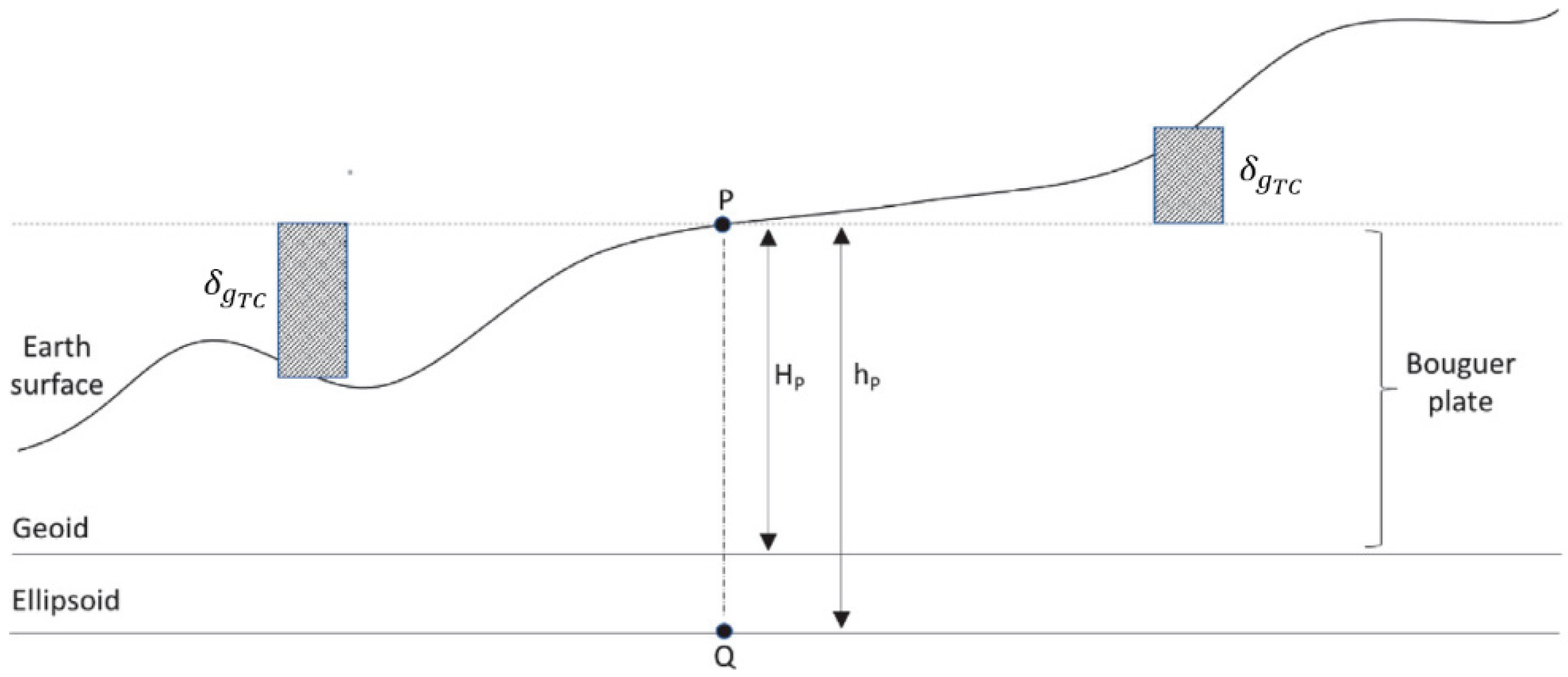
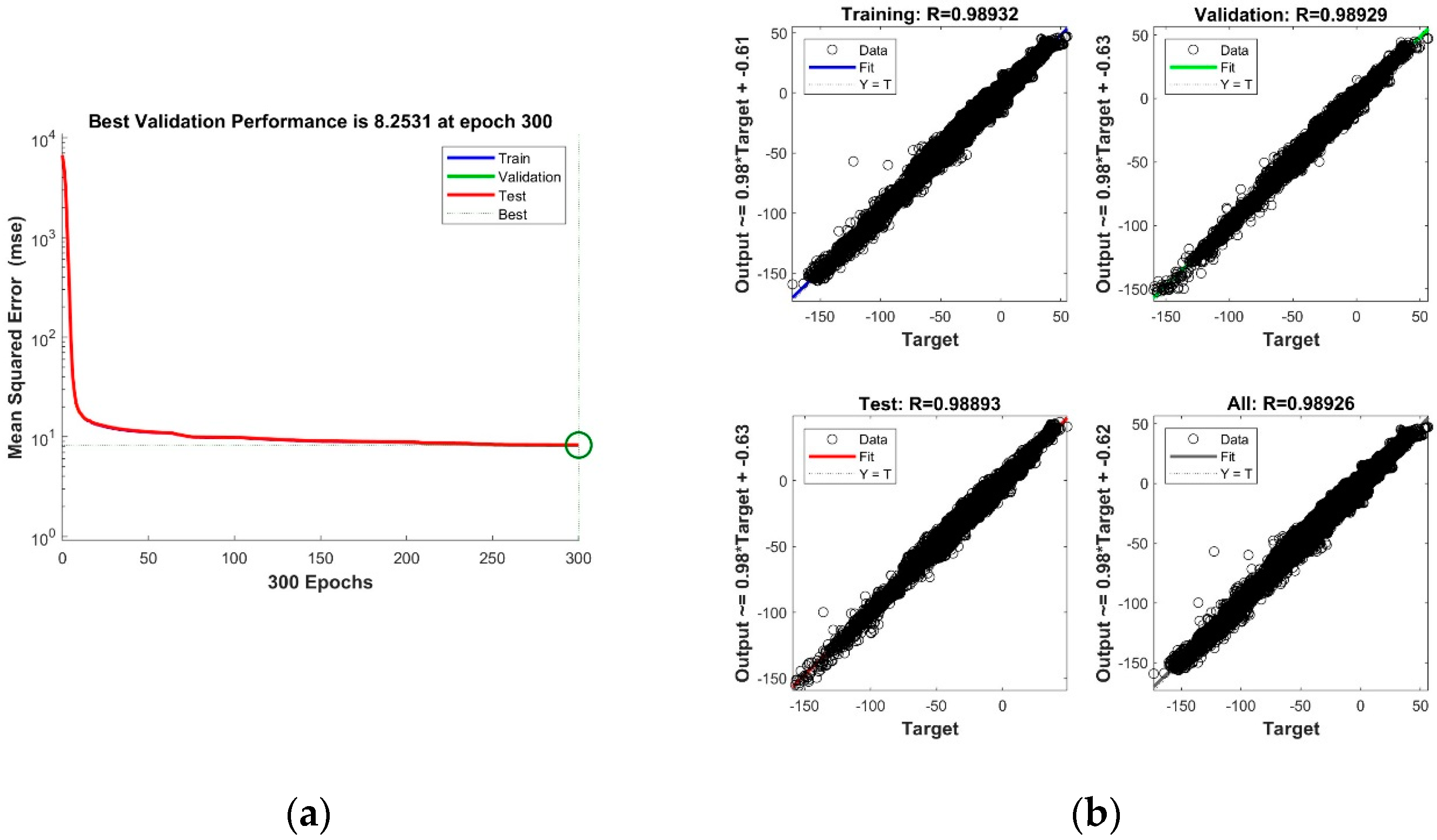
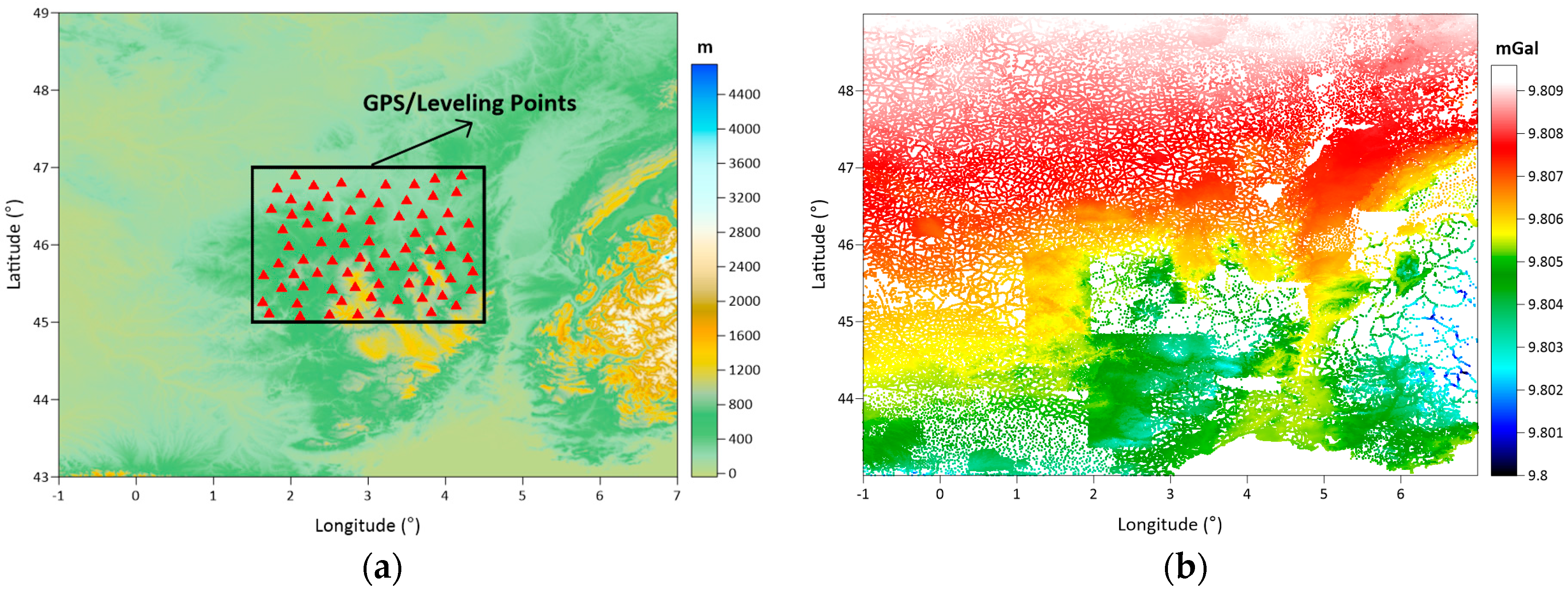
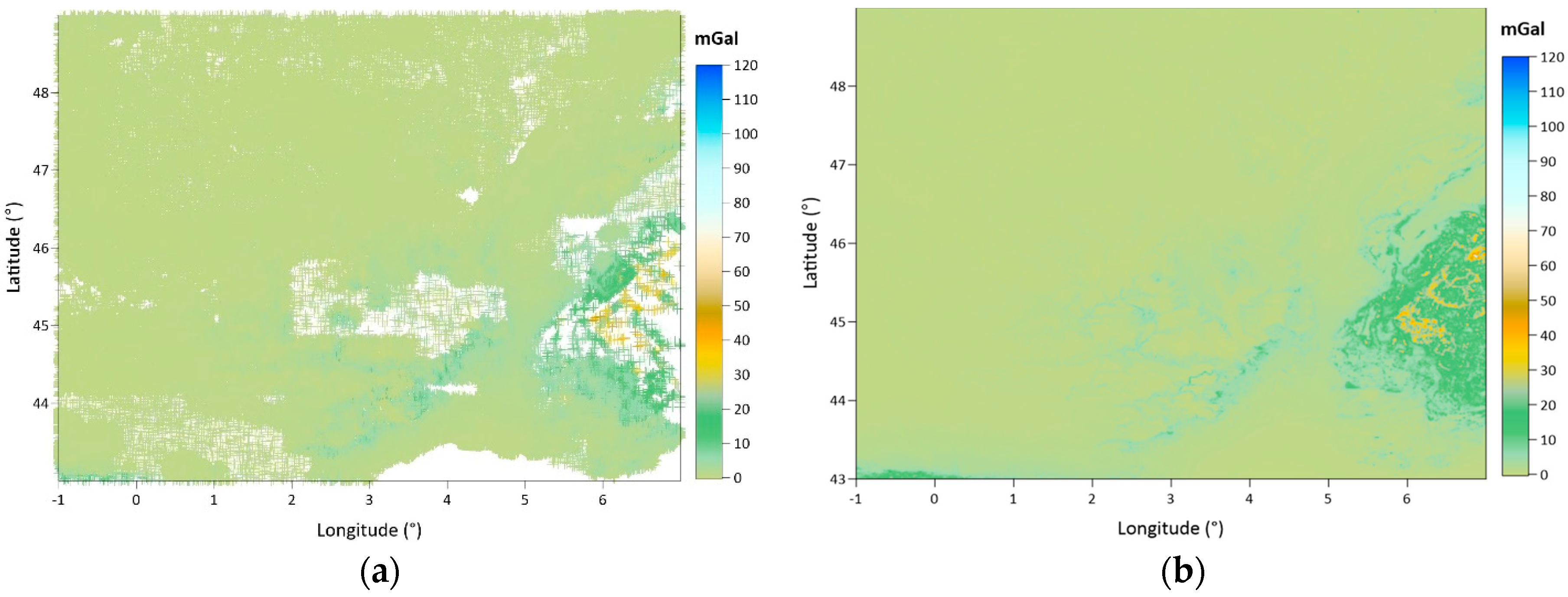
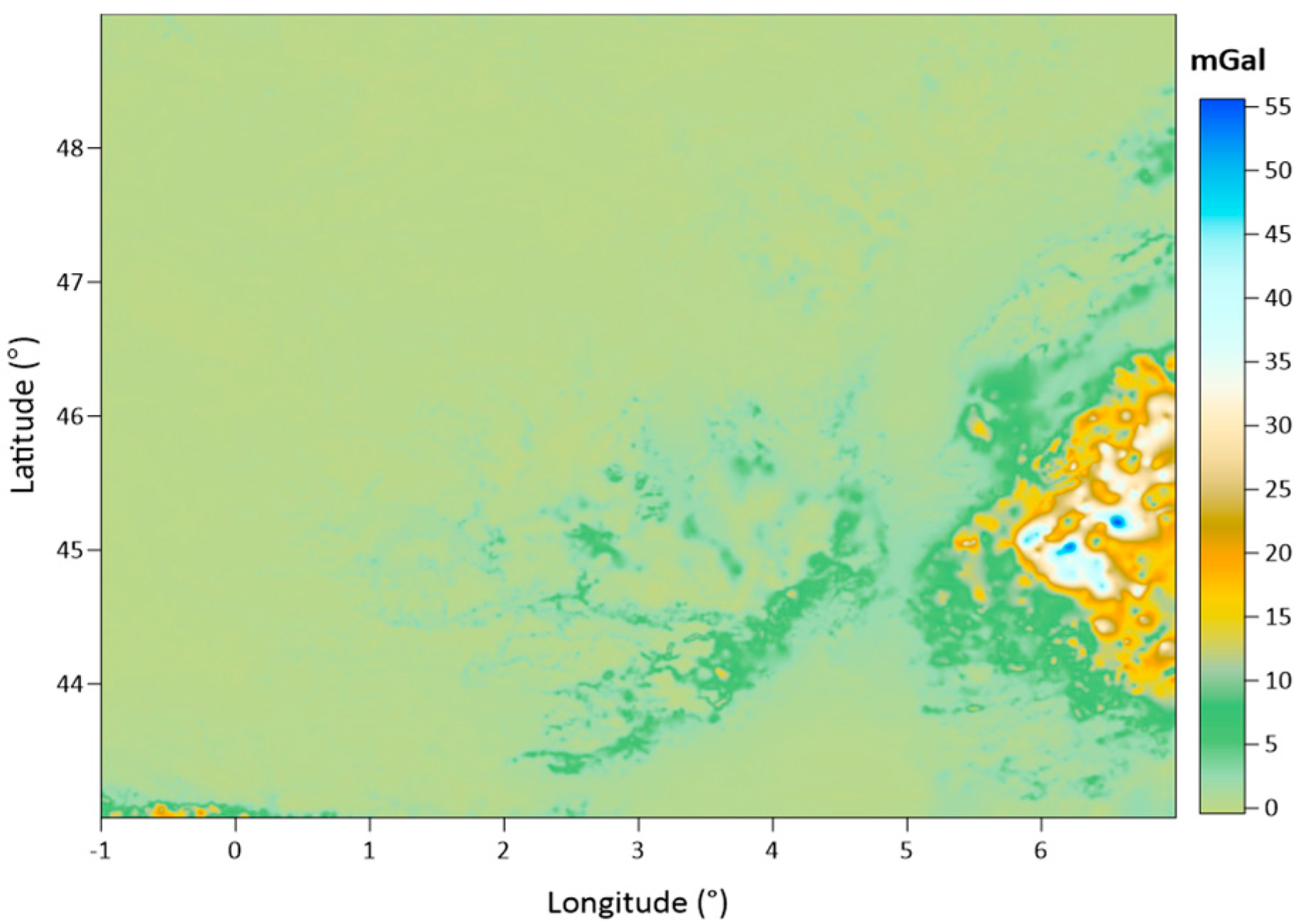
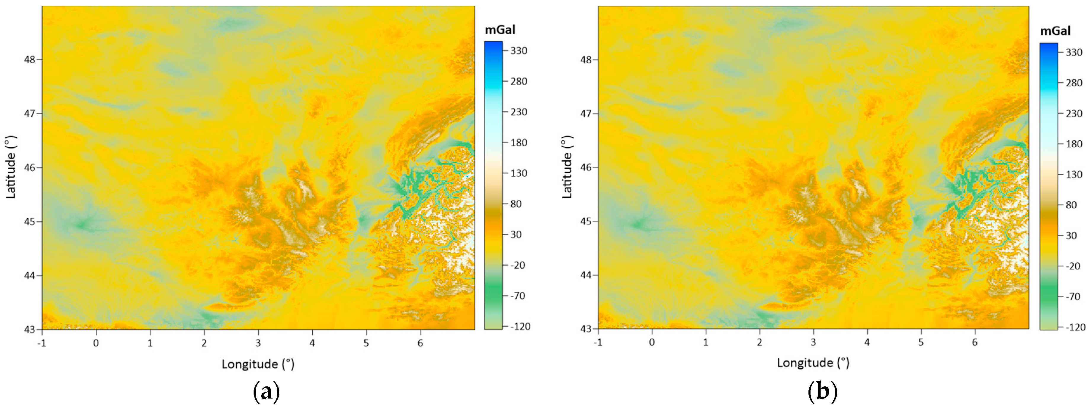
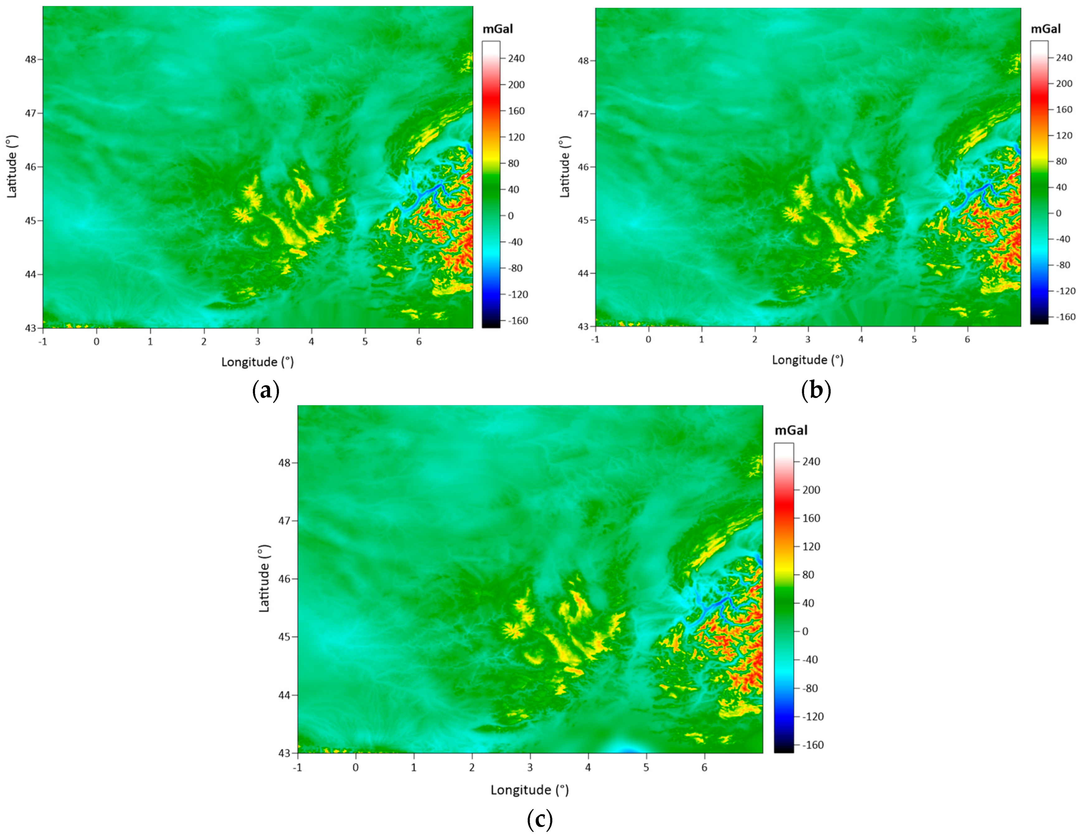
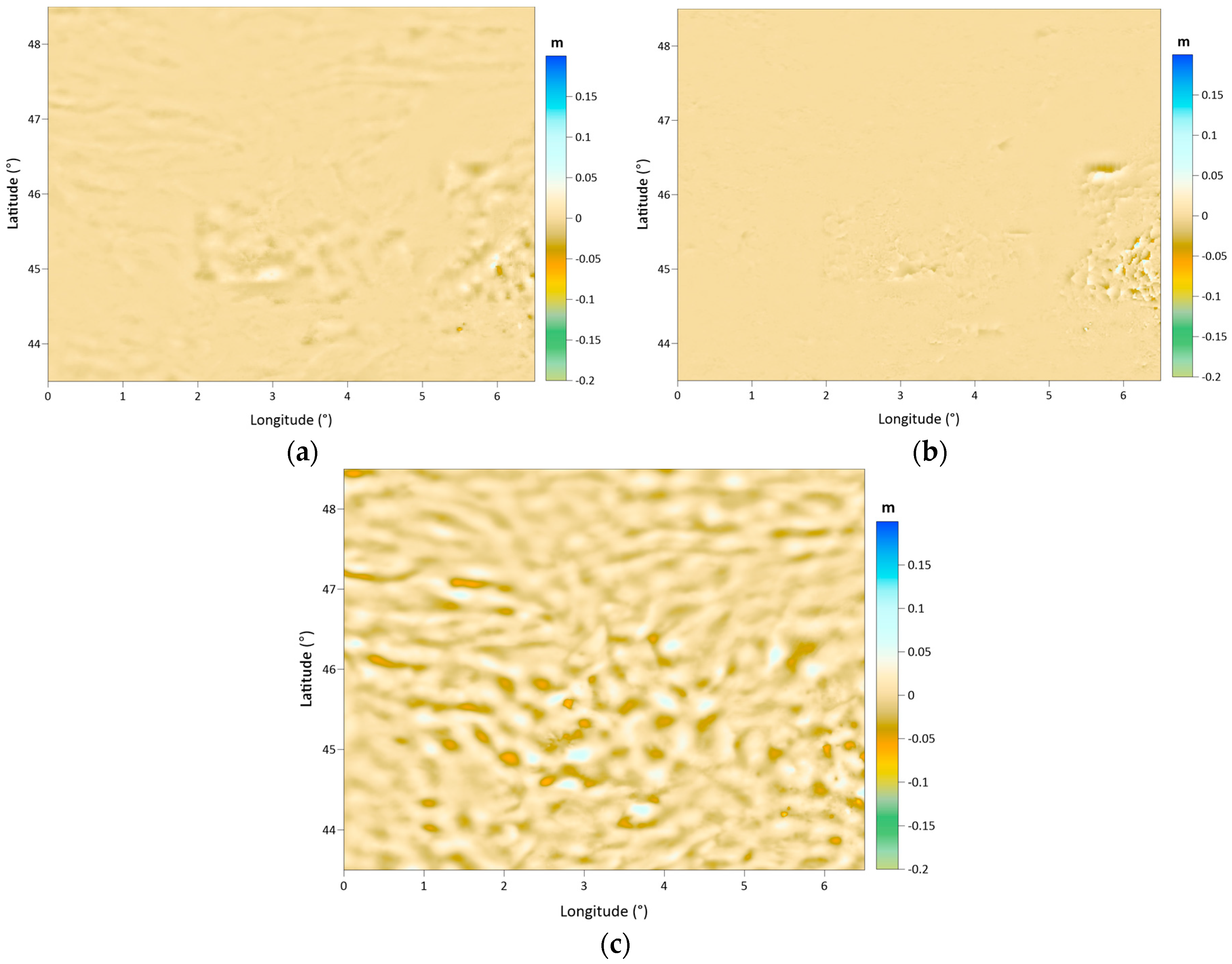
Table 1.
GRS80 (Geodetic Reference System 1980) reference ellipsoid parameters.
| Constant Parameters | Definitions | GRS80 |
|---|---|---|
| Semi-major axis | 6,378,137.0000 m | |
| Semi-minor axis | 6,356,752.3141 m | |
| Normal gravity at equator | 9.7803267715 ms−2 | |
| Normal gravity at pole | 9.8321863685 ms−2 | |
| Geocentric gravitational constant | 3,986,005 × 108 m3 s−2 | |
| First eccentricity | 0.00669438002290 | |
| () | 0.001931851353 | |
| Flattening () | 0.00335281068118 |
Table 2.
Statistics of terrain corrections at the gravity points (point TC) and at the grid nodes (grid TC), and the topographic heights in the area based on the SRTM 3″ DEM data.
Table 2.
Statistics of terrain corrections at the gravity points (point TC) and at the grid nodes (grid TC), and the topographic heights in the area based on the SRTM 3″ DEM data.
| Max | Min | Mean | Median | Std | RMSE | |
|---|---|---|---|---|---|---|
| Point TC (mGal) | 56.533 | −0.317 | 1.043 | 0.476 | 2.153 | 2.392 |
| Grid TC (mGal) | 118.221 | −0.327 | 1.718 | 0.371 | 4.086 | 4.432 |
| 3″ DEM (m) | 4745.649 | −33.506 | 378.900 | 230.454 | 433.149 | 575.485 |
Table 3.
Statistics of the SBAs and CBAs calculated at gravity points and interpolated at 1 arc-minute spacing grid nodes using the Kriging method, and their differences.
Table 3.
Statistics of the SBAs and CBAs calculated at gravity points and interpolated at 1 arc-minute spacing grid nodes using the Kriging method, and their differences.
| Unit: mGal | Max | Min | Mean | Median | Std | RMSE |
|---|---|---|---|---|---|---|
| SBA | 56.373 | −204.830 | −34.170 | −28.652 | 31.640 | 46.569 |
| CBA | 57.271 | −172.656 | −32.238 | −28.097 | 27.905 | 42.638 |
| Difference | 55.590 | −0.439 | 1.932 | 0.396 | 4.879 | 5.247 |
Table 4.
FAA gridding statistics of simple and complete Bouguer anomalies.
| Unit: mGal | Max | Min | Mean | Median | Std | RMSE |
|---|---|---|---|---|---|---|
| FAA (via SBAs) | 345.683 | −126.313 | 8.245 | 1.888 | 29.463 | 30.595 |
| FAA (via CBAs) | 258.962 | −129.942 | 8.458 | 1.948 | 29.867 | 31.042 |
| Difference | 37.167 | −86.721 | 0.213 | 0.016 | 2.103 | 2.114 |
Table 5.
Statistics of geoid models calculated using free air anomalies derived from the SBAs and CBAs grid data.
Table 5.
Statistics of geoid models calculated using free air anomalies derived from the SBAs and CBAs grid data.
| Unit: m | Max | Min | Mean | Median | Std | RMSE |
|---|---|---|---|---|---|---|
| SBA based GEOID | 55.743 | 45.268 | 49.616 | 49.567 | 2.021 | 49.657 |
| CBA based GEOID | 55.470 | 45.267 | 49.616 | 49.567 | 2.021 | 49.657 |
| Difference | 0.273 | −0.195 | 0.000 | 0.000 | 0.008 | 0.008 |
Table 6.
Validation statistics of performed geoid via SBA and CBA grids.
| Unit: m | Max | Min | Mean | Median | Std | RMSE |
|---|---|---|---|---|---|---|
| ∆N SBA | 1.161 | 0.973 | 1.059 | 1.064 | 0.041 | 1.060 |
| ∆N CBA | 1.162 | 0.972 | 1.059 | 1.064 | 0.041 | 1.060 |
Table 7.
Standard deviations of the geoid heights differences from the validations of geoid models calculated using varying and computation parameters.
Table 7.
Standard deviations of the geoid heights differences from the validations of geoid models calculated using varying and computation parameters.
| Unit: m | M = 180 | M = 240 | M = 300 | M = 360 | M = 420 | M = 480 | M = 540 | M = 600 | M = 660 | M = 720 | M = 780 |
|---|---|---|---|---|---|---|---|---|---|---|---|
| Ψ = 0.10° | 0.261 | 0.109 | 0.096 | 0.083 | 0.078 | 0.076 | 0.076 | 0.076 | 0.076 | 0.076 | 0.075 |
| Ψ = 0.25° | 0.174 | 0.146 | 0.142 | 0.139 | 0.131 | 0.112 | 0.102 | 0.085 | 0.072 | 0.067 | 0.065 |
| Ψ = 0.50° | 0.183 | 0.188 | 0.134 | 0.100 | 0.092 | 0.091 | 0.091 | 0.091 | 0.087 | 0.082 | 0.079 |
| Ψ = 0.75° | 0.197 | 0.142 | 0.117 | 0.107 | 0.121 | 0.115 | 0.110 | 0.106 | 0.109 | 0.111 | 0.112 |
| Ψ = 1.00° | 0.197 | 0.158 | 0.153 | 0.172 | 0.175 | 0.166 | 0.167 | 0.183 | 0.188 | 0.195 | 0.192 |
Table 8.
Standard deviations of the geoid heights differences based on the validations of the geoid models calculated with varying error variance parameters.
Table 8.
Standard deviations of the geoid heights differences based on the validations of the geoid models calculated with varying error variance parameters.
| Unit: m | Max | Min | Mean | Std | RMSE |
|---|---|---|---|---|---|
| C = 1 mGal2 | 1.113 | 0.803 | 0.987 | 0.065 | 0.989 |
| C = 4 mGal2 | 1.113 | 0.802 | 0.987 | 0.065 | 0.989 |
| C = 9 mGal2 | 1.113 | 0.801 | 0.986 | 0.066 | 0.989 |
| C = 16 mGal2 | 1.113 | 0.801 | 0.986 | 0.066 | 0.988 |
Table 9.
Standard deviations of the geoid heights differences from the validations of geoid models calculated for different modification choices ().
Table 9.
Standard deviations of the geoid heights differences from the validations of geoid models calculated for different modification choices ().
| Unit: m | Max | Min | Mean | Std | RMSE |
|---|---|---|---|---|---|
| biased | 1.162 | 0.972 | 1.059 | 0.041 | 1.060 |
| unbiased | 1.113 | 0.815 | 0.991 | 0.063 | 0.993 |
| optimum | 1.113 | 0.802 | 0.987 | 0.065 | 0.989 |
Table 10.
Grid statistics belonging to the complete Bouguer anomalies (CBAs) based on the used interpolation algorithms.
Table 10.
Grid statistics belonging to the complete Bouguer anomalies (CBAs) based on the used interpolation algorithms.
| Unit: mGal | Max | Min | Mean | Median | Std | RMSE |
|---|---|---|---|---|---|---|
| Kriging | 57.282 | −172.616 | −32.234 | −28.095 | 27.901 | 42.632 |
| IDP | 55.503 | −172.575 | −32.310 | −28.028 | 27.676 | 42.543 |
| Nearest Neighbor | 56.650 | −173.173 | −32.290 | −28.087 | 27.866 | 42.652 |
| ANN | 55.196 | −159.404 | −32.538 | −27.853 | 27.779 | 42.783 |
Table 11.
Statistics of CBA grid differences between the Kriging grid compared to the IDP grid, nearest neighbor grid, and the ANN grid.
Table 11.
Statistics of CBA grid differences between the Kriging grid compared to the IDP grid, nearest neighbor grid, and the ANN grid.
| Unit: mGal | Max | Min | Mean | Median | Std | RMSE | |
|---|---|---|---|---|---|---|---|
| KRIGING vs. | IDP | 13.646 | −26.880 | 0.076 | 0.009 | 1.314 | 1.316 |
| Nearest Neighbor | 45.066 | −34.711 | 0.056 | 0.006 | 1.618 | 1.619 | |
| ANN | 100.999 | −37.245 | 0.304 | 0.082 | 5.310 | 5.318 |
Table 12.
Statistics of free air anomaly grids obtained from Kriging, the IDP, nearest neighbor and the ANN CBAs grids, respectively.
Table 12.
Statistics of free air anomaly grids obtained from Kriging, the IDP, nearest neighbor and the ANN CBAs grids, respectively.
| Unit: mGal | Max | Min | Mean | Std | RMSE |
|---|---|---|---|---|---|
| Kriging | 258.962 | −129.942 | 8.458 | 29.867 | 31.042 |
| IDP | 266.128 | −128.788 | 8.382 | 29.822 | 30.978 |
| Nearest Neighbor | 266.037 | −132.073 | 8.402 | 29.884 | 31.042 |
| ANN | 256.155 | −128.766 | 8.154 | 30.018 | 31.106 |
Table 13.
Statistics of free air anomaly differences between the Kriging-based grid and the IDP-based grid, nearest neighbor-based grid, and the ANN based-grid, respectively.
Table 13.
Statistics of free air anomaly differences between the Kriging-based grid and the IDP-based grid, nearest neighbor-based grid, and the ANN based-grid, respectively.
| Unit: mGal | Max | Min | Mean | Median | Std | RMSE | |
|---|---|---|---|---|---|---|---|
| KRIGING vs. | IDP | 13.646 | −26.880 | 0.076 | 0.009 | 1.314 | 1.316 |
| Nearest neighbor | 45.066 | −34.711 | 0.056 | 0.006 | 1.618 | 1.619 | |
| ANN | 100.999 | −37.245 | 0.304 | 0.082 | 5.310 | 5.318 |
Table 14.
Statistics of geoid models calculated using free air anomaly grids from the Kriging, the IDP, nearest neighbor, and ANN interpolation methods.
Table 14.
Statistics of geoid models calculated using free air anomaly grids from the Kriging, the IDP, nearest neighbor, and ANN interpolation methods.
| Unit: m | Max | Min | Mean | Std | RMSE |
|---|---|---|---|---|---|
| Kriging | 55.470 | 45.267 | 49.616 | 2.021 | 49.657 |
| IDP | 55.450 | 45.266 | 49.616 | 2.021 | 49.657 |
| Nearest neighbor | 55.462 | 45.267 | 49.616 | 2.021 | 49.657 |
| ANN | 55.451 | 45.264 | 49.616 | 2.021 | 49.657 |
Table 15.
Geoid height difference statistics between the Kriging-based geoid model and the IDP-based, nearest neighbor-based, and ANN-based geoid models.
Table 15.
Geoid height difference statistics between the Kriging-based geoid model and the IDP-based, nearest neighbor-based, and ANN-based geoid models.
| Unit: cm | Max | Min | Mean | Std | RMSE | |
|---|---|---|---|---|---|---|
| KRIGING vs. | IDP | 5.810 | −8.420 | −0.006 | 0.384 | 0.384 |
| Nearest neighbor | 14.240 | −10.050 | −0.001 | 0.408 | 0.408 | |
| ANN | 7.830 | −11.940 | −0.001 | 1.580 | 1.580 |
Table 16.
Validation statistics of the performed geoids.
| Unit: m | Max | Min | Mean | Std | RMSE |
|---|---|---|---|---|---|
| Kriging | 1.162 | 0.972 | 1.059 | 0.041 | 1.060 |
| IDP | 1.164 | 0.974 | 1.059 | 0.041 | 1.060 |
| Nearest neighbor | 1.163 | 0.972 | 1.059 | 0.041 | 1.059 |
| ANN | 1.165 | 0.967 | 1.060 | 0.045 | 1.061 |
Disclaimer/Publisher’s Note: The statements, opinions and data contained in all publications are solely those of the individual author(s) and contributor(s) and not of MDPI and/or the editor(s). MDPI and/or the editor(s) disclaim responsibility for any injury to people or property resulting from any ideas, methods, instructions or products referred to in the content. |
© 2024 by the authors. Licensee MDPI, Basel, Switzerland. This article is an open access article distributed under the terms and conditions of the Creative Commons Attribution (CC BY) license (https://creativecommons.org/licenses/by/4.0/).
Share and Cite
MDPI and ACS Style
Karaca, O.; Erol, B.; Erol, S. Assessments of Gravity Data Gridding Using Various Interpolation Approaches for High-Resolution Geoid Computations. Geosciences 2024, 14, 85. https://doi.org/10.3390/geosciences14030085
AMA Style
Karaca O, Erol B, Erol S. Assessments of Gravity Data Gridding Using Various Interpolation Approaches for High-Resolution Geoid Computations. Geosciences. 2024; 14(3):85. https://doi.org/10.3390/geosciences14030085
Chicago/Turabian StyleKaraca, Onur, Bihter Erol, and Serdar Erol. 2024. "Assessments of Gravity Data Gridding Using Various Interpolation Approaches for High-Resolution Geoid Computations" Geosciences 14, no. 3: 85. https://doi.org/10.3390/geosciences14030085
Note that from the first issue of 2016, this journal uses article numbers instead of page numbers. See further details here.