Lineament Domain Analysis to Unravel Tectonic Settings on Planetary Surfaces: Insights from the Claritas Fossae (Mars)

Abstract

Linear geo-textures are widely recognized on synthetic scaled images of planetary surfaces and consist of elongated alignments of tonal contrasts. When these linear patterns are clustered in azimuthal sets and organized in domains occurring on specific terranes, they reflect the structural grain of the crust and provide clues on the stress trajectories. In this way, the geostatistical analysis of lineament domains represents a useful tool to highlight the geotectonic settings of planetary surfaces. In this work, we applied a lineament domain analysis to better frame the tectonic evolution of the Claritas Fossae (CF) area on Mars, the origin of which is still debated, and both dip–slip and strike–slip tectonics have been described in the literature. A twofold approach was followed that included the identification of a linear pattern with manual and automatic approaches. The automatic method confirmed and validated the results of the manual detection. The statistical analysis of the identified lineaments showed their clustering in two domains that persisted on different terranes separated by the regionally sized scarp associated with the CF. This scarp is the surface manifestation of the CF crustal fault. The spatial distribution of the two domains and their constant angular relationship of about 30° allowed relating one domain to the main CF fault and the other domain to the extensional deformation associated with the fault kinematics. Our results suggest that the CF frames well within a regional setting characterized by right–lateral kinematics with about 20% transtension. Temporal constraints derive from the ages of the terrains where the two domains develop. On this basis, we propose that a first tectonic event occurred in the Noachian age followed by a reactivation occurring after the emplacement of the Late Hesperian lavas.

1. Introduction

The surface morphologies of planetary bodies characterized by a rigid outer shell (e.g., terrestrial planets, icy and rocky natural satellites, etc.) are derived from the contribution and mutual competition of endogenous and exogenous processes. Endogenous processes (e.g., tectonism, volcanism, isostatic adjustments, elastic flexures, among others) shape planetary surfaces yielding the development of sharp topographic contrasts and peculiar tectonic landforms [1,2]. On the other hand, impact cratering and erosion, transport, and depositional processes related to climatic conditions (active on planets with atmosphere) tend to smooth and obliterate landforms created by endogenous processes. In this way, studying the variety of planetary landforms provides fundamental information on the geological history of a planet. Despite the increasing number of planetary missions (that include the use of landers and rovers for direct in situ/local measurements, drilling, and sampling), tectonic and geodynamic investigations on planetary bodies mainly rely on indirect, orbital data. Such studies usually use methodologies developed and successfully applied to unravel the geotectonic setting of key regions on Earth where access for direct investigation is difficult for climatic, economic, or geopolitical reasons. These methodologies include the study of potential fields [3,4,5,6], heat flux [7,8,9], and surface geo-textures from remotely sensed data [10,11,12,13,14].

Regionally sized lineaments (with lengths of the order of hundreds to thousands of kilometers) detected on synthetic scaled images of deformed regions record the signature of tectonic deformations, thus providing a useful tool to highlight their geotectonic evolution. Azimuthal and spatial analyses of lineaments provides fundamental insights to applied studies, such as the characterization of hydrothermal fluid circulation [15,16] and groundwater fractured reservoirs [17,18,19], assessment of hydrocarbon potential in oil fields [20,21], characterization of areas with high landslide susceptibility [22,23], and investigation of the structural settings of seismically and volcanically active regions [24,25,26], as well as to unravel the tectonic evolution of different planetary surfaces [13,27,28,29,30,31,32,33,34]. During the last decades, quoting [35], “definitions and theories on the origin of lineaments have been almost as numerous as the lines themselves” (see also [36] for a review on the various definitions of lineaments since [37]). In the present paper, we refer to lineament textures that are elongated alignments of image tonal contrasts consisting of the population of subparallel lineaments. These satellite-scale lineaments are tens to hundreds of kilometers long, cluster in azimuthal family sets called domains, and persist over wide regions (hundreds to thousands of square kilometers) forming lineament swarms. This description resembles the definition of lineaments given by [35], and they are described as originating from the weathering and erosional etching of subtle features produced by the extension of the brittle upper crust above a deeper layer behaving in a more ductile fashion. The importance of this class of lineaments is emphasized by their membership in a large population. Therefore, this kind of lineament texture analysis does not focus on the geo-tectonic meaning of a single lineament; instead, it is based on the characteristics of the entire population. In fact, the inclusion, omission, or misinterpretation of one or a few single lineaments does not affect the tectonic meaning of the entire population [35]. Multiple sets of lineament textures (e.g., domain) may exist in the same region, thus producing the structural/topographic grain of the region. In this way, these lineament textures reflect the structural architecture of the crust that in some cases is partly hidden by thick sedimentary or ice covers. Nevertheless, the dynamic adjustment of such covers (including sediment compaction and ice flow) records on their surface the architecture of the bedrock, and this smoothed signature may be detected and analyzed well from satellite-scale images [11]. Following [35], lineament domains represent the surface manifestation of crustal stress trajectories. Specifically, under Andersonian stress conditions, the main lineament domain develops perpendicularly to the least horizontal compression (σ2 in compressional regimes, and σ3 in extensional and strike–slip regimes) and parallel to the maximum horizontal compression (σ1 in compressional and strike–slip regimes, and σ2 in extensional regimes). In this way, the characteristics and spatial distribution of lineament domains and swarms have been observed reflecting crustal geodynamic effects on different planetary surfaces (e.g., Earth: [16,38,39,40,41]; Ganymede: [13,14]; Mars: [28,42,43,44].

In the present study, we conducted a lineament domain analysis (sensu [35]) in the Claritas Fossae (CF) region of Mars. This is a highly deformed area in which the role of tectonics is still debated. We followed a manual and an automatic approach with the aim of better framing the tectonic evolution of the region. Both analyses converged into similar results confirming the reliability of the method in unravelling the tectonic evolution of planetary surfaces.

2. Geological Setting

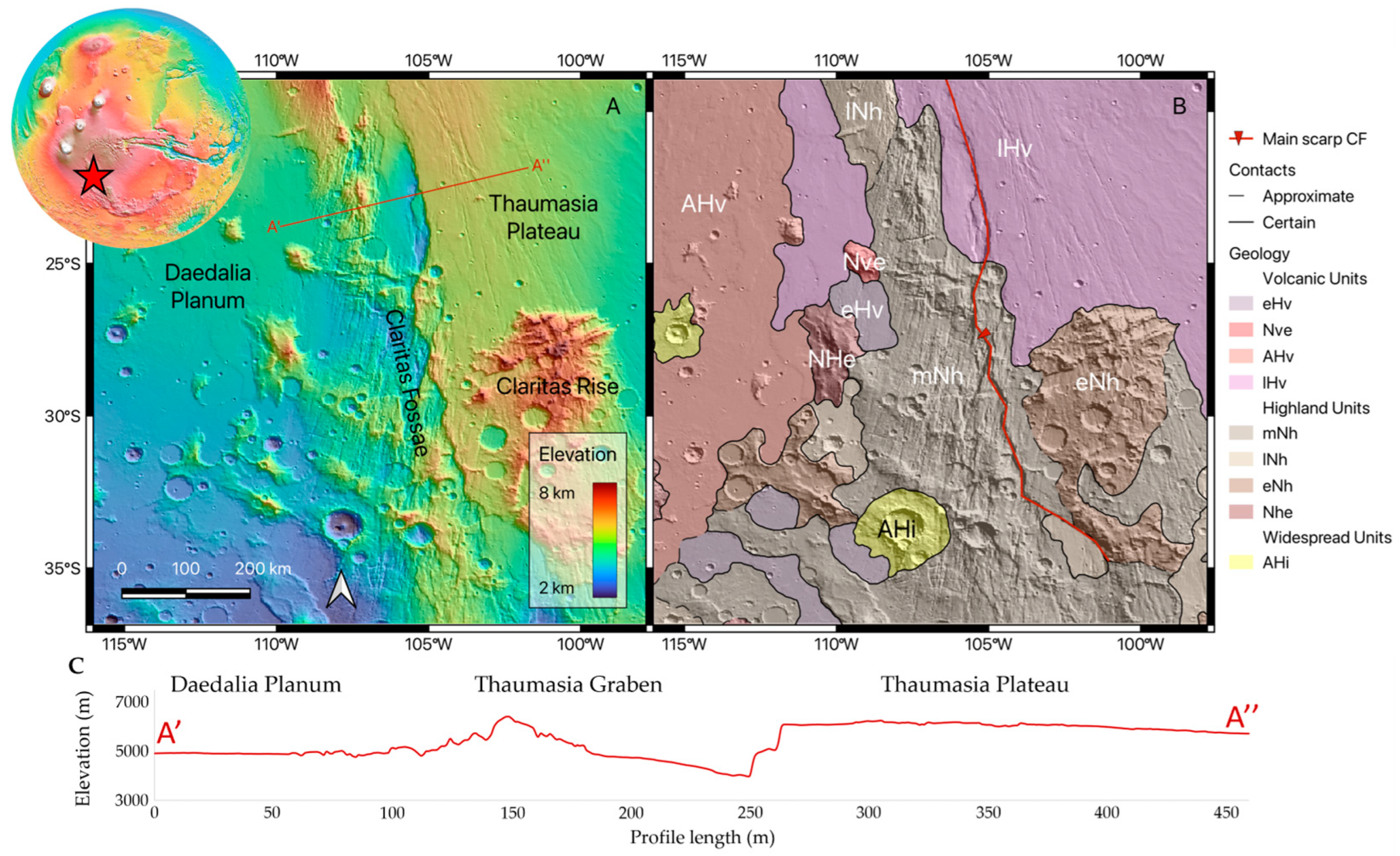
The Claritas Fossae, hereinafter referred to as the CF, represents the westernmost boundary of the Thaumasia region between 15° S–40° S and 95° W–115° W (Figure 1A). It consists of an intricate, NNW-SSE-elongated system of scarps, ridges, and depressions that exceeds 1000 km in length and 150 km in width. The CF develops between the heavily deformed Noachian terrains and the Late Hesperian terrains of the Thaumasia Plateau (Figure 1B) [45,46,47,48]. Regionally, the CF features an asymmetric valley (namely, the Thaumasia Graben, or TG, defined by [49]) that is bounded to the east by a west-dipping, steep scarp and to the west by a gently rounded slope (Figure 1C). The scarp is a striking physiographic feature that develops for more than 900 km in length on both the Noachian and Late Hesperian terrains. It marks an abrupt elevation change that exceeds 2000 m between the valley bottom of the TG and the Thaumasia Plateau. In plain view, it is characterized by a series of en-echelon segments that mostly characterize the southern Noachian terrains. The scarp separates two areas with different textures: to the west, a pervasive network of depressions, scarps, fractures, and graben- and half-graben-like morphologies result in a rough landscape; to the east, depressions and graben-like morphologies are more widespread, outlining a smoother landscape. Due to its morphometric characteristics and dimensions, the scarp is considered by different authors as the surface expression of a crustal-scale tectonic structure strictly related to the development of the CF [49,50,51].

The origin of the CF has been related to one or multiple tectonic deformations that acted between the Noachian and Amazonian ages [46,49,50,51,52,53]. Different tectonic settings have been proposed on the basis of the morphological characteristics of the area. The asymmetric architecture of the TG, which resembles half-graben-like morphologies, has led different authors to propose an extensional tectonic setting developed in one long-standing stage or during multiple events [46,52]. In this scenario, the regional dimension and the morphometric characteristics of the scarp suggest the presence of a crustal-scale listric normal fault responsible for the development of the half-graben morphology [49,51,54,55,56]. In addition to this evidence, in the area of the CF, Riedel-type arrangements and en-echelon patterns can also be recognized, suggesting that strike–slip kinematics likely contributed to the present-day setting [50,51,57].

Although the type of the deformation/kinematics is still debated, authors are concordant on the tectonic nature of the CF. In favor of the proposed scenarios, several terrestrial analogues have been highlighted such as the Kenya Rift and the Icelandic Rift for the extensional setting [49,51], and the Western North American margin and the Sant Andreas Fault for the strike–slip kinematics [57,58,59].

3. Materials and Methods

In the present work, lineament domains (sensu [35]) were analyzed following a manual and automatic approach. The proposed methodology was aimed at identifying the lineament domains that exist in the area of the CF in order to provide original constraints to frame the tectonic evolution of the area. In particular, the automatic approach, which was successfully used on other planetary surfaces [13,32], was here applied to confirm the results of the manual detection. In this way, comparable results of the two approaches granted robustness to the dataset and strengthened the tectonic interpretations.

3.1. Manual Lineament Detection and Statistical Analysis

Lineaments outcropping in the study area were visually identified through the photogeological interpretation of satellite image mosaics. Lineaments appeared as patterns of aligned pixels reflecting linear anisotropies in the image texture. To ease their identification, an ad hoc image enhancement [39,60] was conducted with the Digital Elevation Model (DEM) derived from the acquisitions of the Mars Orbiter Laser Altimeter (MOLA) aboard the Mars Global Surveyor (MGS), namely the Mars MGS MOLA DEM 463 m v2 dataset [61,62]. This dataset has 463 m/px of spatial resolution, represents the best compromise between scale and resolution, and provides a synoptic view of the study area while preserving the signature of regionally sized tectonic features. In the geographic information system (GIS) environment, based on the open-source software QGIS_3.30_s-Hertogenbosch, from the original dataset, a subset of the study area was extracted. It represented an area of 1060 × 1080 km in the latitude interval of 20°–35° S and longitude interval of 100°–115° W. The subset image was resampled at a spatial resolution of 1000 m/px. In this way, the image was filtered to exclude elements and morphologies related to local effects that we considered negligible for the regional aim of this work. Shaded relief images were derived from the resampled subset image according to four low-angle (20°) synthetic lighting conditions trending 45°, 90°, 135°, and 180° (Figure 2). This allowed the reduction of the bias induced by a single direction of the light for which lineaments nearly parallel to the direction of the light tend to be hidden and those nearly perpendicular emphasized [16,29,63,64]. Linear texture enhancing of each shadow image included (i) the application of a Laplacian filter to emphasize higher spatial frequency related to the presence of the tectonic texture; and (ii) a lookup table stretching to enhance the tone contrasts and ease the manual identification of the lineaments [65].

Lineaments detection was conducted in a GIS environment (QGIS_3.30_s-Hertogenbosch) through the systematic visual inspection of each enhanced shadow image and following the rules provided in [66]. Thus, four distinct lineament datasets were derived. Due to the regional purpose of the present work, only lineaments corresponding to pixel alignments that maintained the same azimuthal direction for no less than 20 km were traced. Identified lineaments were digitized by manually tracing linear elements by drawing vertices by clicking on a fixed map scale of 1:10,000,000. The linear, digital elements were stored in four dedicated vector layers. The following attributes were calculated for each lineament: length, azimuthal direction, and the coordinates of the extremes and of the centroids. The four derived datasets including the lineaments identified in the four shadow images were then grouped into a single database. This database was statistically analyzed using Daisy3 software (v. 5.58.3.231121, Rome, Italy). Daisy3 allowed us to conduct an azimuthal analysis by frequency and cumulative length following the approach presented in [67]. This analysis included the polymodal Gaussian fit aimed at identifying the main azimuthal family set (i.e., lineament domains, sensu [35]). The statistical analysis includes several steps: (i) the histograms of the azimuth by the frequency and cumulative length of the identified lineaments were prepared and normalized to their highest value; (ii) the histograms were smoothed to reduce the statistical noise by a selected number of moving weighted averages [68,69]; (iii) the peak(s) of the histograms were fitted with the sum of the Gaussian curve functions using a best-fit algorithm [70]; (iv) the results were plotted as rose diagrams that represented as “petals” the recognized unimodal- (single azimuthal cluster) or polymodal-distribution (multiple azimuthal clusters) lineament domains. In this way, each domain could be described by its Gaussian/statistical parameters, such as the main azimuth, standard deviation, and relative height. In particular, the value of the standard deviation (SD), calculated as the width of the petals/Gaussian measured at half height, was related to the azimuthal scattering of the lineament domains. Two domains were easily identified when their angular distance (i.e., the distance between their modes) was higher than their SD and thus the corresponding Gaussian peaks showed minimal or null overlap.

3.2. Automatic Lineament Detection and Statistical Analysis

Criticism about lineament detection relies on the magnitude of its potential for observer bias [66]. In fact, manual lineament identification may be conditioned by psychological factors of operators, such as an enthusiasm for drawing lines or former knowledge of the study area that could produce a biased dataset. For this reason, automatic detection was performed to strengthen the objectivity of the dataset manually traced. In the present work, SID software (v. 3.06-2, Rome, Italy) [71] was used. It is of note that this software has been successfully used in previous geotectonic investigations both on Earth and on other planetary surfaces [11,12,13,32,39,40]. The SID software was used to discover the alignment of the adjacent-pixel contrast in the pre-processed DEM (Mars MGS MOLA DEM 463 m v2) of the Martian surface by a systematic search for all possible digital combinations of segment directions within a given range of parameters. According to the used parameters, the algorithm can identify faint, discontinuous lineaments characterized by alignments of the adjacent-pixel contrast separated by null pixels. The software searched for lineaments according to a set of parameters defining the characteristics of the linear pattern. These parameters included: the minimum and maximum length of a pixel unit of a lineament; the width of the lineament in pixel units measured perpendicularly to its strike; the dimension of the moving smoothing window along the potential lineament to override the discontinuities in pixel distribution; the minimum length of each lineament segment; the maximum distance between lineament segments that belonged to the same lineament; and the pixel density along the lineaments.

In this study, a set of parameters was selected to discover lineaments longer than 30 km and 3 km wide. The ad hoc image enhancement of the four shadowed images (prepared as described in the previous section) included: (i) Laplacian filtering (to emphasize the higher spatial frequency related to the presence of the linear texture); (ii) threshold slicing (to select pixels contributing to the image texture related to the presence of lineaments and in order to reduce the meaningful pixel number to ~10% of the image); (iii) and LIFE filtering (that allowed a reduction in random noise in the raster image). The resulting images were then automatically processed with SID to recognize lineament patterns. The detected lineaments were cumulated into a database that was successively statistically analyzed through the Daisy3 software (v. 5.58.3.231121, Rome, Italy) to discover lineament domains with the same procedure previously described.

4. Results

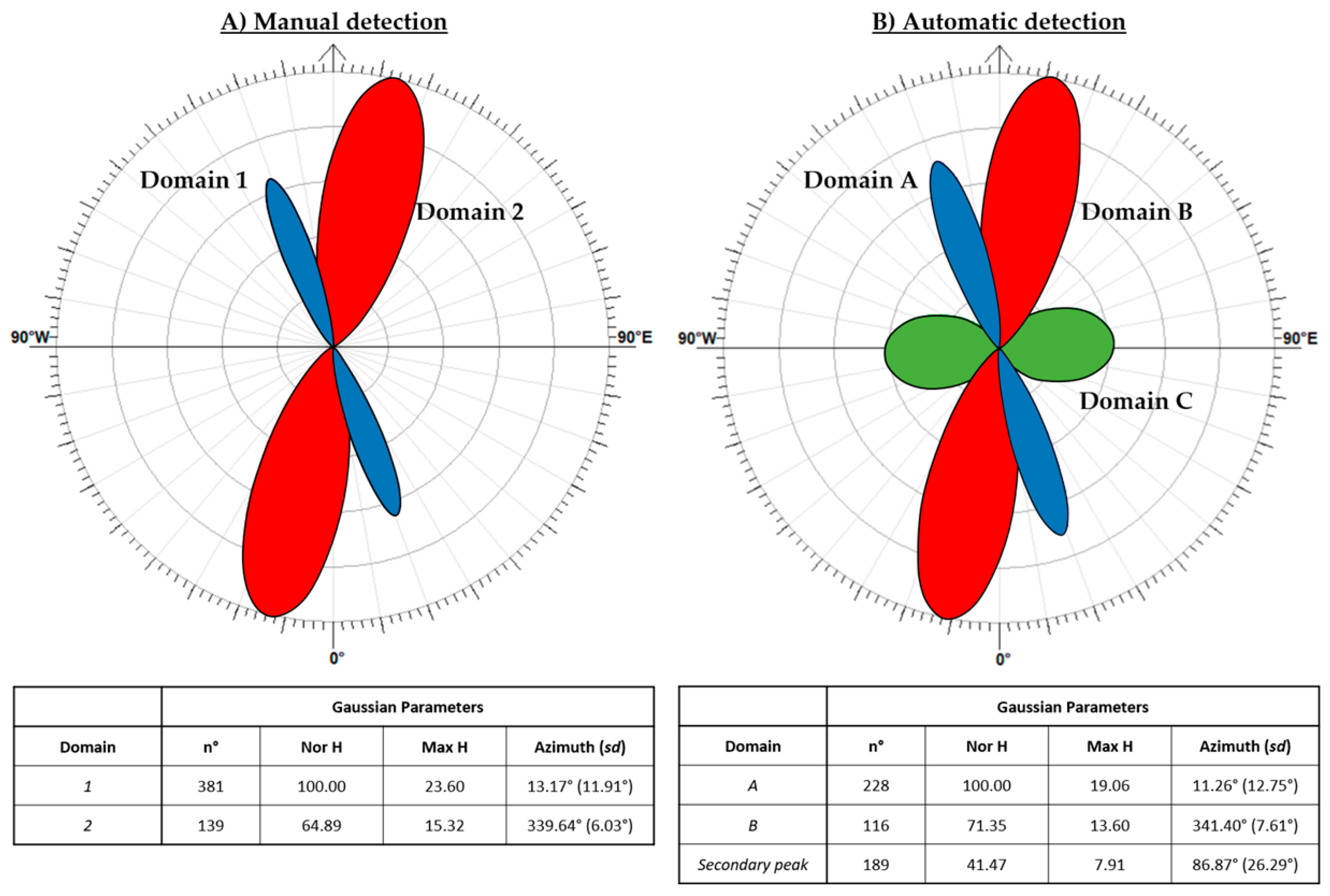
The photogeological interpretation of the four shadow images allowed the visual identification of 735 lineaments (Figure 3A). The polymodal Gaussian fit highlighted that the identified lineaments were not randomly distributed but clustered around two preferential orientations, thus defining two lineament domains (sensu [35]). The two lineament domains were clearly highlighted by both the analyses by frequency (upper part of the rose diagrams in Figure 3B and Figure 4A) and by cumulative length (lower part of the rose diagrams). They are (i) Domain 1 (red), which included 381 lineaments with a main azimuthal direction of 13.39° (NNE-SSW), SD: 11.91°; and (ii) Domain 2 (blue), which included 139 lineaments with a main azimuthal direction of 339.35°(NNW-SSE), SD: 6.03°. The angular difference between the two Gaussian peaks was 34.04°, which was well above the SD of both the domains. This indicated that the analysis identified two separated Gaussian peaks that represented two distinct, non-overlapped lineament domains. In addition, Figure 3B shows that Domain 1 and 2 were characterized by different spatial distributions. Domain 1 was spatially clustered in the western part of the study area, whereas Domain 2 was clustered in the eastern part.

The automatic lineament domain analysis identified 824 lineaments. The polymodal Gaussian fit highlighted two main Gaussian peaks corresponding to two lineament domains and a minor peak (Figure 4B) that were (i) Domain A (red), which included 228 lineaments with a main azimuthal direction of 11.26° (NNE-SSW), SD: 12.75°; (ii) Domain B (blue), which included 116 lineaments with a main azimuthal direction of 341.40°(NNW-SSE), SD: 7.61°; and the third, secondary peak, which included 189 lineaments with a main azimuthal direction of 86.87° (E-W), SD: 26.29°. Domains A and B strictly resembled Domains 1 and 2 identified through the manual approach. The strong azimuthal similarity is shown in Figure 4 and confirmed the reliability of the manually traced lineaments. Therefore, in the following discussion and tectonic interpretations, the manual lineament dataset will be used. The rose diagrams in Figure 4 show that the azimuthal differences between Domains 1 and A, and 2 and B were less than 2°. Thus, also the mean angular distance between Domains A and B, which was 29.86°, was nearly the same as that between Domains 1 and 2 (34.04°) with a difference less than 5°.

5. Discussion

The two detected lineament domains (i.e., NNE/red and NNW/blue) persisted over two distinct areas separated by the main TG scarp (Figure 3). The different spatial distribution is shown with density maps created for each domain in Figure 5. The density maps were obtained in a GIS environment (QGIS_3.30_s-Hertogenbosch) through the plugin “Heatmap” that used the kernel density estimation algorithm to generate a density raster from a vector point layer as an input. The density of the points was calculated as a function of the number of points in a position. The more points that were present, the larger the values. In our study’s case, the centroids of the lineaments were used as points for the input layer. The density map in Figure 5A shows an almost homogenous distribution of the NNE domain to the west of the major scarp of the TG, in correspondence to the Noachian terrains (an area with a slightly higher concentration can be observed around 28° S and 103° W). On the other hand, the density map in Figure 5B highlights that the NNW domain was characterized by two areas with higher concentrations of lineaments to the east of the major scarp of the TG. The main concentration was located to the north of the Claritas Rise, where lHv crops out. The secondary concentration was to the south and persisted from the Early to Middle Noachian terrains. A local minimum of the NNW domain occurred in correspondence to the Claritas Rise.

As shown in Figure 3B and Figure 5, the transition between the two domains was sharp and occurred in correspondence to the major scarp of the TG. This last was a regional tectonic lineament considered the superficial manifestation of a crustal-scale tectonic feature [51]. Specifically, some authors have argued for the existence of a crustal-scale listric normal fault that developed in an extensional tectonic setting; others have proposed that a regional shear corridor developed in a right-lateral strike–slip regime [49,50,51,57]. Following our analysis, the NNW domain included some strands of the major scarp of the TG [51] and shared with the scarp the same orientation (Figure 3B). However, the prevailing lineament domain in the area of the CF was found to be in the NNE domain. According to [35], the main lineament domain under Andersonian stress conditions developed perpendicularly to the least horizontal compression (or parallel to the maximum horizontal compression). In this way, in an extensional tectonic scenario, the extension should be WNW-ESE-oriented, which would not be compatible with the NNW-SSE regional orientation of the CF. An important clue for the tectonics of the CF was related to the angular relationship between the two identified domains. In particular, the low values of SD that characterized both the NNE and NNW domains indicated a small azimuthal scattering of the identified lineaments. Thus, the angular relationship, which was ~30°, was maintained for the entire extent of the CF (>1000 km in length and >150 km in width). According to [12,13], in pure strike–slip tectonic regimes, the angle between the main fault/shear corridor and the maximum horizontal compression induced by kinematic conditions was 45°. The angle reduced or increased in the case of transtensional or transpressional kinematics, respectively (Figure 6). In this way, the variation of the fault kinematics yielded the rotation of the angle of the intra-fault/shear corridor stress field resulting in a different orientation of the related lineament domain (Figure 6A). In the case of our study, the angle of ~30° between the NNE and NNW domains suggested that the identified domains developed in a transtensional tectonic regime. This tectonic reconstruction was also supported by the sketch presented in Figure 6B, in which the acute angle θ between the shear corridor and the related fractures/lineaments was used to quantify the transtensional/transpressional components of a strike–slip corridor. In the case of our study, the angle of ~30° referred to a right-lateral transtensional regime characterized by a ~20% extensional component.

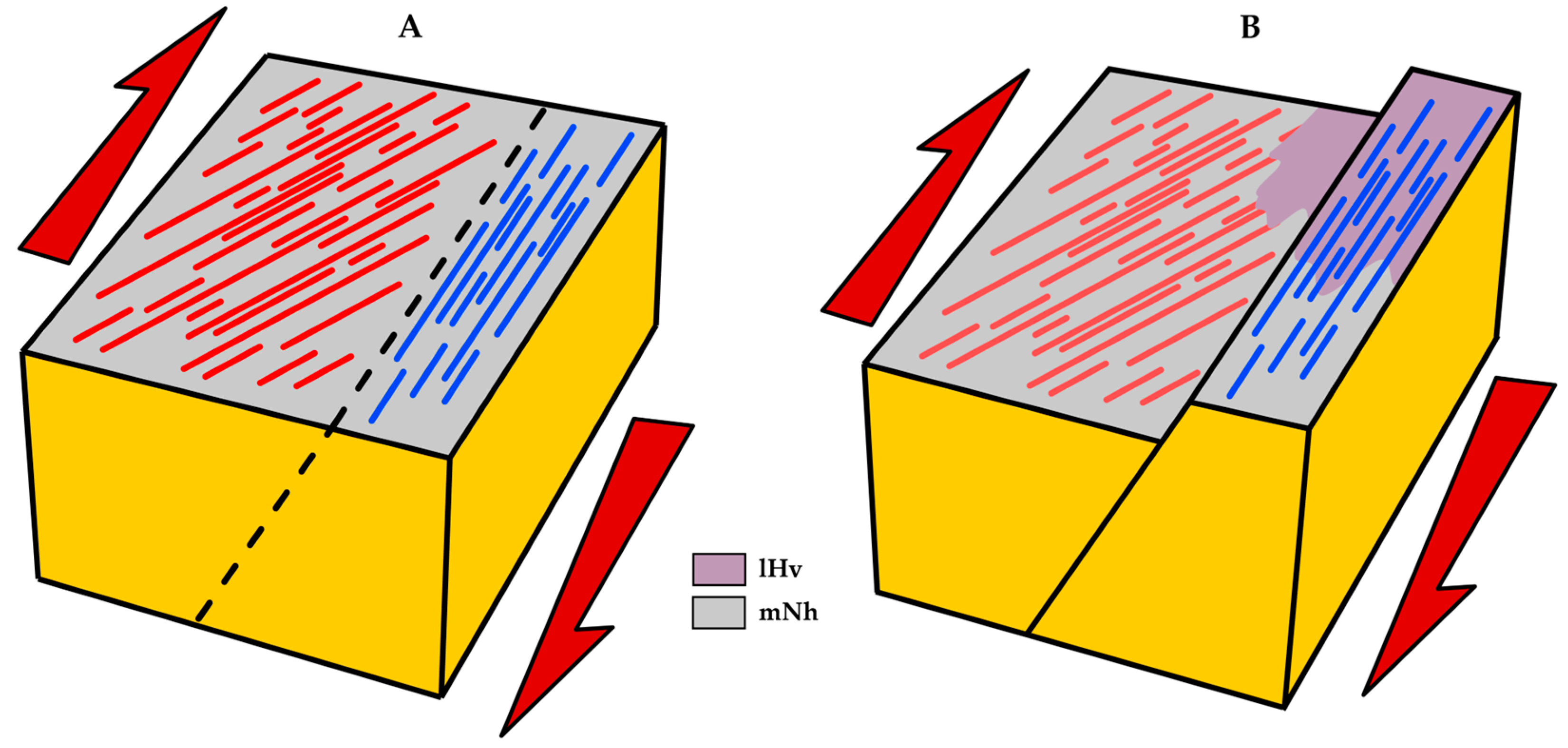
Additional information can be derived from the polymodal Gaussian fit analysis that could be used to determine the relative age of the identified domains [11,72]. In particular, the ratio between the values of the normalized Gaussian height NorH and standard deviation SD (values for both domains are shown in tables in Figure 4) was indicative of the sharpness of the peaks or, in other words, of the azimuthal scattering of lineaments belonging to the same domain with respect to their frequency [60]. Exogenous processes that act on areas deformed by tectonic/endogenous processes tend to increase the azimuthal scattering of the original unaltered linear geometries, thus increasing the SD of the domain [11,60,72]. Therefore, higher values of NorH/SD relate to relatively younger lineament domains [11,60,72]. In the case of our study, NorH/SD was higher for the NNW domain (NNE 8.39 and NNW 10.76). This indicated that the NNW domain was relatively younger compared to the NNE domain. This was also supported by the spatial distribution of the domains as highlighted by the density maps that show the NNW domain developing on both the Noachian and Late Hesperian terrains, whereas the NNE domain persisted only over the Noachian terrains. This evidence suggested the formation of NNE domain in the Noachian age and the NNW domain after the onset of the Late Hesperian age. This disagreed with the coeval or nearly coeval growth of both domains in a single tectonic stage, whereas it could be better explained by a tectonic evolution comprising multiple events in accordance with [51]. In this multi-phase tectonic scenario, a first right-lateral transtensional event led to the development of both the domains during the Noachian age. A subsequent event occurred after the emplacement of the Late Hesperian lavas and likely reactivated the NNW domain, thus explaining its younger relative age. This tectonic reconstruction is in line with the beginning of the tectonic deformation at the CF in the Noachian age proposed by different authors (e.g., [46,52]), and with the event that yielded the development of the TG between the Late Hesperian and Early Amazonian ages [49,73]. In Figure 7, the proposed tectonic evolution that led to the formation of the two identified domains is shown. In this way, the lineament domain analysis proved to be a powerful tool to highlight the crustal stress of the deformed regions. Specifically, the stress directions highlighted by the NNE domain were compatible with a kinematically induced stress in an NNW-SSE regional corridor of deformation characterized by dextral shear. These findings were in accordance with the evolutionary model proposed in [51] and with the preliminary results on the spatial distribution of the three major fault trends identified in [74]. In particular, this different, independent dataset provides similar results that strongly support a polyphase tectonic evolution of the CF. Similar tectonic reactivations along inherited weakness zones are a deeply investigated deformation process that operates both on Earth (e.g., [75,76,77]) and on other planetary surfaces (e.g., [13,27,32]).

6. Conclusions

In this work, we applied a manual and an automatic approach to conduct a lineament domain analysis to investigate the CF, a complex, tectonically controlled area representing the western boundary of the Thaumasia Region. Through a polymodal Gaussian fit analysis, the existence of two lineament domains was highlighted: the NNE domain and NNW domain. The angular relationship between the domains indicated that the domains developed within a right-lateral transtensional tectonic regime during the Noachian age. The relative age of the domains, as derived from the NorH/SD ratio, suggested a possible reactivation of the NNW domain between the Late Hesperian and Early Amazonian ages. This is in line with a polyphase tectonic evolution of the CF. Eventually, the lineament domain analysis proved to be a free and a real-time method to investigate tectonically controlled areas, both in manual and automatic approaches.

References

- Gutiérrez, F.; Gutiérrez, M. Landforms of the Earth: An Illustrated Guide; Springer: Cham, Switzerland, 2016. [Google Scholar]
- Rossi, A.P.; van Gasselt, S. Geology of Mars after the first 40 years of exploration. Res. Astron. Astrophys. 2010, 10, 621. [Google Scholar] [CrossRef]
- McKenzie, D.; Barnett, D.N.; Yuan, D.N. The relationship between Martian gravity and topography. Earth Planet. Sci. Lett. 2002, 195, 1–16. [Google Scholar] [CrossRef]
- Langlais, B.; Purucker, M.E.; Mandea, M. Crustal magnetic field of Mars. J. Geophys. Res. Planets 2004, 109, E2. [Google Scholar] [CrossRef]
- Morschhauser, A.; Lesur, V.; Grott, M. A spherical harmonic model of the lithospheric magnetic field of Mars. J. Geophys. Res. Planets 2014, 119, 1162–1188. [Google Scholar] [CrossRef]
- Genova, A.; Goossens, S.; Lemoine, F.G.; Mazarico, E.; Neumann, G.A.; Smith, D.E.; Zuber, M.T. Seasonal and static gravity field of Mars from MGS, Mars Odyssey and MRO radio science. Icarus 2016, 272, 228–245. [Google Scholar] [CrossRef]
- Grott, M.; Hauber, E.; Werner, S.C.; Kronberg, P.; Neukum, G. High heat flux on ancient Mars: Evidence from rift flank uplift at Coracis Fossae. Geophys. Res. Lett. 2005, 32, 21. [Google Scholar] [CrossRef]
- Grott, M.; Hauber, E.; Werner, S.; Kronberg, P.; Neukum, G. Mechanical modeling of thrust faults in the Thaumasia region, Mars, and implications for the Noachian heat flux. Icarus 2007, 186, 517–526. [Google Scholar] [CrossRef]
- Plesa, A.C.; Grott, M.; Tosi, N.; Breuer, D.; Spohn, T.; Wieczorek, M.A. How large are present-day heat flux variations across the surface of Mars? J. Geophys. Res. Planets 2016, 121, 2386–2403. [Google Scholar] [CrossRef]
- Wise, D.U.; Golombek, M.P.; McGill, G.E. Tectonic evolution of Mars. J. Geophys. Res. Solid Earth 1979, 84, 7934–7939. [Google Scholar] [CrossRef]
- Cianfarra, P.; Salvini, F. Ice sheet surface lineaments as nonconventional indicators of East Antarctica bedrock tectonics. Geosphere 2014, 10, 1411–1418. [Google Scholar] [CrossRef]
- Cianfarra, P.; Salvini, F. Lineament Domain of Regional Strike-Slip Corridor: Insight from the Neogene Transtensional De Geer Transform Fault in NW Spitsbergen. Pure Appl. Geophys. 2015, 172, 1185–1201. [Google Scholar] [CrossRef]
- Rossi, C.; Cianfarra, P.; Salvini, F.; Mitri, G.; Massé, M. Evidence of transpressional tectonics on the Uruk Sulcus region, Ganymede. Tectonophysics 2018, 749, 72–87. [Google Scholar] [CrossRef]
- Lucchetti, A.; Rossi, C.; Mazzarini, F.; Pajola, M.; Pozzobon, R.; Massironi, M.; Cremonese, G. Equatorial grooves distribution on Ganymede: Length and self-similar clustering analysis. Planet. Space Sci. 2021, 195, 105140. [Google Scholar] [CrossRef]
- Kerrich, R. Fluid transport in lineaments. Philos. Trans. R. Soc. London. Ser. A Math. Phys. Sci. 1986, 317, 219–251. [Google Scholar] [CrossRef]
- Pischiutta, M.; Anselmi, M.; Cianfarra, P.; Rovelli, A.; Salvini, F. Directional site effects in a non-volcanic gas emission area (Mefite d’Ansanto, southern Italy): Evidence of a local transfer fault transversal to large NW–SE extensional faults? Phys. Chem. Earth Parts A/B/C 2013, 63, 116–123. [Google Scholar] [CrossRef]
- Sander, P. Lineaments in groundwater exploration: A review of applications and limitations. Hydrogeol. J. 2007, 15, 71–74. [Google Scholar] [CrossRef]
- Gleeson, T.; Novakowski, K. Identifying watershed-scale barriers to groundwater flow: Lineaments in the Canadian Shield. Geol. Soc. Am. Bull. 2009, 121, 333–347. [Google Scholar] [CrossRef]
- Kouider, M.H.; Dahou, M.E.A.; Nezli, I.E.; Dehmani, S.; Touahri, A.; Séverin, P.; Antonio, P.B. Fractures and lineaments mapping and hydrodynamic impacts on surface and groundwater occurrence and quality in an arid region, Oued M’ya basin–Southern Sahara, Algeria. Environ. Earth Sci. 2023, 82, 538. [Google Scholar] [CrossRef]
- Lee, M.D.; Morris, W.A. Lineament analysis as a tool for hydrocarbon and mineral exploration: A Canadian case study. ASEG Ext. Abstr. 2010, 2010, 1–5. [Google Scholar] [CrossRef]
- Enoh, M.A.; Okeke, F.I.; Okeke, U.C. Automatic lineaments mapping and extraction in relationship to natural hydrocarbon seepage in Ugwueme, South-Eastern Nigeria. Geodesy Cartogr. 2021, 47, 34–44. [Google Scholar] [CrossRef]
- Ramli, M.F.; Yusof, N.; Yusoff, M.K.; Juahir, H.; Shafri, H.Z.M. Lineament mapping and its application in landslide hazard assessment: A review. Bull. Eng. Geol. Environ. 2010, 69, 215–233. [Google Scholar] [CrossRef]
- Yusof, N.; Ramli, M.F.; Pirasteh, S.; Shafri, H.Z.M. Landslides and lineament mapping along the Simpang Pulai to Kg Raja highway, Malaysia. Int. J. Remote. Sens. 2011, 32, 4089–4105. [Google Scholar] [CrossRef]
- Pardo, N.; Macias, J.L.; Giordano, G.; Cianfarra, P.; Avellán, D.R.; Bellatreccia, F. The ∼1245 yr BP Asososca maar eruption: The youngest event along the Nejapa–Miraflores volcanic fault, Western Managua, Nicaragua. J. Volcanol. Geotherm. Res. 2009, 184, 292–312. [Google Scholar] [CrossRef]
- Pischiutta, M.; Cianfarra, P.; Salvini, F.; Cara, F.; Vannoli, P. A systematic analysis of directional site effects at stations of the Italian seismic network to test the role of local topography. Geophys. J. Int. 2018, 214, 635–650. [Google Scholar] [CrossRef]
- Moustafa, S.S.R.; Abdalzaher, M.S.; Abdelhafiez, H.E. Seismo-Lineaments in Egypt: Analysis and Implications for Active Tectonic Structures and Earthquake Magnitudes. Remote. Sens. 2022, 14, 6151. [Google Scholar] [CrossRef]
- Dzurisin, D. The tectonic and volcanic history of mercury as inferred from studies of scarps, ridges, troughs, and other lineaments. J. Geophys. Res. Solid Earth 1978, 83, 4883–4906. [Google Scholar] [CrossRef]
- Wise, D.U.; Golombek, M.P.; McGill, G.E. Tharsis province of Mars: Geologic sequence, geometry, and a deformation mechanism. Icarus 1979, 38, 456–472. [Google Scholar] [CrossRef]
- Chabot, N.L.; Hoppa, G.V.; Strom, R.G. Analysis of Lunar Lineaments: Far Side and Polar Mapping. Icarus 2000, 147, 301–308. [Google Scholar] [CrossRef]
- Aydin, A. Failure modes of the lineaments on Jupiter’s moon, Europa: Implications for the evolution of its icy crust. J. Struct. Geol. 2006, 28, 2222–2236. [Google Scholar] [CrossRef]
- Vaz, D.A. Analysis of a Thaumasia Planum rift through automatic mapping and strain characterization of normal faults. Planet. Space Sci. 2011, 59, 1210–1221. [Google Scholar] [CrossRef]
- Rossi, C.; Cianfarra, P.; Salvini, F.; Bourgeois, O.; Tobie, G. Tectonics of Enceladus’ South Pole: Block Rotation of the Tiger Stripes. J. Geophys. Res. Planets 2020, 125, e2020JE006471. [Google Scholar] [CrossRef]
- Cardinale, M.; Vaz, D.A.; D’incecco, P.; Mari, N.; Filiberto, J.; Eggers, G.L.; Di Achille, G. Morphostructural mapping of Borealis Planitia, Mercury. J. Maps 2023, 19, 2223637. [Google Scholar] [CrossRef]
- Rossi, C.; Cianfarra, P.; Lucchetti, A.; Pozzobon, R.; Penasa, L.; Munaretto, G.; Pajola, M. Deformation patterns of icy satellite crusts: Insights for tectonic balancing and fluid migration through structural analysis of terrestrial analogues. Icarus 2023, 404, 115668. [Google Scholar] [CrossRef]
- Wise, D.U.; Funiciello, R.; Parotto, M.; Salvini, F. Topographic lineament swarms: Clues to their origin from domain analysis of Italy. Geol. Soc. Am. Bull. 1985, 96, 952–967. [Google Scholar] [CrossRef]
- O’leary, D.W.; Friedman, J.D.; Pohn, H.A. Lineament, linear, lineation: Some proposed new standards for old terms. Geol. Soc. Am. Bull. 1976, 87, 1463–1469. [Google Scholar] [CrossRef]
- Hobbs, W.H. Lineaments of the Atlantic Border region. Geol. Soc. Am. Bull. 1904, 15, 483–506. [Google Scholar] [CrossRef]
- Mazzarini, F.; Salvini, F. Tectonic blocks in northern Victoria Land (Antarctica): Geological and structural constraints by satellite lineament domain analysis. Terra Antart. 1994, 1, 74–77. [Google Scholar]
- Pinheiro, M.R.; Cianfarra, P.; Villela, F.N.J.; Salvini, F. Tectonics of the Northeastern border of the Parana Basin (Southeastern Brazil) revealed by lineament domain analysis. J. S. Am. Earth Sci. 2019, 94, 102231. [Google Scholar] [CrossRef]
- Pinheiro, M.R.; Cianfarra, P. Brittle Deformation in the Neoproterozoic Basement of Southeast Brazil: Traces of Intraplate Cenozoic Tectonics. Geosciences 2021, 11, 270. [Google Scholar] [CrossRef]
- Salvini, F.; Storti, F. Cenozoic tectonic lineaments of the Terra Nova Bay region, Ross Embayment, Antarctica. Glob. Planet. Chang. 1999, 23, 129–144. [Google Scholar] [CrossRef]
- Binder, A.B.; McCarthy, D.W., Jr. Mars: The Lineament Systems. Science 1972, 176, 279–281. [Google Scholar] [CrossRef]
- Heller, D.A.; Janle, P. Lineament Analysis and Geophysical Modelling of the Alba Patera Region on Mars. Earth Moon Planets 1999, 84, 1–22. [Google Scholar] [CrossRef]
- Vaz, D.A.; Di Achille, G.; Barata, M.T.; Alves, E.I. Tectonic lineament mapping of the Thaumasia Plateau, Mars: Comparing results from photointerpretation and a semi-automatic approach. Comput. Geosci. 2012, 48, 162–172. [Google Scholar] [CrossRef]
- Anderson, R.C.; Dohm, J.M.; Golombek, M.P.; Haldemann, A.F.C.; Franklin, B.J.; Tanaka, K.L.; Lias, J.; Peer, B. Primary centers and secondary concentrations of tectonic activity through time in the western hemisphere of Mars. J. Geophys. Res. Planets 2001, 106, 20563–20585. [Google Scholar] [CrossRef]
- Dohm, J.M.; Tanaka, K.L.; Hare, T.M. Geologic Map of the Thaumasia Region, Mars: U.S. Geological Survey Geologic Investigations Series I–2650, 3 Sheets. 2001. Available online: https://pubs.usgs.gov/imap/i2650/ (accessed on 5 January 2024).
- Tanaka, K.L.; Skinner, J.A.; Dohm, J.M.; Irwin, R.P.; Kolb, E.J.; Fortezzo, C.M.; Platz, T.; Michael, G.G.; Hare, T.M. Geologic Map of Mars: U.S. Geological Survey Scientific Investigations Map 3292, Scale 1:20,000,000, Pamphlet 43 p; U.S. Geological Survey: Reston, VA, USA, 2014. [Google Scholar] [CrossRef]
- Bouley, S.; Baratoux, D.; Paulien, N.; Missenard, Y.; Saint-Bézar, B. The revised tectonic history of Tharsis. Earth Planet. Sci. Lett. 2018, 488, 126–133. [Google Scholar] [CrossRef]
- Hauber, E.; Kronberg, P. The large Thaumasia graben on Mars: Is it a rift? J. Geophys. Res. Planets 2005, 110, E7. [Google Scholar] [CrossRef]
- Montgomery, D.R.; Som, S.M.; Jackson, M.P.; Schreiber, B.C.; Gillespie, A.R.; Adams, J.B. Continental-scale salt tectonics on Mars and the origin of Valles Marineris and associated outflow channels. Geol. Soc. Am. Bull. 2009, 121, 117–133. [Google Scholar] [CrossRef]
- Balbi, E.; Ferretti, G.; Tosi, S.; Crispini, L.; Cianfarra, P. Polyphase tectonics on Mars: Insight from the Claritas Fossae. Icarus 2024, 411, 115972. [Google Scholar] [CrossRef]
- Dohm, J.M.; Tanaka, K.L. Geology of the Thaumasia region, Mars: Plateau development, valley origins, and magmatic evolution. Planet. Space Sci. 1999, 47, 411–431. [Google Scholar] [CrossRef]
- Smith, M.R.; Gillespie, A.R.; Montgomery, D.R.; Batbaatar, J. Crater–fault interactions: A metric for dating fault zones on planetary surfaces. Earth Planet. Sci. Lett. 2009, 284, 151–156. [Google Scholar] [CrossRef]
- Plescia, J.B.; Saunders, R.S. Tectonic history of the Tharsis Region, Mars. J. Geophys. Res. Solid Earth 1982, 87, 9775–9791. [Google Scholar] [CrossRef]
- Tanaka, K.L.; Davis, P.A. Tectonic history of the Syria Planum province of Mars. J. Geophys. Res. Solid Earth 1988, 93, 14893–14917. [Google Scholar] [CrossRef]
- Tanaka, K.L.; Golombek, M.P.; Banerdt, W.B. Reconciliation of stress and structural histories of the Tharsis region of Mars. J. Geophys. Res. Planets 1991, 96, 15617–15633. [Google Scholar] [CrossRef]
- Yin, A. An episodic slab-rollback model for the origin of the Tharsis rise on Mars: Implications for initiation of local plate subduction and final unification of a kinematically linked global plate-tectonic network on Earth. Lithosphere 2012, 4, 553–593. [Google Scholar] [CrossRef]
- Dohm, J.M.; Spagnuolo, M.G.; Williams, J.P.; Viviano-Beck, C.E.; Karunatillake, S.; Álvarez, O.; Anderson, H.; Miyamoto, V.R.; Baker, A.; Fairén, W.C.; et al. The Mars Plate-Tectonic-Basement Hypothesis. In Proceedings of the 46th Annual Lunar and Planetary Science Conference, Woodlands, TX, USA, 16–20 March 2015; p. 1741. Available online: https://www.hou.usra.edu/meetings/lpsc2015/pdf/1741.pdf (accessed on 5 January 2024).
- Dohm, J.M.; Maruyama, S.; Kido, M.; Baker, V.R. A possible anorthositic continent of early Mars and the role of planetary size for the inception of Earth-like life. Geosci. Front. 2018, 9, 1085–1098. [Google Scholar] [CrossRef]
- Lucianetti, G.; Cianfarra, P.; Mazza, R. Lineament domain analysis to infer groundwater flow paths: Clues from the Pale di San Martino fractured aquifer, Eastern Italian Alps. Geosphere 2017, 13, 1729–1746. [Google Scholar] [CrossRef]
- Neumann, G.A.; Rowlands, D.D.; Lemoine, F.G.; Smith, D.E.; Zuber, M.T. Crossover analysis of Mars Orbiter Laser Altimeter data. J. Geophys. Res. 2001, 106, 23753–23768. [Google Scholar] [CrossRef]
- Neumann, G.A.; Smith, D.E.; Zuber, M.T. Two Mars years of clouds detected by the Mars Orbiter Laser Altimeter. J. Geophys. Res. 2003, 108, 5023. [Google Scholar] [CrossRef]
- Wise, D.U. Domini di Lineamenti e di Fratture in Italia; Università di Roma, Istituto di Geologia e Paleontologia: Rome, Italy, 1979. [Google Scholar]
- Watters, T.R.; Schultz, R.A. (Eds.) Planetary Tectonics; Cambridge University Press: Cambridge, UK, 2010; Volume 11. [Google Scholar]
- Drury, S.A. Image interpretation in geology. Geocarto Int. 1987, 2, 48. [Google Scholar] [CrossRef]
- Wise, D.U. Linesmanship and the practice of linear geo-art. Geol. Soc. Am. Bull. 1982, 93, 886–888. [Google Scholar] [CrossRef]
- Cianfarra, P.; Salvini, F. Quantification of fracturing within fault damage zones affecting Late Proterozoic carbonates in Svalbard. Rend. Lincei 2016, 27, 229–241. [Google Scholar] [CrossRef]
- Wise, D.U.; McCrory, T.A. A new method of fracture analysis: Azimuth versus traverse distance plots. Geol. Soc. Am. Bull. 1982, 93, 889. [Google Scholar] [CrossRef]
- Salvini, F. Considerazioni sull’assetto tettonico crostale lungo il profilo CROP 03 da analisi dei lineamenti telerilevati. Studi Geol. Camerti Vol. Spec. 1991, 1, 99–107. [Google Scholar]
- Frazer, R.D.; Suzuki, E. Resolution of overlapping absorption bands by least squares procedures. Anal. Chem. 1966, 38, 1770–1773. [Google Scholar] [CrossRef]
- Salvini, F. Slope-intercept-density plots—A new method for line detection in images. In Proceedings of the 1985 International Geoscience and Remote Sensing Symposium (IGARSS’85), Amherst, MA, USA, 7–9 October 1985; pp. 715–720. [Google Scholar]
- Salvini, F.; Ambrosetti, P.; Carraro, F.; Conti, M.A.; Funicello, R.; Ghisetti, F.; Parotto, M.; Praturlon, A.; Vezzani, L. Tentativi di Correlazione tra Distribuzioni Statistiche di Lineamenti Geomorfologici ed Elementi di Neotettonica; Sapienza Università di Roma: Rome, Italy, 1979. [Google Scholar]
- Pieterek, B.; Brož, P.; Hauber, E.; Stephan, K. Insight from the Noachian-aged fractured crust to the volcanic evolution of Mars: A case study from the Thaumasia graben and Claritas Fossae. Icarus 2024, 407, 115770. [Google Scholar] [CrossRef]
- Anderson, R.C.; Dohm, J.M.; Siwabessy, A.; Fewell, N. An Early Look at the Tectonic History of the Claritas Region; Mars. In Proceedings of the 48th Annual Lunar and Planetary Science Conference, Woodlands, TX, USA, 20–24 March 2017; p. 2503. Available online: https://ui.adsabs.harvard.edu/abs/2017LPI....48.2503A/abstract (accessed on 5 January 2024).
- Morelli, D.; Locatelli, M.; Crispini, L.; Corradi, N.; Cianfarra, P.; Federico, L.; Brandolini, P. 3D Modelling of Late Quaternary coastal evolution between Albenga and Loano (Western Liguria, Italy). J. Maps 2023, 19, 2227211. [Google Scholar] [CrossRef]
- Corradino, M.; Morelli, D.; Ceramicola, S.; Scarfì, L.; Barberi, G.; Monaco, C.; Pepe, F. Active tectonics in the Calabrian Arc: Insights from the Late Miocene to Recent structural evolution of the Squillace Basin (offshore eastern Calabria). Tectonophysics 2023, 851, 229772. [Google Scholar] [CrossRef]
- Cianfarra, P.; Locatelli, M.; Capponi, G.; Crispini, L.; Rossi, C.; Salvini, F.; Federico, L. Multiple Reactivations of the Rennick Graben Fault System (Northern Victoria Land, Antarctica): New Evidence From Paleostress Analysis. Tectonics 2022, 41, e2021TC007124. [Google Scholar] [CrossRef]
Figure 1.
(A) Topographic map of the Martian surface derived from Mars MGS MOLA—Mars MGS MOLA DEM 463 m v2. Top-left inset shows the location of the CF (red star) on a stereographic projection; (B) geologic map of the CF from [47]. In the legend: the trace of the main scarp of the TG; the triangle indicates the dip, contacts, and geologic units as derived from [47]: Volcanic Units—eHv: Early Hesperian volcanic unit; Nve: Noachian volcanic edifice unit; AHv: Amazonian and Hesperian volcanic unit; lHv: Late Hesperian volcanic unit. Highland Units—mNh: Middle Noachian highlands unit; lNh: Late Noachian highlands unit; eNh: Early Noachian highlands unit; Nhe: Noachian highlands edifice unit. Widespread Units—AHi: Amazonian and Hesperian impact unit. (C) Regional topographic profile of the CF, the trace of which (marked as A’-A’’) is shown in panel A.
Figure 2.
Different azimuthal lighting conditions (elevation 20°) used for manual lineament detection: (A) 45°; (B) 90°; (C) 135°; (D) 180°. Black arrows indicate the direction of the light.
Figure 3.
(A) The entire population of manually detected lineaments. (B) The two lineament domains of the CF identified through the polymodal Gaussian fit analysis of the manually detected lineaments. The two domains are distributed to the west (Domain 1/red) and to the east (Domain 2/blue) of the main scarp of the TG.
Figure 4.
Results of the polymodal Gaussian fit of (A) 735 manually detected lineaments and (B) 824 automatically detected lineaments. Petals in the wind rose diagram represent the Gaussian peaks resulting from the azimuthal analyses of the lineaments. The width of each petal corresponds to the SD computed at half the height of the Gaussian peak. The tables above include the statistical parameters as derived from the polymodal Gaussian fit analyses. Lineament data with scattered azimuthal directions were not classified and do not contribute to any lineament domain.
Figure 5.
Density maps of (A) NNE-SSW/red domain and (B) NNW-SSE/blue domain on the geological map of the CF from [47].
Figure 6.
(A) Schematic representation of a pure strike–slip regime (upper part) and transtensional regime (lower part, redrawn after [13]), in which the blue lines represent the kinematic elements (i.e., boundaries of the shear corridor) and the red lines the dynamic elements (i.e., intra-corridor fractures). In the case of our study, the kinematic elements are represented by the NNW-SSE/blue domain and the dynamic elements by the NNE-SSW/red domain. (B) Diagram showing different angular relationships as derived from different orientations of the internal kinematics (e.g., [40]). The different angles are shown on the X axis whereas the percentage of extension/compression is shown on the Y axis. The acute angle measured clockwise between the shear corridor and fractures was 45° in a pure strike–slip regime and decreased (increased) in the case of a transtensional (transpressional) regime. The angular relationship of ~30° between the two identified domains indicated that they formed under a right-lateral transtensional regime with a nearly 20% extensional component (red bullet).
Figure 7.
Tectonic sketch showing the proposed tectonic evolution of the CF as highlighted through the lineament domain analysis. (A) Right-lateral transtensional event enacted in the Noachian age: both domains formed; (B) tectonic reactivation of the CF between the Late Hesperian and Early Amazonian ages suggested by the relatively younger age of the NNW domain and the crosscutting relations with lHv. The normal fault that generates the scarp was redrawn after [49,51].
Disclaimer/Publisher’s Note: The statements, opinions and data contained in all publications are solely those of the individual author(s) and contributor(s) and not of MDPI and/or the editor(s). MDPI and/or the editor(s) disclaim responsibility for any injury to people or property resulting from any ideas, methods, instructions or products referred to in the content. |
© 2024 by the authors. Licensee MDPI, Basel, Switzerland. This article is an open access article distributed under the terms and conditions of the Creative Commons Attribution (CC BY) license (https://creativecommons.org/licenses/by/4.0/).
Share and Cite
MDPI and ACS Style
Balbi, E.; Marini, F. Lineament Domain Analysis to Unravel Tectonic Settings on Planetary Surfaces: Insights from the Claritas Fossae (Mars). Geosciences 2024, 14, 79. https://doi.org/10.3390/geosciences14030079
AMA Style
Balbi E, Marini F. Lineament Domain Analysis to Unravel Tectonic Settings on Planetary Surfaces: Insights from the Claritas Fossae (Mars). Geosciences. 2024; 14(3):79. https://doi.org/10.3390/geosciences14030079
Chicago/Turabian StyleBalbi, Evandro, and Fabrizio Marini. 2024. "Lineament Domain Analysis to Unravel Tectonic Settings on Planetary Surfaces: Insights from the Claritas Fossae (Mars)" Geosciences 14, no. 3: 79. https://doi.org/10.3390/geosciences14030079
Note that from the first issue of 2016, this journal uses article numbers instead of page numbers. See further details here.