

Conceptual Model of Permafrost Degradation in an Inuit Archaeological Context (Dog Island, Labrador): A Geophysical Approach


Abstract
:1. Introduction
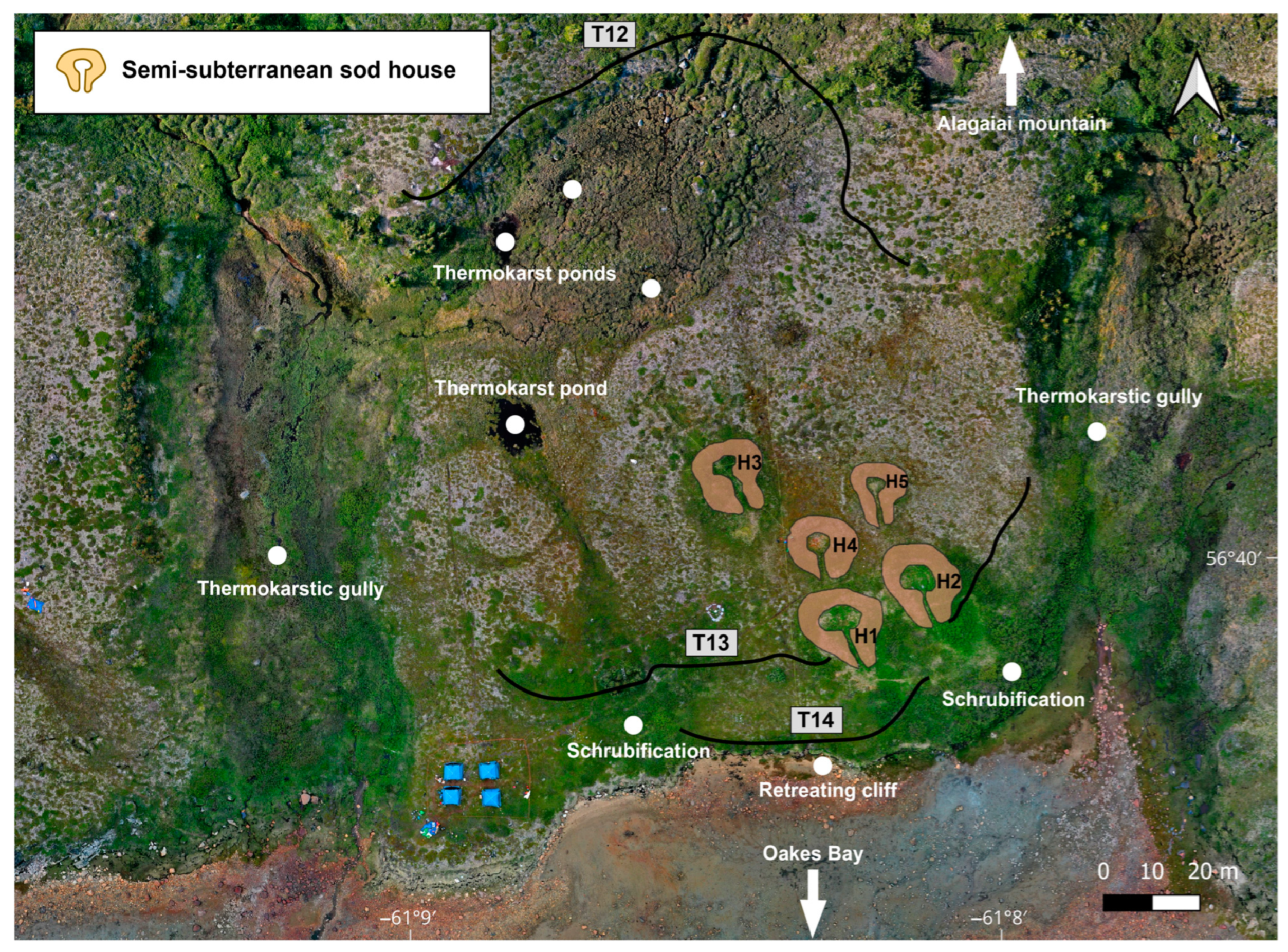
2. Study Site
3. Methods
3.1. Electrical Resistivity Tomography (ERT)
3.2. Ground-Penetrating Radar (GPR)
3.3. Electromagnetic Induction (EMI)
4. Results and Interpretation
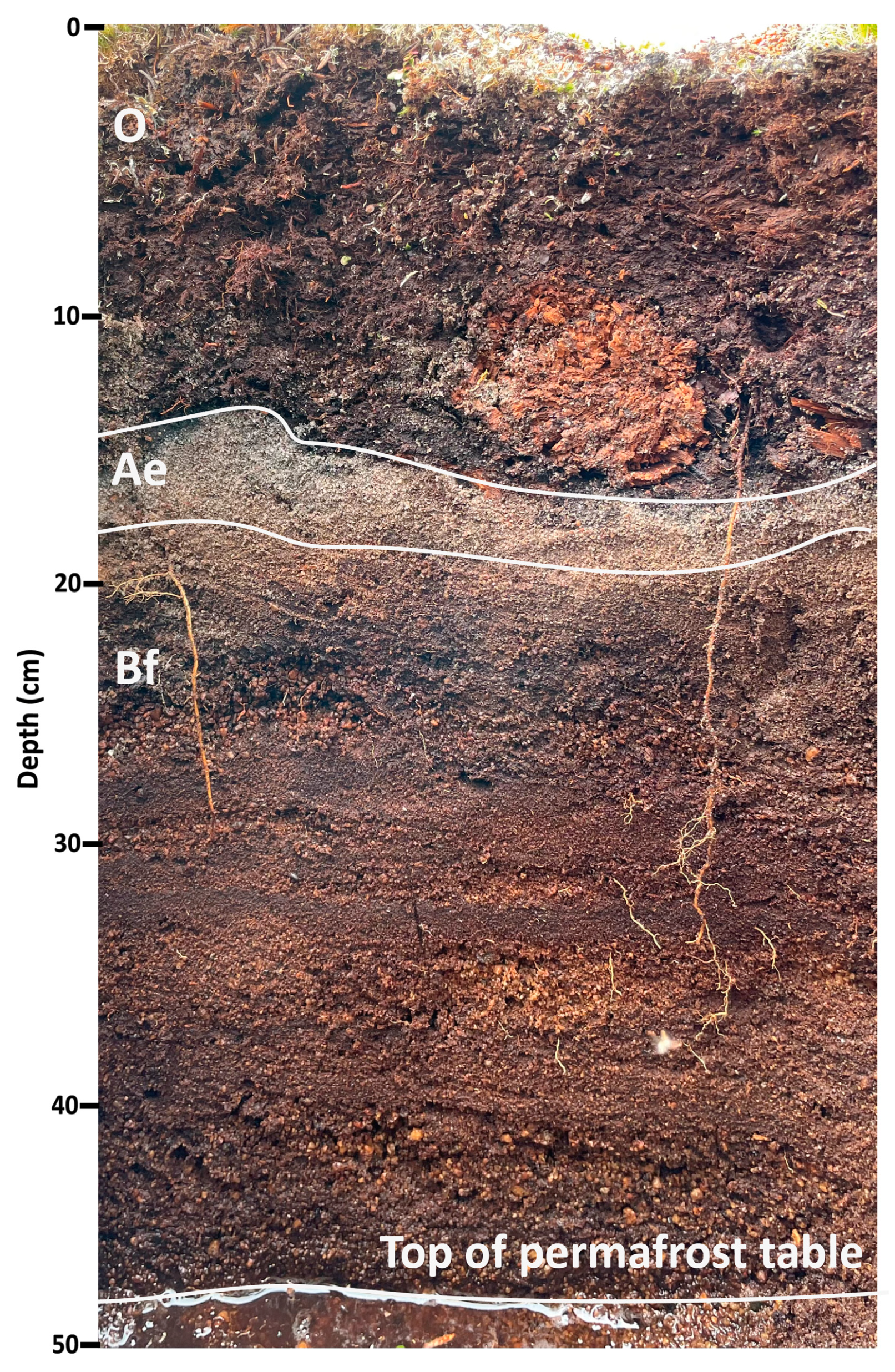
4.1. On-Site Pits and Pedostratigraphy
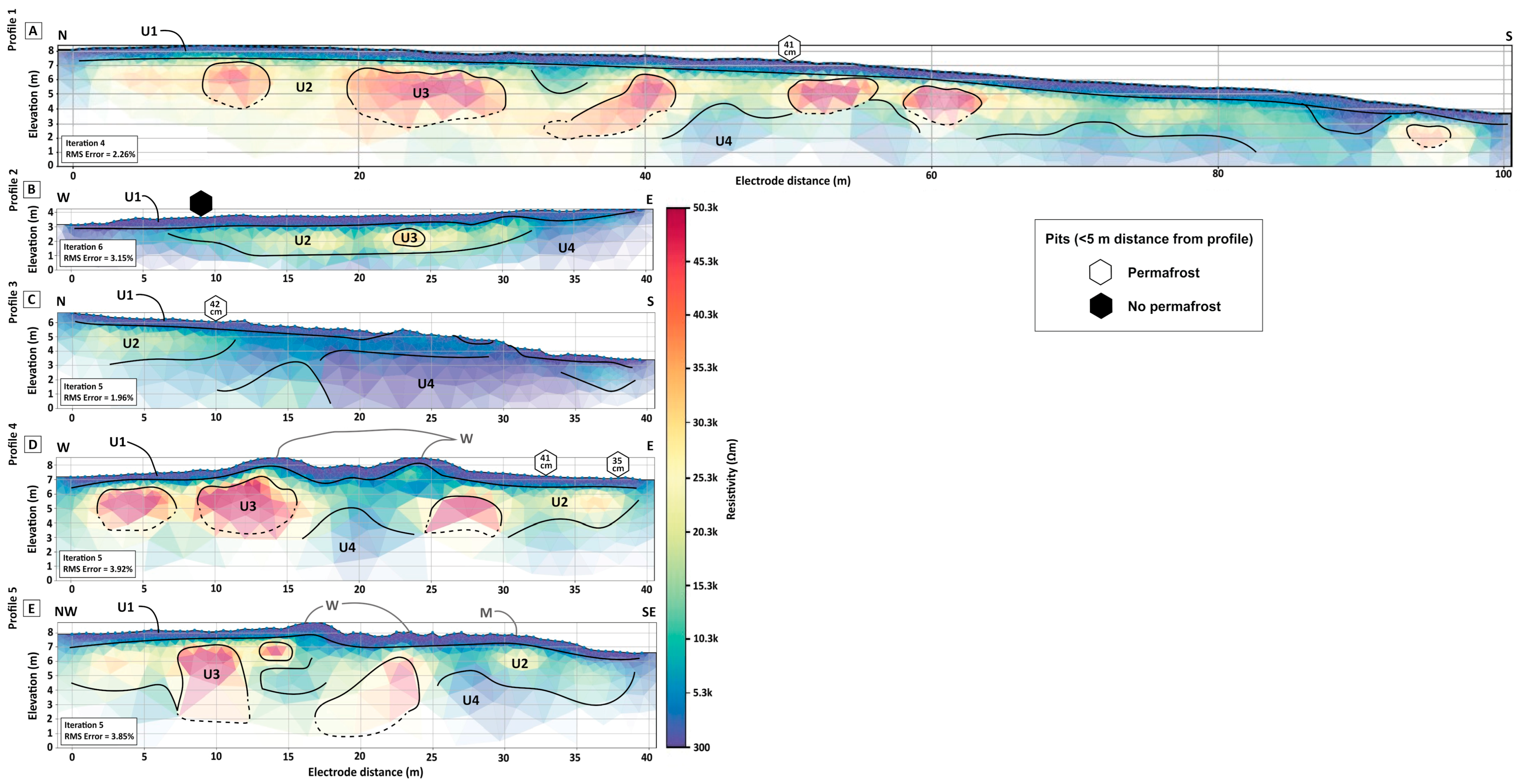
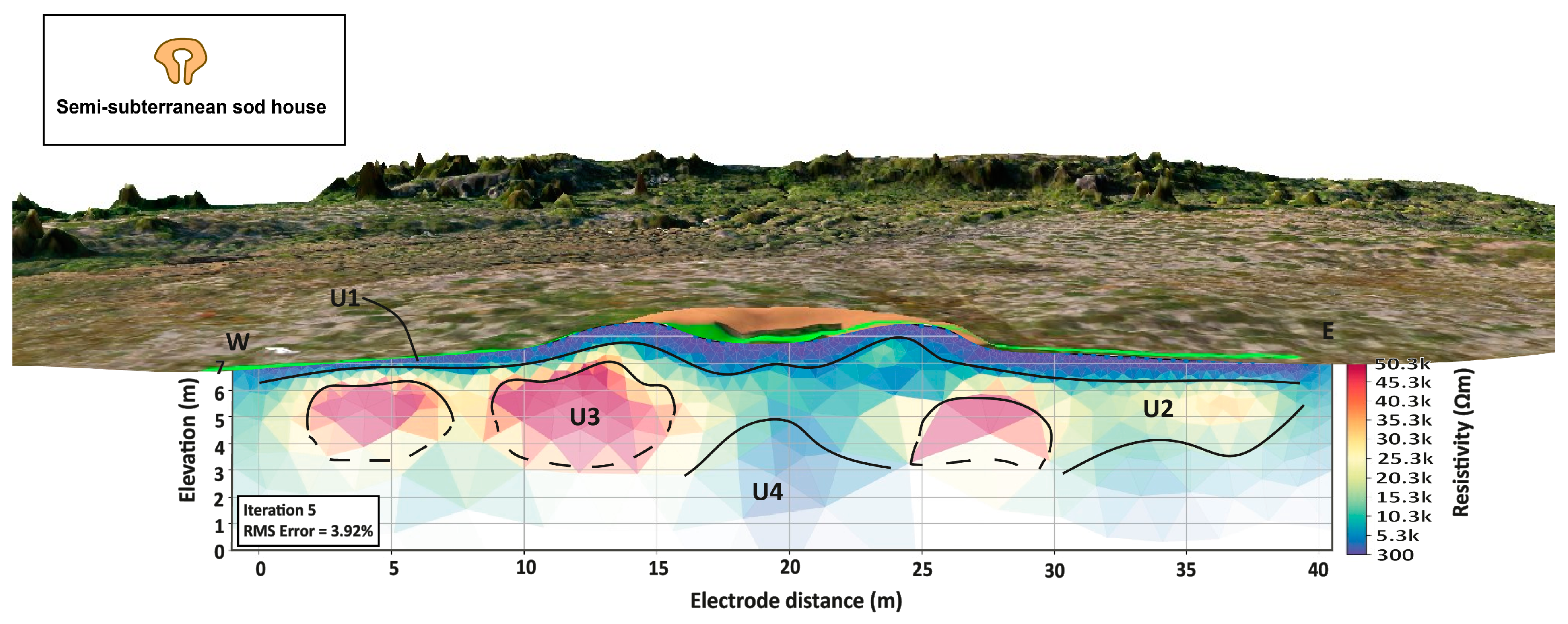
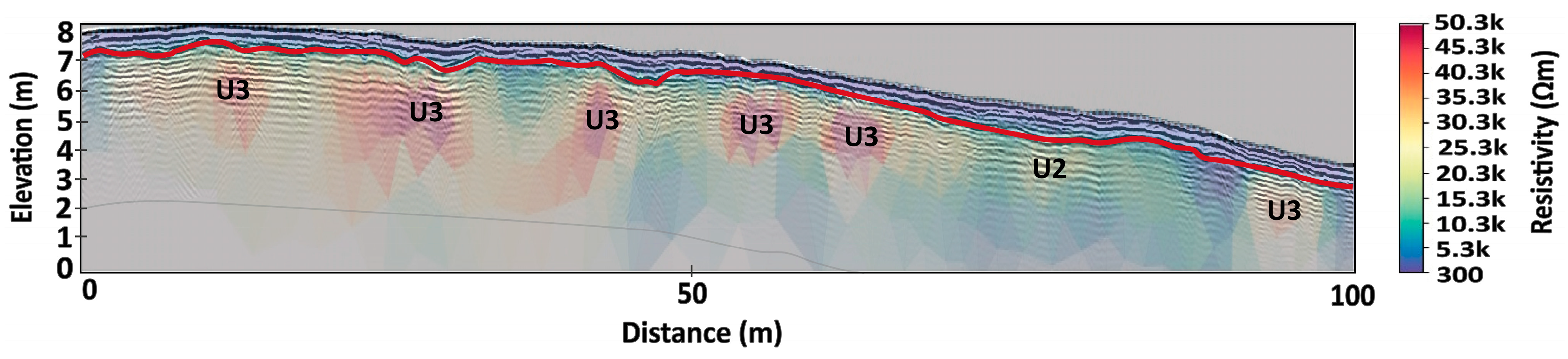
4.2. Electrical Resistivity Tomography (ERT)
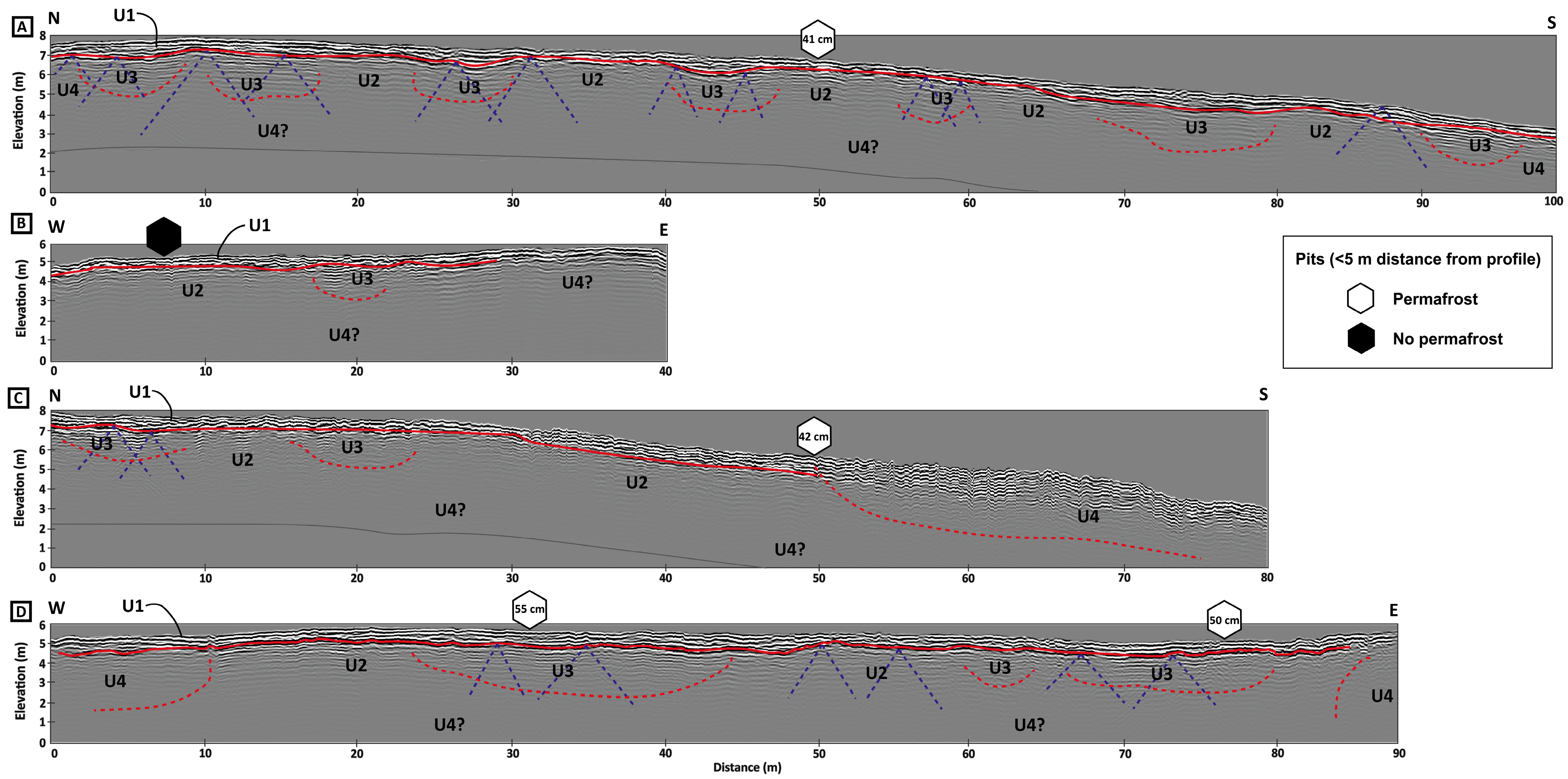
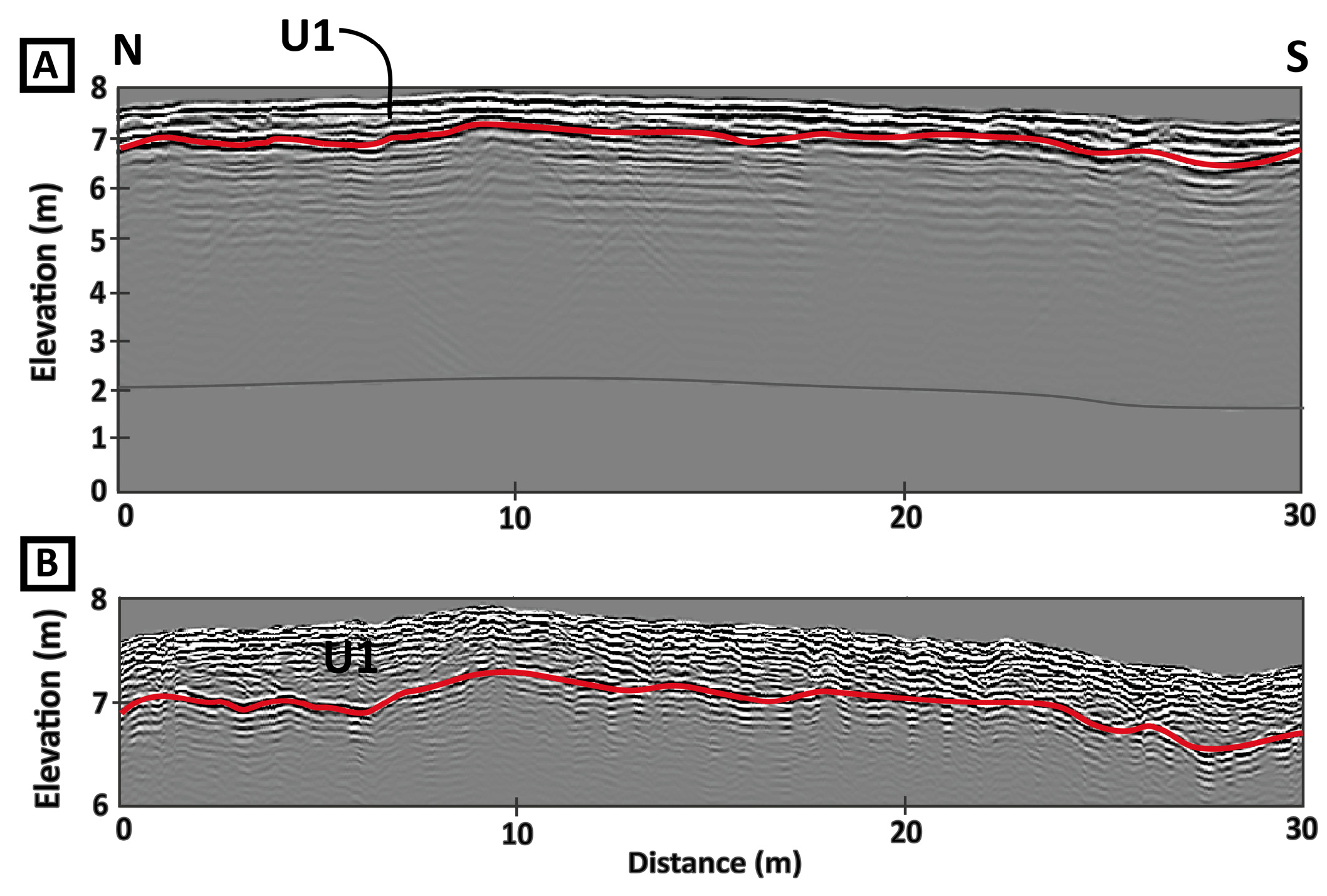
4.3. Ground-Penetrating Radar (GPR)
5. Discussion
5.1. Complementarity of the Geophysical Methods
5.2. Current Distribution of Permafrost at the Site Scale
5.3. Current Distribution of Permafrost within Inuit Semi-Subterranean Sod Houses
5.4. Anticipated Evolution of Permafrost at Oakes Bay 1
6. Conclusions
Supplementary Materials
Author Contributions
Funding
Data Availability Statement
Acknowledgments
Conflicts of Interest
References
- Wilson, S. AMAP Assessment 2016: Chemicals of Emerging Arctic Concern; Arctic Monitoring and Assessment Programme (AMAP): Oslo, Norway, 2017; ISBN 978-82-7971-104-9. [Google Scholar]
- Hassol, S.J. Impacts of a Warming Arctic: Arctic Climate Impact Assessment; Cambridge University Press: Cambridge, UK, 2004; ISBN 978-0-521-61778-9. [Google Scholar]
- Hollesen, J.; Callanan, M.; Dawson, T.; Fenger-Nielsen, R.; Friesen, T.M.; Jensen, A.M.; Markham, A.; Martens, V.V.; Pitulko, V.V.; Rockman, M. Climate Change and the Deteriorating Archaeological and Environmental Archives of the Arctic. Antiquity 2018, 92, 573–586. [Google Scholar] [CrossRef]
- Nicu, I.C.; Fatorić, S. Climate Change Impacts on Immovable Cultural Heritage in Polar Regions: A Systematic Bibliometric Review. WIREs Clim. Chang. 2023, 14, e822. [Google Scholar] [CrossRef]
- Friesen, T.M. The Arctic CHAR Project: Climate Change Impacts on the Inuvialuit Archaeological Record. Nouv. Archéologie 2015, 141, 31–37. [Google Scholar] [CrossRef]
- Lantuit, H.; Pollard, W.H. Fifty Years of Coastal Erosion and Retrogressive Thaw Slump Activity on Herschel Island, Southern Beaufort Sea, Yukon Territory, Canada. Geomorphology 2008, 95, 84–102. [Google Scholar] [CrossRef]
- O’Rourke, M.J.E. Archaeological Site Vulnerability Modelling: The Influence of High Impact Storm Events on Models of Shoreline Erosion in the Western Canadian Arctic. Open Archaeol. 2017, 3, 1–16. [Google Scholar] [CrossRef]
- Way, R.G.; Lewkowicz, A.G.; Zhang, Y. Characteristics and Fate of Isolated Permafrost Patches in Coastal Labrador, Canada. Cryosphere 2018, 12, 2667–2688. [Google Scholar] [CrossRef]
- Tape, K.; Sturm, M.; Racine, C. The Evidence for Shrub Expansion in Northern Alaska and the Pan-Arctic. Glob. Chang. Biol. 2006, 12, 686–702. [Google Scholar] [CrossRef]
- Myers-Smith, I.H.; Forbes, B.C.; Wilmking, M.; Hallinger, M.; Lantz, T.; Blok, D.; Tape, K.D.; Macias-Fauria, M.; Sass-Klaassen, U.; Lévesque, E.; et al. Shrub Expansion in Tundra Ecosystems: Dynamics, Impacts and Research Priorities. Environ. Res. Lett. 2011, 6, 045509. [Google Scholar] [CrossRef]
- Fenger-Nielsen, R.; Elberling, B.; Kroon, A.; Westergaard-Nielsen, A.; Matthiesen, H.; Harmsen, H.; Madsen, C.K.; Stendel, M.; Hollesen, J. Arctic Archaeological Sites Threatened by Climate Change: A Regional Multi-threat Assessment of Sites in South-west Greenland. Archaeometry 2020, 62, 1280–1297. [Google Scholar] [CrossRef]
- Conyers, L.B. Ground-Penetrating Radar for Geoarchaeology; John Wiley & Sons Inc: Hoboken, NJ, USA, 2016; ISBN 978-1-118-95000-5. [Google Scholar]
- Siart, C.; Forbriger, M.; Bubenzer, O. Digital Geoarchaeology: New Techniques for Interdisciplinary Human-Environmental Research; Natural Science in Archaeology; Springer International Publishing: Cham, Switzerland, 2018; ISBN 978-3-319-25314-5. [Google Scholar]
- Kneisel, C.; Hauck, C.; Fortier, R.; Moorman, B. Advances in Geophysical Methods for Permafrost Investigations. Permafr. Periglac. Process. 2008, 19, 157–178. [Google Scholar] [CrossRef]
- Hubbard, S.S.; Gangodagamage, C.; Dafflon, B.; Wainwright, H.; Peterson, J.; Gusmeroli, A.; Ulrich, C.; Wu, Y.; Wilson, C.; Rowland, J.; et al. Quantifying and Relating Land-Surface and Subsurface Variability in Permafrost Environments Using LiDAR and Surface Geophysical Datasets. Hydrogeol. J. 2013, 21, 149–169. [Google Scholar] [CrossRef]
- Sjöberg, Y.; Marklund, P.; Pettersson, R.; Lyon, S.W. Geophysical Mapping of Palsa Peatland Permafrost. Cryosphere 2015, 9, 465–478. [Google Scholar] [CrossRef]
- Saintenoy, A.; Pessel, M.; Grenier, C.; Léger, E.; Danilov, K.; Bazhin, K.; Khristoforov, I.; Séjourné, A.; Konstantinov, P. Coupling GPR and ERT Data Interpretation to Study the Thermal Imprint of a River in Syrdakh (Central Yakutia, Russia). In Proceedings of the 18th International Conference on Ground Penetrating Radar, Golden, CO, USA, 14–19 June 2020; Society of Exploration Geophysicists: Golden, CO, USA, 2020; pp. 93–96. [Google Scholar]
- Bussière, L.; Schmutz, M.; Fortier, R.; Lemieux, J.; Dupuy, A. Near-surface Geophysical Imaging of a Thermokarst Pond in the Discontinuous Permafrost Zone in Nunavik (Québec), Canada. Permafr. Periglac. Process. 2022, 33, 353–369. [Google Scholar] [CrossRef]
- Modin, I.N.; Arzhantseva, I.A.; Andreyev, M.A.; Akulenko, S.A.; Kats, M.Y. Geophysical Investigations on Por-Bajin Island in the Republic of Tuva. Mosc. Univ. Geol. Bull. 2010, 65, 428–433. [Google Scholar] [CrossRef]
- Wolff, C.B.; Urban, T.M. Geophysical Analysis at the Old Whaling Site, Cape Krusenstern, Alaska, Reveals the Possible Impact of Permafrost Loss on Archaeological Interpretation. Polar Res. 2013, 32, 19888. [Google Scholar] [CrossRef]
- Hodgetts, L.; Dawson, P.; Eastaugh, E. Archaeological Magnetometry in an Arctic Setting: A Case Study from Maguse Lake, Nunavut. J. Archaeol. Sci. 2011, 38, 1754–1762. [Google Scholar] [CrossRef]
- Landry, D.B.; Ferguson, I.J.; Milne, S.B.; Park, R.W. Combined Geophysical Approach in a Complex Arctic Archaeological Environment: A Case Study from the LdFa-1 Site, Southern Baffin Island, Nunavut. Archaeol. Prospect. 2015, 22, 157–170. [Google Scholar] [CrossRef]
- Hodgetts, L.M.; Eastaugh, E.J.H. The Role of Magnetometry in Managing Arctic Archaeological Sites in the Face of Climate Change. Adv. Archaeol. Pract. 2017, 5, 110–124. [Google Scholar] [CrossRef]
- Way, R.G.; Viau, A.E. Natural and Forced Air Temperature Variability in the Labrador Region of Canada during the Past Century. Theor. Appl. Climatol. 2015, 121, 413–424. [Google Scholar] [CrossRef]
- Barrette, C.; Brown, R.; Way, R.; Mailhot, A.; Émilia, P.; Diaconescu, P.; Grenier, D.; Chaumont, D.; Dumont, C.; Sévigny, S.; et al. Chapter 2: Nunavik and Nunatsiavut regional climate information update. In Nunavik and Nunatsiavut: From Science to Policy, an Integrated Regional Impact Study (IRIS) of Climate Change and Modernization, Second Iteration; Ropars, P., Allard, M., LeMay, M., Eds.; ArcticNet Inc.: Québec, QC, Canada, 2020. [Google Scholar]
- Woollett, J. Oakes Bay 1: A Preliminary Reconstruction of a Labrador Inuit Seal Hunting Economy in the Context of Climate Change. Geogr. Tidsskr.-Dan. J. Geogr. 2010, 110, 245–259. [Google Scholar] [CrossRef]
- Roy, N.; Bhiry, N.; Woollett, J. Environmental Change and Terrestrial Resource Use by the T Hule and I Nuit of L Abrador, C Anada. Geoarchaeology 2012, 27, 18–33. [Google Scholar] [CrossRef]
- Couture, A.; Bhiry, N.; Monette, Y.; Woollett, J. A Geochemical Analysis of 18th-Century Inuit Communal House Floors in Northern Labrador. J. Archaeol. Sci. Rep. 2016, 6, 71–81. [Google Scholar] [CrossRef]
- Foury, Y.; Bhiry, N.; Woollett, J.; Bhiry, N.; Woollett, J. L’occupation du Site Hivernal Inuit Oakes Bay 1 (HeCg-08), Labrador, Canada: Micromorphologie et Zooarchéologie des Dépotoirs; Université Laval: Québec, QC, Canada, 2017. [Google Scholar]
- Marko, J.R.; Fissel, D.B.; Wadhams, P.; Kelly, P.M.; Brown, R.D. Iceberg Severity off Eastern North America: Its Relationship to Sea Ice Variability and Climate Change. J. Clim. 1994, 7, 1335–1351. [Google Scholar] [CrossRef]
- Données Climatiques Historiques. Available online: https://climat.meteo.gc.ca/ (accessed on 20 December 2023).
- Ouellet-Bernier, M.-M.; De Vernal, A.; Chartier, D.; Boucher, É. Historical Perspectives on Exceptional Climatic Years at the Labrador/Nunatsiavut Coast 1780 to 1950. Quat. Res. 2021, 101, 114–128. [Google Scholar] [CrossRef]
- Wardle, R.J.; Gower, C.F.; Ryan, B.; Nunn, G.A.G.; James, D.T.; Kerr, A. Geological Map of Labrador; 1:1 Million Scale; Geological Survey, Map 97-07; Government of Newfoundland and Labrador, Department of Mines and Energy: Labrador, NL, Canada, 1997.
- Margold, M.; Stokes, C.R.; Clark, C.D. Reconciling Records of Ice Streaming and Ice Margin Retreat to Produce a Palaeogeographic Reconstruction of the Deglaciation of the Laurentide Ice Sheet. Quat. Sci. Rev. 2018, 189, 1–30. [Google Scholar] [CrossRef]
- Clark, P.U.; Fitzhugh, W.W. Late Deglaciation of the Central Labrador Coast and Its Implications for the Age of Glacial Lakes Naskaupi and McLean and for Prehistory. Quat. Res. 1990, 34, 296–305. [Google Scholar] [CrossRef]
- Roy, N.; Woollett, J.; Bhiry, N.; Lemus-Lauzon, I.; Delwaide, A.; Marguerie, D. Anthropogenic and Climate Impacts on Subarctic Forests in the Nain Region, Nunatsiavut: Dendroecological and Historical Approaches. Écoscience 2021, 28, 361–376. [Google Scholar] [CrossRef]
- Oblogov, G.E.; Vasiliev, A.A.; Streletskiy, D.A.; Shiklomanov, N.I.; Nyland, K.E. Localized Vegetation, Soil Moisture, and Ice Content Offset Permafrost Degradation under Climate Warming. Geosciences 2023, 13, 129. [Google Scholar] [CrossRef]
- Guth, P.L.; Van Niekerk, A.; Grohmann, C.H.; Muller, J.-P.; Hawker, L.; Florinsky, I.V.; Gesch, D.; Reuter, H.I.; Herrera-Cruz, V.; Riazanoff, S.; et al. Digital Elevation Models: Terminology and Definitions. Remote Sens. 2021, 13, 3581. [Google Scholar] [CrossRef]
- Dahlin, T.; Zhou, B. A Numerical Comparison of 2D Resistivity Imaging with 10 Electrode Arrays. Geophys. Prospect. 2004, 52, 379–398. [Google Scholar] [CrossRef]
- Rücker, C.; Günther, T.; Wagner, F.M. pyGIMLi: An Open-Source Library for Modelling and Inversion in Geophysics. Comput. Geosci. 2017, 109, 106–123. [Google Scholar] [CrossRef]
- Marescot, L.; Loke, M.H.; Chapellier, D.; Delaloye, R.; Lambiel, C.; Reynard, E. Assessing Reliability of 2D Resistivity Imaging in Mountain Permafrost Studies Using the Depth of Investigation Index Method. Surf. Geophys. 2003, 1, 57–67. [Google Scholar] [CrossRef]
- Supper, R.; Ottowitz, D.; Jochum, B.; Römer, A.; Pfeiler, S.; Kauer, S.; Keuschnig, M.; Ita, A. Geoelectrical Monitoring of Frozen Ground and Permafrost in Alpine Areas: Field Studies and Considerations towards an Improved Measuring Technology. Surf. Geophys. 2014, 12, 93–115. [Google Scholar] [CrossRef]
- Hauck, C.; Kneisel, C. Applied Geophysics in Periglacial Environments, 1st ed.; Cambridge University Press: Cambridge, UK, 2008; ISBN 978-0-521-88966-7. [Google Scholar]
- Halla, C.; Blöthe, J.H.; Tapia Baldis, C.; Trombotto Liaudat, D.; Hilbich, C.; Hauck, C.; Schrott, L. Ice Content and Interannual Water Storage Changes of an Active Rock Glacier in the Dry Andes of Argentina. Cryosphere 2021, 15, 1187–1213. [Google Scholar] [CrossRef]
- You, Y.; Yu, Q.; Pan, X.; Wang, X.; Guo, L. Application of Electrical Resistivity Tomography in Investigating Depth of Permafrost Base and Permafrost Structure in Tibetan Plateau. Cold Reg. Sci. Technol. 2013, 87, 19–26. [Google Scholar] [CrossRef]
- Douglas, T.A.; Jorgenson, M.T.; Brown, D.R.N.; Campbell, S.W.; Hiemstra, C.A.; Saari, S.P.; Bjella, K.; Liljedahl, A.K. Degrading Permafrost Mapped with Electrical Resistivity Tomography, Airborne Imagery and LiDAR, and Seasonal Thaw Measurements. Geophysics 2016, 81, WA71–WA85. [Google Scholar] [CrossRef]
- Urruela, A.; Rivero, L.; Casas, A.; Garcia-Artigas, R.; Sendrós, A.; Lovera, R.; Himi, M. Improving the Resolution of Investigation Using ERT Instruments with a Reduced Number of Electrodes. J. Appl. Geophys. 2021, 186, 104239. [Google Scholar] [CrossRef]
- Everett, M.E. Near-Surface Applied Geophysics, 1st ed.; Cambridge University Press: Cambridge, UK, 2013; ISBN 978-1-107-01877-8. [Google Scholar]
- Martinez, A.; Byrnes, A.P. Modeling Dielectric-Constant Values of Geologic Materials: An Aid to Ground-Penetrating Radar Data Collection and Interpretation. Curr. Res. Earth Sci. 2001, 247, 1–16. [Google Scholar] [CrossRef]
- Sandmeier, K.J. Reflexw-Program for the Processing of Seismic, Acoustic or Electromagnetic Reflection, Refraction and Transmission Data, (version 9.5.7). Windows; Sandmeier Geophysical Research: Karlsruhe, Gremany, 2020. [Google Scholar]
- Campbell, S.; Affleck, R.T.; Sinclair, S. Ground-Penetrating Radar Studies of Permafrost, Periglacial, and near-Surface Geology at McMurdo Station, Antarctica. Cold Reg. Sci. Technol. 2018, 148, 38–49. [Google Scholar] [CrossRef]
- Davis, J.L.; Annan, A.P. Ground-Penetrating Radar for High-Resolution Mapping of Soil and Rock Stratigraphy 1. Geophys. Prospect. 1989, 37, 531–551. [Google Scholar] [CrossRef]
- De Pascale, G.P.; Pollard, W.H.; Williams, K.K. Geophysical Mapping of Ground Ice Using a Combination of Capacitive Coupled Resistivity and Ground-penetrating Radar, Northwest Territories, Canada. J. Geophys. Res. Earth Surf. 2008, 113, 2006JF000585. [Google Scholar] [CrossRef]
- Angelopoulos, M.C.; Pollard, W.H.; Couture, N.J. The Application of CCR and GPR to Characterize Ground Ice Conditions at Parsons Lake, Northwest Territories. Cold Reg. Sci. Technol. 2013, 85, 22–33. [Google Scholar] [CrossRef]
- Hilbich, C.; Marescot, L.; Hauck, C.; Loke, M.H.; Mäusbacher, R. Applicability of Electrical Resistivity Tomography Monitoring to Coarse Blocky and Ice-rich Permafrost Landforms. Permafr. Periglac. Process. 2009, 20, 269–284. [Google Scholar] [CrossRef]
- Harris, S.A.; French, H.M.; Heginbottom, J.A.; Johnston, G.H.; Ladanyi, B.; Sego, D.C.; van Everdingen, R.O. Glossary of Permafrost and Related Ground-Ice Terms; National Research Council of Canada. Associate Committee on Geotechnical Research; Permafrost Subcommittee: Ottawa, ON, Canada, 1988; 159p. [Google Scholar]
- Lewkowicz, A.G.; Etzelmüller, B.; Smith, S.L. Characteristics of Discontinuous Permafrost Based on Ground Temperature Measurements and Electrical Resistivity Tomography, Southern Yukon, Canada. Permafr. Periglac. Process. 2011, 22, 320–342. [Google Scholar] [CrossRef]
- Forte, E.; French, H.M.; Raffi, R.; Santin, I.; Guglielmin, M. Investigations of Polygonal Patterned Ground in Continuous Antarctic Permafrost by Means of Ground Penetrating Radar and Electrical Resistivity Tomography: Some Unexpected Correlations. Permafr. Periglac. Process. 2022, 33, 226–240. [Google Scholar] [CrossRef]
- Gusmeroli, A.; Liu, L.; Schaefer, K.; Zhang, T.; Schaefer, T.; Grosse, G. Active Layer Stratigraphy and Organic Layer Thickness at a Thermokarst Site in Arctic Alaska Identified Using Ground Penetrating Radar. Arct. Antarct. Alp. Res. 2015, 47, 195–202. [Google Scholar] [CrossRef]
- Moorman, B.J.; Robinson, S.D.; Burgess, M.M. Imaging Periglacial Conditions with Ground-penetrating Radar. Permafr. Periglac. Process. 2003, 14, 319–329. [Google Scholar] [CrossRef]
- Onaca, A.; Ardelean, F.; Ardelean, A.; Magori, B.; Sîrbu, F.; Voiculescu, M.; Gachev, E. Assessment of Permafrost Conditions in the Highest Mountains of the Balkan Peninsula. CATENA 2020, 185, 104288. [Google Scholar] [CrossRef]
- Arcone, S.A.; Lawson, D.E.; Delaney, A.J.; Strasser, J.C.; Strasser, J.D. Ground-penetratinng Radar Reflection Profiling of Groundwater and Bedrock in an Area of Discontinuous Permafrost. Geophysics 1998, 63, 1573–1584. [Google Scholar] [CrossRef]
- Watanabe, T.; Matsuoka, N.; Christiansen, H.H. Ice- and Soil-Wedge Dynamics in the Kapp Linné Area, Svalbard, Investigated by Two- and Three-Dimensional GPR and Ground Thermal and Acceleration Regimes. Permafr. Periglac. Process. 2013, 24, 39–55. [Google Scholar] [CrossRef]
- Leger, E.; Dafflon, B.; Soom, F.; Peterson, J.; Ulrich, C.; Hubbard, S. Quantification of Arctic Soil and Permafrost Properties Using Ground-Penetrating Radar and Electrical Resistivity Tomography Datasets. IEEE J. Sel. Top. Appl. Earth Obs. Remote Sens. 2017, 10, 4348–4359. [Google Scholar] [CrossRef]
- Bode, J.; Moorman, B.; Stevens, C.; Solomon, S. Estimation of Ice Wedge Volume in the Big Lake Area, Mackenzie Delta, NWT, Canada. In Proceedings of the 9th International Conference on Permafrost, Fairbanks, AK, USA, 29 June–3 July 2008. [Google Scholar]
- Yoshikawa, K.; Leuschen, C.; Ikeda, A.; Harada, K.; Gogineni, P.; Hoekstra, P.; Hinzman, L.; Sawada, Y.; Matsuoka, N. Comparison of Geophysical Investigations for Detection of Massive Ground Ice (Pingo Ice). J. Geophys. Res. Planets 2006, 111, 2005JE002573. [Google Scholar] [CrossRef]
- Bouchard, F.; Francus, P.; Pienitz, R.; Laurion, I.; Feyte, S. Subarctic Thermokarst Ponds: Investigating Recent Landscape Evolution and Sediment Dynamics in Thawed Permafrost of Northern Québec (Canada). Arct. Antarct. Alp. Res. 2014, 46, 251–271. [Google Scholar] [CrossRef]
- Anderson, D.; Ford, J.D.; Way, R.G. The Impacts of Climate and Social Changes on Cloudberry (Bakeapple) Picking: A Case Study from Southeastern Labrador. Hum. Ecol. 2018, 46, 849–863. [Google Scholar] [CrossRef] [PubMed]
- Davis, E.; Trant, A.; Hermanutz, L.; Way, R.G.; Lewkowicz, A.G.; Siegwart Collier, L.; Cuerrier, A.; Whitaker, D. Plant–Environment Interactions in the Low Arctic Torngat Mountains of Labrador. Ecosystems 2021, 24, 1038–1058. [Google Scholar] [CrossRef]
- Wang, Y.; Way, R.G.; Beer, J.; Forget, A.; Tutton, R.; Purcell, M.C. Significant Underestimation of Peatland Permafrost along the Labrador Sea Coastline in Northern Canada. Cryosphere 2023, 17, 63–78. [Google Scholar] [CrossRef]
- Way, R.; Lewkowicz, A.; Wang, Y.; McCarney, P. Permafrost Investigations Below The Marine Limit At Nain, Nunatsiavut, Canada. In Proceedings of the Regional Conference on Permafrost 2021 and the 19th International Conference on Cold Regions Engineering, Reston, VA, USA, 24–29 October 2021. [Google Scholar] [CrossRef]
- French, H.M. The Periglacial Environment, 4th ed.; Wiley, Blackwell: Hoboken, NJ, USA, 2017; ISBN 978-1-119-13281-3. [Google Scholar]
- Connon, R.; Devoie, É.; Hayashi, M.; Veness, T.; Quinton, W. The Influence of Shallow Taliks on Permafrost Thaw and Active Layer Dynamics in Subarctic Canada. J. Geophys. Res. Earth Surf. 2018, 123, 281–297. [Google Scholar] [CrossRef]
- Devoie, É.G.; Craig, J.R.; Dominico, M.; Carpino, O.; Connon, R.F.; Rudy, A.C.A.; Quinton, W.L. Mechanisms of Discontinuous Permafrost Thaw in Peatlands. J. Geophys. Res. Earth Surf. 2021, 126, e2021JF006204. [Google Scholar] [CrossRef]
- Kasprzak, M. Seawater Intrusion on the Arctic Coast (Svalbard): The Concept of Onshore-Permafrost Wedge. Geosciences 2020, 10, 349. [Google Scholar] [CrossRef]
- Dobiński, W.; Kasprzak, M. Permafrost Base Degradation: Characteristics and Unknown Thread With Specific Example From Hornsund, Svalbard. Front. Earth Sci. 2022, 10, 802157. [Google Scholar] [CrossRef]
- Smith, S.L.; O’Neill, H.B.; Isaksen, K.; Noetzli, J.; Romanovsky, V.E. The Changing Thermal State of Permafrost. Nat. Rev. Earth Environ. 2022, 3, 10–23. [Google Scholar] [CrossRef]
- Production de la 2e Approximation de la Carte de Pergélisol du Québec en Fonction des Paramètres Géomorphologiques, Écologiques, et des Processus Physiques Liés au Climat. Available online: https://mffp.gouv.qc.ca/nos-publications/production-2e-approximation-carte-pergelisol-quebec/ (accessed on 14 December 2023).
- Martin, L.; Nitzbon, J.; Aas, K.; Etzelmüller, B.; Kristiansen, H.; Westermann, S. Stability Conditions of Peat Plateaus and Palsas in Northern Norway. J. Geophys. Res. Earth Surf. 2019, 124, 705–719. [Google Scholar] [CrossRef]
- Shur, Y.L.; Jorgenson, M.T. Patterns of Permafrost Formation and Degradation in Relation to Climate and Ecosystems. Permafr. Periglac. Process. 2007, 18, 7–19. [Google Scholar] [CrossRef]
- Spence, C.; Norris, M.; Bickerton, G.; Bonsal, B.R.; Brua, R.; Culp, J.M.; Dibike, Y.; Gruber, S.; Morse, P.D.; Peters, D.L.; et al. The Canadian Water Resource Vulnerability Index to Permafrost Thaw (CWRVI PT). Arct. Sci. 2020, 6, 437–462. [Google Scholar] [CrossRef]
- Wright, S.N.; Thompson, L.M.; Olefeldt, D.; Connon, R.F.; Carpino, O.A.; Beel, C.R.; Quinton, W.L. Thaw-Induced Impacts on Land and Water in Discontinuous Permafrost: A Review of the Taiga Plains and Taiga Shield, Northwestern Canada. Earth-Sci. Rev. 2022, 232, 104104. [Google Scholar] [CrossRef]
- Guimond, J.A.; Mohammed, A.A.; Walvoord, M.A.; Bense, V.F.; Kurylyk, B.L. Saltwater Intrusion Intensifies Coastal Permafrost Thaw. Geophys. Res. Lett. 2021, 48, e2021GL094776. [Google Scholar] [CrossRef]
- Porada, P.; Ekici, A.; Beer, C. Effects of Bryophyte and Lichen Cover on Permafrost Soil Temperature at Large Scale. Cryosphere 2016, 10, 2291–2315. [Google Scholar] [CrossRef]
- Tjelldén, A.K.E.; Kristiansen, S.M.; Matthiesen, H.; Pedersen, O. Impact of Roots and Rhizomes on Wetland Archaeology: A Review. Conserv. Manag. Archaeol. Sites 2015, 17, 370–391. [Google Scholar] [CrossRef]
- Dawson, T.; Hambly, J.; Kelley, A.; Lees, W.; Miller, S. Coastal Heritage, Global Climate Change, Public Engagement, and Citizen Science. Proc. Natl. Acad. Sci. USA 2020, 117, 8280–8286. [Google Scholar] [CrossRef]


| Unit | Description | ERT Characteristics | GPR Characteristics |
|---|---|---|---|
| U1 | Active layer | 300 Ω·m to 1000 Ω·m | Many linear reflectors underlain by clear interface |
| U2 | Permafrost | Thousands of Ω·m | Unattenuated zone underneath clear interface |
| U3 | Ice-rich permafrost | >25 kΩ·m | Signal multiples |
| U4 | Talik or water table | <1000 Ω·m | Highly attenuated signal |
Disclaimer/Publisher’s Note: The statements, opinions and data contained in all publications are solely those of the individual author(s) and contributor(s) and not of MDPI and/or the editor(s). MDPI and/or the editor(s) disclaim responsibility for any injury to people or property resulting from any ideas, methods, instructions or products referred to in the content. |
© 2024 by the authors. Licensee MDPI, Basel, Switzerland. This article is an open access article distributed under the terms and conditions of the Creative Commons Attribution (CC BY) license (https://creativecommons.org/licenses/by/4.0/).
Share and Cite
Labrie, R.; Bhiry, N.; Todisco, D.; Finco, C.; Couillet, A. Conceptual Model of Permafrost Degradation in an Inuit Archaeological Context (Dog Island, Labrador): A Geophysical Approach. Geosciences 2024, 14, 95. https://doi.org/10.3390/geosciences14040095
Labrie R, Bhiry N, Todisco D, Finco C, Couillet A. Conceptual Model of Permafrost Degradation in an Inuit Archaeological Context (Dog Island, Labrador): A Geophysical Approach. Geosciences. 2024; 14(4):95. https://doi.org/10.3390/geosciences14040095
Chicago/Turabian StyleLabrie, Rachel, Najat Bhiry, Dominique Todisco, Cécile Finco, and Armelle Couillet. 2024. "Conceptual Model of Permafrost Degradation in an Inuit Archaeological Context (Dog Island, Labrador): A Geophysical Approach" Geosciences 14, no. 4: 95. https://doi.org/10.3390/geosciences14040095