Article

Regional Lithological Mapping Using ASTER-TIR Data: Case Study for the Tibetan Plateau and the Surrounding Area

1
Geological Survey of Japan, National Institute of Advanced Industrial Science and Technology, Tsukuba 3058567, Japan
2
Institute of Remote Sensing and Digital Earth, Chinese Academy of Sciences, Beijing 100094, China
*
Author to whom correspondence should be addressed.
Geosciences 2016, 6(3), 39; https://doi.org/10.3390/geosciences6030039
Submission received: 9 May 2016 / Revised: 8 August 2016 / Accepted: 23 August 2016 / Published: 2 September 2016

Abstract

:
The mineralogical indices the Quartz Index (QI), Carbonate Index (CI) and Mafic Index (MI) for ASTER multispectral thermal infrared (TIR) data were applied to various geological materials for regional lithological mapping on the Tibetan Plateau. Many lithological and structural features are not currently well understood in the central Tibetan Plateau, including the distribution of mafic-ultramafic rocks related to the suture zones, the quartzose and carbonate sedimentary rocks accreted to the Eurasian continent, and sulfate layers related to the Tethys and neo-Tethys geological setting. These rock types can now be mapped with the interpretation of the processed ASTER TIR images described in this paper. A methodology is described for the processing of ASTER TIR data applied to a very wide region of the Tibetan Plateau. The geometrical and radiometric performance of the processed images is discussed, and the advantages of using ortho-rectified data are shown. The challenges of using ASTER data with a small footprint in addition to selecting an appropriate subset of scenes are also examined. ASTER scenes possess a narrow swath width when compared to LANDSAT data (60 km vs. 185 km, respectively). Furthermore, the ASTER data archive is vast, consisting of approximately three million images. These details can present an added level of complexity during an image processing workflow. Finally, geological interpretations made on the maps of the indices are compared with prior geological field studies. The results from the investigations suggest that the indices perform well in the classification of quartzose rocks based on the carbonate and mafic mineral content, in addition to the granitic rocks based on the feldspar content.

Graphical Abstract

1. Introduction

Spectroscopic studies of inorganic materials in the thermal infrared (TIR) region (8–12 μm) [1,2] have demonstrated strong absorption features caused by the stretching vibrations of the Si–O bonds in silicate minerals, the major components of the terrestrial surface, whereas the Si–O bonds do not cause any prominent spectral features in the visible and near-infrared (VNIR) region of the spectrum (0.4–2.5 μm) [3]. Studies carried out during the Apollo missions to the Moon in the 1960s confirmed relationships between the TIR spectral features and the geology of the lunar surface composition (e.g., References [4,5]). For example, it was observed that the emissivity minima due to Si–O stretching vibrations (i.e., reststrahlen bands) moved to longer wavelengths as the composition of the target igneous rocks changed from felsic to ultramafic [6].
The airborne and satellite remote sensing systems were developed after the results of the spectroscopic studies shown above. They demonstrated the capability of detecting rock composition, despite the radiometric, spectral and spatial resolutions being much worse when compared to a modern system such as ASTER. For example, an airborne scanner with two detector elements could distinguish quartz sandstone from nonsilicate surface materials [7]. Additionally, the infrared interferometric spectrometer onboard the Nimbus-4 satellite derived a global surface emissivity map at 9 μm, which discovered the significantly low emissivities over arid areas due to quartz, even with a quite low spatial resolution (~100 km) [8].
The airborne Thermal Infrared Multispectral Scanner called TIMS was the first modern thermal infrared remote sensing system with resolutions adequate for geological applications (e.g., References [9,10]). TIMS and similar airborne systems (e.g., Reference [11]) confirmed their capabilities of detecting the systematic shift of the reststrahlen bands in the silicate rocks and minerals.
The Advanced Spaceborne Thermal Emission and Reflection Radiometer (ASTER) sensor developed by the Japanese government was launched onboard Terra, the first of NASA’s Earth Observing System (EOS) series of satellites, in December 1999 [12]. It is composed of three subsystems: (1) the VNIR subsystem observing the visible to near-infrared region (three bands between 0.5 and 0.9 μm, 15 m resolution with a stereoscopic capability for the NIR band); (2) the SWIR subsystem observing the shortwave infrared region (six bands between 1.6 and 2.5 μm, 30 m resolution); and (3) the TIR subsystem observing the thermal infrared region (five bands between 8 and 12 μm, 90 m resolution, NEΔT < 0.3 K at 300 K), respectively. The spatial coverage of an ASTER image at the surface is approximately 60 × 60 km.
The authors have proposed mineralogical indices defined with the ratioing approach of the ASTER data for detecting lithology or mineralogy [13,14,15,16,17]. Especially the Quartz Index (QI), Carbonate Index (CI) and Mafic Index (MI) defined for the ASTER-TIR data are finely analyzed theoretically and practically, and the performance of the indices in extracting geological information is confirmed [14]. Many studies have applied the indices (e.g., References [13,14,15,16,17,18,19]) and other workers have proved the usefulness and the stability of the indices in the local geological case studies (e.g., References [20,21,22,23,24,25,26,27,28,29]). Despite ASTER radiance registered at the sensor data without atmospheric corrections being adopted for the calculation of the indices, the recognized scene dependency is quite weak if the atmospherically well-conditioned data are selected [17].
One of the main goals of this project is the mapping of large-scale structure and lithology. We therefore commenced research for regional-scale mapping covering a wide area with the spectral indices. Considering the relatively narrow spatial coverage of each ASTER data compared to that of LANDSAT, many scenes need to be mosaicked for mapping a wide area. Additionally, the ASTER data archive is vast and constantly expanding due to the collection of data over the past 16 years that ASTER has been in operation. This makes it difficult to locate suitable scenes when mapping a region of interest. To save time and labor, the selection of well-conditioned data, in addition to prioritizing the selected data and calculating the indices and mosaicking the imagery, was followed [30].
In this paper, we present the regional maps of the indices covering the region of the central Tibetan Plateau and the surrounding area, after summarizing the geology of the study area and introducing the methodology of calculating the indices and producing the regional maps. In total, 386 ASTER products are selected from a database of more than 10,000 scenes to produce the regional maps. The characteristics of the indices for typical geological and the other materials and the radiometric and geometrical performances of the produced maps are discussed. Finally, geological interpretations are made in association with the maps.

2. Materials and Methods
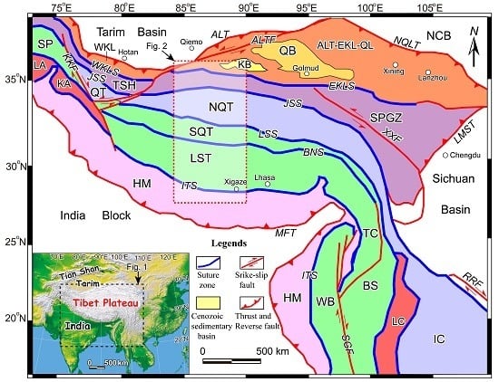
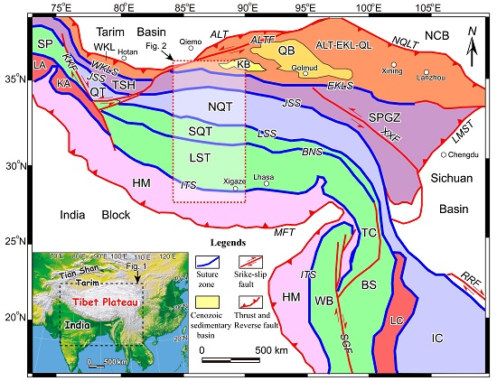
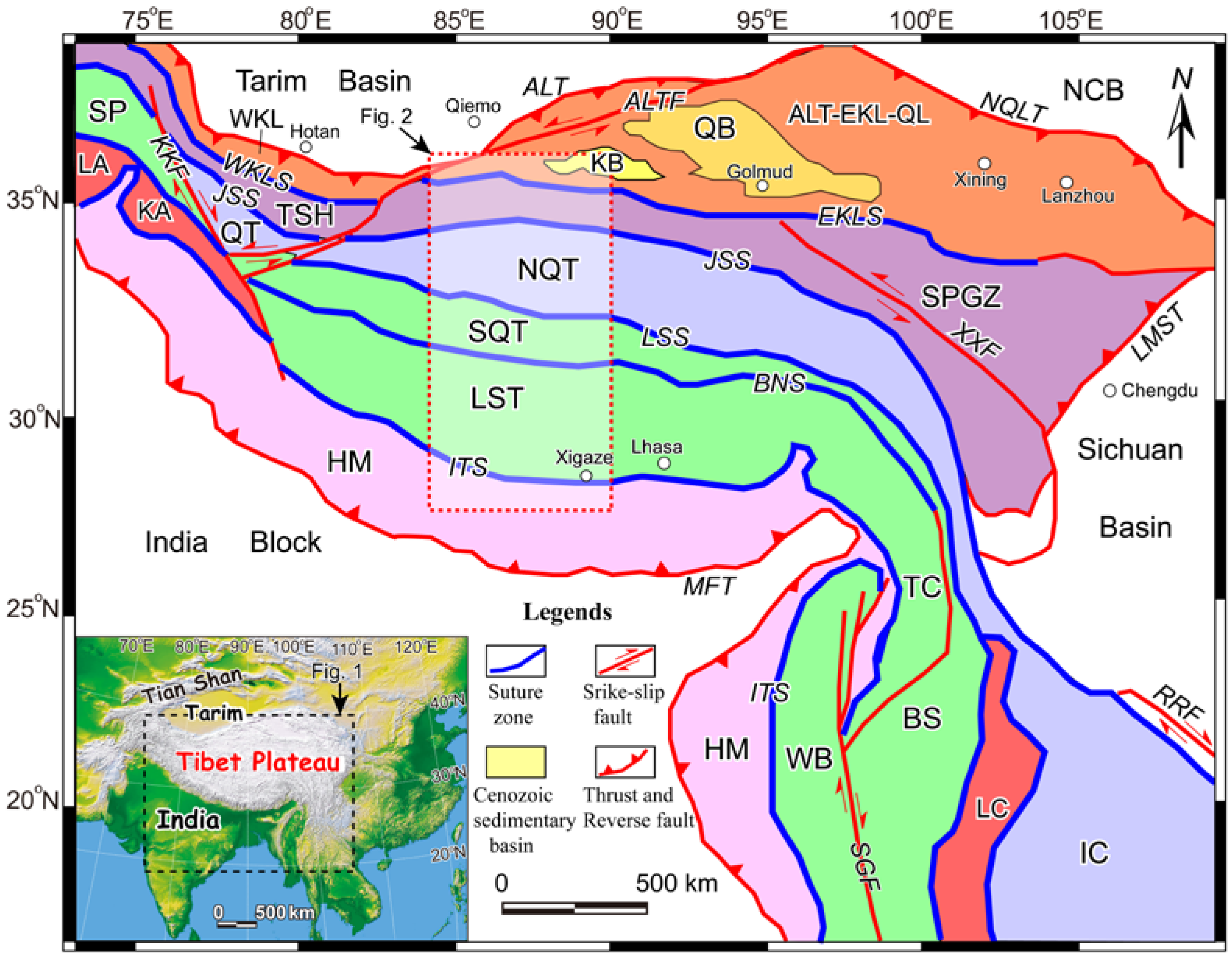
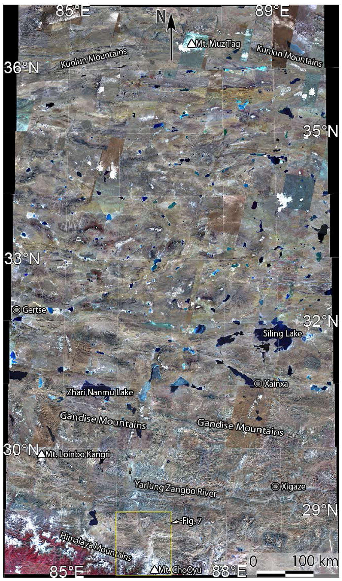
2.1. Study Area

The study area is the central part of the Tibetan Plateau and the surrounding area, bounded by latitude 28° N to 37° N and longitude 84° E to 90° E. The previous studies (e.g., [31,32]) have revealed that the geology of the Tibetan Plateau involves multiple terranes, suture zones containing ophiolites and ophiolitic mélanges, high-P metamorphic belts, magmatic arcs, and accretionary prism complexes that largely developed during the Paleozoic-Mesozoic Eras.
Knowledge of the pre-Cenozoic lithospheric architecture of Tibet is critical for providing initial conditions for models of Tibetan Plateau formation, for establishing strain markers to quantify Cenozoic deformation, and for the development of hypotheses to explain heterogeneous tectonism related to the Cenozoic Indo-Asian collision. From northeast to southwest, Tibet is comprised of the Altyn Tagh–East Kunlun–Qilian, Songpan–Ganzi, Qiangtang, Lhasa and Himalayan terranes, which are separated by east-striking suture zones of Paleozoic to Mesozoic age (Figure 1). Many researchers [31,32] proposed that the formation and evolution of the Tibetan Plateau have been intrinsically related to those of the eastern Tethys, recorded by the Longmu Co-Shuanghu ophiolite mélange zone, the Southern Qiangtang Paleozoic accretionary arc-basin system, the Bangong-Nujiang suture zone, and their associated, composite island arc-basin systems. The present-day Bangong–Shuanghu–Changning–Menglian suture system marks the final closure of the Tethyan Ocean. The Indus-Tsangbo Ocean opened as a back-arc basin in response to the southward subduction of the Tethyan Ocean lithosphere in the Middle Triassic. In addition, it closed as a result of the India-Asia collision at the end of Cretaceous, followed by the northward indention of the Indian plate that resulted in significant intra-continental deformation and plateau uplift in the Cenozoic. Cenozoic deformation mainly produced a crustal scale shear zone and décollement between the Precambrian basement and the cover sequences, regional thrust faults and folds, and strike-slip fault zones.
Figure 1 shows the tectonic setting of the Tibetan Plateau and the surrounding area, modified from the previous studies [33,34,35]. As shown in Figure 1, this study area is composed of the blocks of the Altyn Tagh–East Kunlun–Qilian terrane, Songpan-Ganzi terrane, North Qiangtang terrane, South Qiangtang terrane, Lhasa terrane and Himalayan terrane, from north to south. The most important geological features targeted in this study include the ophiolite belts appearing at the surface along the sutures of the blocks, the quartzose and carbonite sedimentary rocks deposited as the accretionary wedges associated with the subduction of the oceanic plate beneath the continental plate, the granitic rocks intruded with the island arc geological setting, and the distributions of the sulfate layers as the geological evidence of the neo-Tethys environment. The field geological studies so far (e.g., [36,37,38,39,40,41,42,43]) have revealed the distribution of the target lithological features at some limited local areas in the Tibetan Plateau. However, these terranes and suture zones are poorly characterized in central Tibet, with a >1000-km-long and up to 500-km-wide tectonic belt, where the field geological surveys have not yet been accomplished well for most of the region because this area is remote and inaccessible (Figure 1).
The geological map at the scale of 1:1,500,000 is published [44] for the entire Tibetan Plateau region including the study area. Larger-scale geological maps are published at the limited locations, for example the geological map of the ophiolite zone at the scale of 1:200,000 in the middle segment of the Indus-Tsangbo suture zone [45].

2.2. ASTER Data

Since the launch of ASTER in December 1999, the VNIR and TIR subsystems have observed the earth for more than 16 years. This has far exceeded its original lifespan of five years. The SWIR subsystem stopped operation in 2008 due to over saturation and severe striping of the detector. Ownership of the ASTER data had been held by the Ministry of Economy, Trades and Industry (METI) of Japan and NASA, and the ASTER data were distributed by the Japan Space Systems (JSS) and the USGS Eros Data Center, respectively. It was necessary to pay a nominal fee to METI for ordering ASTER data products except for the freely distributed ASTER global digital elevation model (GDEM) products [46] until March 2016. In April 2016, a change in policy was announced [47]. As a result, all ASTER data products are available at no cost. Furthermore, the ASTER data distributor in Japan has changed from JSS to the National Institute of Advanced Industrial Science and Technology (AIST).
The data observed by the ASTER sensors (Level-0 data) are transmitted to ground stations, where the data for each scene is processed to generate the standard Level-1A data product which retains the raw data observed with the sensor. Until March 2016, the ASTER data product was generated and provided as described below. Each standard and semi-standard product of the ASTER data was generated as a Hierarchy Data Format (HDF) file. The standard Level-1B data product was generated automatically for all the Level-1A data satisfying a condition on the detected cloud coverage, as well as based on the user request, which apply the fundamental geometrical and radiometric corrections essential for most of the geoscience applications. Each pixel data in Level-1B is in the measure of radiance registered at the sensor [48,49,50,51]. The standard higher level Level-2B data products of physical parameters including the surface radiance data with the atmospheric corrections on Level-1B data (Level-2B01) [52,53] and the surface emissivity data with the temperature separation processing on the TIR data of the Level-2B01 data (Level-2B04) [54] were generated on the basis of the user request. Also, the semi-standard Level-4 data product of the DEMs was generated from the along-track NIR stereo images (band 3N and 3B) with the downward- and backward-viewing telescopes [55]. The semi-standard Level-3A data product with the ortho-rectification processing had been provided by JSS, which includes the radiance registered at the sensor data equivalent to the one of the Level-1B product and the ASTER-driven DEM [56].
After April 2016, AIST supplies the ortho-rectified data products corresponding to Level-3A in the GeoTIFF files [57], and USGS supplies the data products including the ortho-rectified data of the radiance registered at the sensor (Level-1T) in the HDF files [58] freely to the public covering all over the world, in addition to the ASTER GDEM products already provided to public as described above.
This study uses the ASTER products of radiance at the sensor (e.g., Level-1B, Level-3A). The DN of ASTER-TIR band i in the Level-1B or Level-3A data is linearly related to radiance registered at the sensor (Wm−2·sr−1·µm−1) by [49]
L s e n i = c o e f i × ( D N i 1 ) ,
where coef10 = 0.006882, coef11 = 0.006780, coef12 = 0.006590, coef13 = 0.005693, and coef14 = 0.005225.
Figure 2 shows a false color composite mosaic generated with the ASTER data used in this study annotated with typical geographical information in this study area. All images of the regional maps including Figure 2 are projected using zone 43 of the Universal Transverse Mercator (UTM). As the mosaic VNIR imaging is not the purpose of this study, only an automatic color balancing of the linear stretching in the histogram region covering “average DN ± 3 × σ” was applied, except for the southern part of the study area bounded by latitude 28° N to 30° N, where the color balancing is carefully achieved manually.

2.3. Mineralogical Indices for ASTER-TIR

Based on analysis of the spectral properties for typical terrestrial rocks and minerals shown in Figure 3, the indices, QI, CI and MI were proposed [13]. After the precise analysis on the performance of the indices against the temperature and the atmospheric conditions as well as concerning the separation among the mineral types, the indices were defined [14,17] as described below.
To emphasize the specific spectral feature for quartz in the major rock-forming minerals, e.g., higher emissivity at the 8.6 μm region (corresponding to ASTER band 11) compared to the emissivity at the 8.3 and 9.1 μm regions (corresponding to ASTER band 10 and band 12, respectively) as shown in Figure 3b, QI was defined as [13]
Q I = D 11 × D 11 D 10 × D 12 ,
where Di represents ASTER band i. In this paper, we use radiance data without atmospheric corrections of ASTER Level-1B or Level-3A data. The DN value of each pixel in Level-1B or Level-3A data is linearly converted to radiance registered at the sensor (Wm−2·sr−1·µm−1) with Equation (1). QI is expected to be high for crystallized quartz, and on the other hand, to be low for the common sulfates, typically gypsum because the spectral features for the sulfates in ASTER bands 10 to 12 are the opposite of quartz as recognized in the spectrum of gypsum shown in Figure 3g. Not as strong but similar as the sulfates, K-feldspars and Na-feldspars exhibit the opposite spectral features of quartz. If the rocks are rich in both quartz and feldspar, which often occurs in igneous rock, typically for the granitic rocks, QI is expected to be relatively low [15,17,19,30]. The spectral emissivity property of the rock type shown in Figure 3c supports this expectation. The mixture of quartz and feldspar does not generally occur in sedimentary rocks, which suggests high QI functions well as an indicator of quartz-rich sedimentary rocks. The previous studies have confirmed that high QI is a distinct indicator for quartz-rich sedimentary rocks [14,15,16,17,18,19,21,22,23,26,29,30], and low QI is a distinct indicator primarily of sulfate minerals [15,16,17,30] and secondarily of feldspar-rich silicate rocks [15,17,19,30].
The spectral emissivity of carbonate rock which is composed of the two major carbonate-forming minerals on Earth, calcite and dolomite, is shown in Figure 3a. This indicates the absorption feature is only at the 11.3 μm region (corresponding to ASTER band 11), and CI for ASTER TIR data was defined as [13]
C I = D 13 D 14
CI is expected to be high for calcite and dolomite. Prior studies have confirmed that a high CI signal is a good indicator for the presence of marine sedimentary rocks that are composed of calcite and/or dolomite [14,15,16,17,18,19,21,24,25]. It should be considered that the atmospheric anomalies such as the clouds and the mists can also cause relatively high CI as discussed in Section 4.1.
The spectral emissivity for silica and silicate rocks (typically igneous rocks), as shown in Figure 3b,c,d,e,f, demonstrates that the ratio of the emissivity at band 12 or the lower wavelengths to band 13 or the higher wavelengths increases as the chemical SiO2 content decreases (i.e., as the rock type changes from silicic, felsic to mafic). The ratio value indicates the medium value in the carbonates. To accomplish the separation of the carbonate rocks in the spectral features described above, MI was defined as [13]
M I = D 12 D 13 C I 3 = D 12 D 14 3 D 13 4 .
MI is expected to have an inverse correlation to the chemical SiO2 content in silicate rocks. It is expected to be high for ultramafic rocks, and to move systematically lower as the rock type changes to felsic, and to be quite low for silicic rocks. Similarly, it has been confirmed that high MI is a distinct indicator of ultramafic rocks [14,15,16,17,18,25,26,27,28,29,30]. Low MI is sensitive for high SiO2 content rocks with both crystallized and amorphous silica [14,17]. Considering QI is sensitive only for the crystallized quartz, the discrimination between crystallized and disordered quartzose rocks is possible using both QI and MI.
A theoretical analysis on the stability of the indices against the surface temperature and the atmospheric parameters indicated QI and MI are well stabilized against temperature if the atmospheric conditions are good, but CI exhibits a strong dependency on the surface temperature even in atmospherically good conditions [14]. The properties of the indices were confirmed by a practical analysis comparing the results applied to multi-temporal scenes observing a study area [14]. It then showed the effectiveness of the normalization processing of the brightness temperature at band 13 to a fixed temperature on improving the heavy dependency of CI to the surface temperature. The normalized radiance registered at the sensor at band i was defined after the Planck function as [14,17]
n L i s e n = L i s e n × exp { λ 13 λ i ln ( c 1 π λ 13 5 × L 13 s e n + 1 ) } 1 exp ( c 2 λ i × n T ε a 13 ) 1 ,
where the radiation constants are c1 = 3.742 × 10⁸ (Wm−2·µm−4) and c2 = 1.439 × 10⁴ (µm·W), λi is the center wavelength (µm) of ASTER band i (i.e., λ10 = 8.3, λ11 = 8.65, λ12 = 9.1, λ13 = 10.6, λ14 = 11.3), Lisen is the radiance registered at the sensor in band i as shown in Equation (1), εa13 is the assumed emissivity in band 13, nT is the fixed temperature (K) to be normalized. In this study, εa13 is adopted as 1.0, and nT is adopted as 300. This normalization process of the radiance is equivalent to a type of temperature separation processing without atmospheric corrections. That is, as nLsen13 corresponds to the blackbody radiation of 300 K at λ13, when nLseni (Equation (5)) is divided with the blackbody radiation of 300 K at λi, it becomes the emissivity with the constant unity value at band 13.
In this paper, the indices QI, CI and MI are calculated on the normalized radiance registered at the sensor data (Equation (5)) for the ASTER Level-1B or Level-3A data. One of the reasons for using radiance registered at the sensor data (e.g., Level-1B and Level-3A) is the higher availability compared to the emissivity data (e.g., Level-2B04). Another reason is the higher geometrical accuracy in the ortho-rectified image available for the radiance registered at the sensor data (e.g., Level-3A), which is discussed in detail in Section 4.2. The Level-2B04 emissivity data are partially applied just for the purpose of the comparison with the Level-1B or Level-3A data within a part of the study area.

2.4. Regional Mapping

The main goal of geological remote sensing requires the mapping of regions containing large-scale structure and lithology and this necessitates the mosaicking of large numbers of satellite scenes. The coverage of one ASTER scene corresponds to approximately 60 km × 60 km on the ground. This is much smaller compared to LANDSAT-TM, which has ground coverage of approximately 185 km × 170 km. Therefore, the use of ASTER data for geological remote sensing requires the downloading and mosaicking of large numbers of scenes which can become unwieldy. On the other hand, the ASTER data archive is vast and has been actively collecting data for the past 16 years. The procedures to achieve the effective regional lithological mapping with the ASTER mineralogical indices are described below.
Firstly, the browse images of the ASTER data covering the required areas are checked before downloading. In this study, we had obtained ASTER Level-1B products from the JSS site which had closed because of the change in the ASTER data distribution policy which had been announced on April 2016 as described in Section 2.2. An alternative method for obtaining ASTER data is to check the browse images and submit an order at the sites of the new distributors (AIST and USGS) [53,54].
The next step is to calculate the indices (i.e., QI, CI and MI) for the respective data, and carefully check the images of the VNIR data and the indices manually. The CI index images should be checked carefully as they can be heavily affected by the atmospheric water content and as a result should be omitted as useless data. During the course of the checking, the priority ranking of each ASTER data is determined, and the mosaic images of the indices covering the area of interest are produced as the regional maps.
In the case of this study, we produce the mosaic images mapped for every 1° × 1° region of the Earth surface (hereinafter, we call the region as “tile”), and then joined them together to produce the regional maps covering the entire study area with 54 tiles in total.
More than 10,000 ASTER scenes in archive covering the study area were checked with the browse images, and greater than 5000 Level-1B images were downloaded. The best 380 Level-1B products were selected to produce the regional maps covering the entire study area.
For the purpose of heightening the value of the geometrical positioning accuracy in the regional maps, each of the Level-1B products constructing the mosaic image is replaced with the Level-3A product of the same ASTER observation. However, the regional maps with the replaced Level-3A products do not cover a part of the area because the coverage of the Level-3A product is a little bit narrower than that of the Level-1B product to ensure the geometrical accuracy. The original Level-1B products are again utilized for the area not covered with the Level-3A products. Finally, the regional maps are consisting of the 380 Level-3A products together with the six Level-1B products. In total, the 386 ASTER image products are utilized for composing the regional maps as summarized in Appendix Table A1.

3. Results

Figure 4 shows the mosaic color composite image of QI, CI and MI with a linear contrast stretch applied of 0.97–1.055 (QI; Red), 1.005–1.055 (CI; Green), and 0.79–0.95 (MI; Blue) with the ASTER Level-3A products. Two small areas are not covered due to reasons explained in an earlier section. For those areas not covered by the Level-3A products as indicated in Figure 4 with blue polygons, the Level-1B products are alternatively utilized. Annotations have been added using points, lines and rectangles, as shown in Figure 4, indicating the locations which are discussed in the next chapter. Grayscale images with the linear contrast stretches for QI (0.95–1.1), CI (1.005–1.055), and MI (0.75–0.98) were produced using the same ASTER dataset as in Figure 4, as shown in Figure 5. The granule ID, observation date and location at the scene center of the ASTER data products consisting of the regional maps (Figure 4 and Figure 5) are summarized in Table A1, which will be useful in reproducing the results shown here.
To assist readers in locating details of the regional maps, the un-annotated, higher-resolution version of the VNIR false color image (Figure 2), the color composite image of the indices (Figure 4), and the grayscale images of QI (Figure 5a), CI (Figure 5b) and MI (Figure 5c) are presented in the Appendix Figure A1, Figure A2, Figure A3, Figure A4 and Figure A5. For the interactive display with the geographical information and DEM that will achieve further convenience to the readers, the color composite image of the indices (Figure 4) is converted to a Google Earth compatible KMZ file as presented in the Supplementary Figure S1.

4. Discussion

4.1. Properties of Indices for Geological and Other Materials

Many kinds of geological and the other materials are characterized with the indices. To avoid erroneous attention to the colors appearing in the composite image of the indices (Figure 4) for the targets without intensive features in each index (QI, CI or MI; Figure 5), the combined use of the grayscale and the color index images (Figure 4 and Figure 5) is essential. Also, to distinguish the geological materials from the other materials (e.g., cloud, vegetation, snow, ice and water) in the images of indices (Figure 4 and Figure 5), it is important to make interpretations referring to the VNIR false color image (Figure 2). In the discussions below, the location of the target is indicated with the annotations in Figure 4. The colors indicated in the discussion are of the composite index image (Figure 4).
High QI (>1.05) is a distinct indicator of quartz-rich/feldspar-poor rocks, usually quartzose sedimentary rocks [14,15,16,17], which are widely distributed in the study area as the whitish pixels in the QI image (Figure 5a). Looking at the details, there are several types in the high-QI rocks. The high-QI rock bodies along line “A” show relatively low CI (<1.02), whereas most of the others in the more northern part and the ones along line “B” show intermediate CI (>1.02) (Figure 5a,b). The former look pure reddish and the latter look yellowish-red (Figure 4). The differences of CI in the high-QI rocks can be reflecting the content of the carbonates in the quartzose rocks.
Taking notice of the relationship between QI and MI, since MI is designed inversely correlating to the SiO2 content in the silicate rocks, quartz with 100% SiO2 content indicates low MI. Specifically, high-QI (>1.05) rocks simultaneously have low MI (<0.80) (Figure 5a,c) in essence, as expected with the spectral property of quartz (Figure 3a). However, high-QI (>1.05) rocks together with intermediate MI (>0.82) are often observed in and around the distribution area of the high-QI/low-CI rocks described above, especially along line “A”. These rocks are expected to be high in quartz content, coexisting with silicate minerals except feldspars. They are usually distributed around metamorphic domes in the north Himalayan metamorphic belt [38] as discussed later. This type of rock looks pure red to purplish-red (Figure 4).
In addition, there are some bodies of intermediate QI (1.02 to 1.04) together with low MI (<0.80), for example the ones along line “C” and around points “D”, “E” and “F” (Figure 5a,c). Most of the bodies are in the fluvial deposits, as recognized with the VNIR image (Figure 2), and can be non-crystallized, silica-rich deposits in which the spectral features of quartz in the ASTER band 10 to band 12 region (Figure 3b) are lost with the weathering processes. These materials look mixed dark-reddish (Figure 4). Also, the mixture of quartzose and sulfatic deposits can cause the characteristics of intermediate QI with low MI, which is usual in the northern part of the study area as the sulfate layers are often interbedded within the quartzose layers, as described below.
Low QI (<0.98) is a distinct indicator for the common sulfate minerals (typically gypsum) [15,16,17] represented as the blackish pixels in Figure 5a. These rocks and deposits, for example the ones around the points “G”, “H” and “I”, look deep greenish (Figure 4). We can find the bodies denoting the deep greenish color widely in the northern (>33° N) part of the study area, often interbedded within the high-QI quartzose layers, which can be the sulfate layers accumulated in the neo-Tethys geological setting. Not as strong as sulfates, feldspar-rich rocks are typically a part of the granitic rocks and also show low QI [15,17,19]. The bodies around line “J” and point “K” in the Gandise Mountains (annotated in Figure 2), as well as the bodies around points “L”, “M” and “N”, are the examples of the rock type with a dark bluish-green color (Figure 4).
Several types of intrusive rocks can be discriminated by the combined analysis of the indices with the unique paternal texture information reflecting the geomorphological features of dissection and shape (Figure 4 and Figure 5). One type is the feldspar-rich granitic rock described above. Gabbroic or basaltic rocks are also detectable, with the deep bluish color (Figure 4) reflecting the characteristics of relatively high MI (≈0.90) and relatively low QI and CI (Figure 5) [15,17], typically the rock body pointed out as “$”. Another type is granitic rock related to the north Himalayan metamorphic domes [21,36,37,38]. The domes are the granitic bodies intruding to the accretionary wedges of the south Tibetan detachment system [36], which looks like a dark pinkish-purple color with a unique texture and shape (Figure 4) along line “O”. Figure 4 suggests that the metamorphic domes are closely associated with the high-QI (>1.05)/low-CI (<1.02) rocks and the high-QI (>1.05)/intermediate-MI (0.82 to 0.86) rocks along line “A” discussed earlier in this section. According to the previous study [36], the high-QI (>1.05)/low-CI (<1.02) rocks can be linked to low-grade metamorphosed sediments and the high-QI (>1.05)/intermediate-MI (0.82 to 0.86) ones to higher-grade ones. A more detailed analysis of the indices related to the metamorphic domes with reference to the published articles is presented later in Section 4.3.
High CI (>1.05) is a distinct indicator of the common carbonate minerals, calcite and dolomite [14,15,16,17]. The high-CI rocks are widely distributed in the study area with the NWW trending, where the ones around lines “P”, “Q”, “R”, “S”, “T” and “U” are especially prominent (Figure 5b). They look light greenish in color (Figure 4). It should be noted the atmospheric water bodies (typically clouds and mist) also indicate high CI and look light greenish, similar to the carbonate minerals [14,15,16,17], as described later.
According to the definition of MI (Equation (4)), high MI (>0.92) is a distinct indicator of the ultramafic rocks with a quite low SiO2 content (<40%) [14,15,16,17]. High-MI bodies are distributed widely in the study area, prominently in the southern part (Figure 5c). They look light purplish in color (Figure 4). The ophiolitic ultramafic rocks represent ancient remnants of the oceanic lithosphere and underlying upper mantle, which have appeared in the surface suture zones during the course of tectonic activities, especially in the subduction of the oceanic plate beneath the continental plate. The most prominent high-MI rocks appear along line “V” (Figure 4 and Figure 5c), which is related to the Indus-Tsangbo Suture (Figure 1). The high-MI rocks around lines “W” and “X” are known as related to the Bangong-Nujiang Suture (Figure 1). The ultramafic exposures related to the other sutures in this study area, i.e., the Longmu Tso–Shuanghu–Menglian–Inthanon, the Jinsha and the East Kunlun suture zones (Figure 1), are not well studied. There are the other high-MI bodies, for example the ones around lines “Y”, “Z” and “#”. Additionally, the ones around lines “%” and “&” are located in the northern and the southern part of the Lhasa terrane (Figure 1), respectively. The ultramafic rocks also indicate low CI (<1.02) (Figure 5b), which is another prominent feature in the indices other than high MI (>0.92). Further analysis on the ultramafic rocks with reference to the published articles is shown later in Section 4.3.
Some of the high-MI bodies, for example in and around the rectangle regions “@” and “*”, are in the lacustrine deposits. The possible origin is the eroded mafic-ultramafic materials from the ophiolite carried downstream, overflowing from the lake [18]. Another possible origin of the high-MI signal is the existence of the chloride materials according to the evaporation processes in the deposits, as a part of the chloride materials is known to indicate high MI [17]. Further studies are necessary to confirm, however, that chlorides can be discriminated with mafic-ultramafic minerals using the feature of relatively high measures in all three indices [17].
Considering the characteristics appearing in the indices discussed above, a thematic map is produced by coloring the pixels, satisfying given conditions on the indices, as shown in Figure 6. As described above, high QI has been confirmed to be a distinct indicator for high-quartz/low-feldspar sedimentary rocks [14,15,16,17,18,19,21,22,23,26,29,30], but this study presents the first attempt to classify rock bodies within the high QI. The high-QI (>1.05) bodies are divided into three classes with the conditions on CI and MI. The first class is for low MI (<0.80)/medium CI (>1.02), the second class is for low MI (<0.80)/low CI (<1.02) and the third class is for relatively high MI (>0.82). A further discussion on the discriminations in the high-QI bodies related to the metamorphic domes is made in Section 4.3.
Figure 6 shows the thematic mapping for eight classes of possible rock types, i.e., high quartz/low silicate with some carbonates, high quartz/low silicate with minor carbonates, high quartz/low feldspar with some mafic minerals, carbonates, sulfates, sulfate- or feldspar-rich, ultramafic and mafic-ultramafic. This map suggests good detection of each rock type with the given criteria on the indices.
The criterion to detect ultramafic rocks adopted in Figure 6 is MI > 0.92, which has been confirmed as a distinct one [14,15,16,17]. Since there are not so many high-MI bodies in the northern half of the study area, the relatively low criterion, MI > 0.905, is adopted for the mafic-ultramafic rocks to detect more candidates of this target. That is why many pixels are erroneously detected as colored blue in Figure 6, especially in the southern part of the study area.
As shown in the VNIR false color image (Figure 2), a lot of lakes are distributed in this study area. The CI image (Figure 5b) indicates the surface water bodies of the lakes have various values of CI, which perhaps reflects the status (solid or liquid), the temperature, and the composition of the water and so on. Further studies are necessary for clarifying the reason for taking a wide range of CI for the surface water bodies.
The CI is very sensitive to atmospheric water, as described in Section 2.4. The bodies with a high concentration of the atmospheric water indicate high CI, similar to the carbonate minerals. We can detect the clouds with the VNIR image (Figure 2). However, the bodies concentrated with water vapor are not detectable with VNIR. Therefore, it is important to compare the multi-temporal images of CI. If the features are stably appearing through the multi-temporal images, they are reflecting the surface materials. Otherwise, the features are caused by the atmospheric water concentrations. In this study, we tried to find as much cloud-free ASTER data as possible. However, there are still several small fractions of clouds in the maps, for example around the points (28.1° N, 85.5° E), (34.9° N, 85.0° E) and (37.0° N, 89.75° E), annotated as “Clouds” in Figure 4. The clouds, as well as a part of the snow, ice and lakes, are detected as high-CI pixels in Figure 6.
There are many snow or ice bodies that do not disappear through the years, as shown in the VNIR image (Figure 2), although other snow bodies usually easily disappear because of the high evaporation rate at the study area which is located in the world’s highest-altitude region. These deep snow or ice bodies usually look whitish-green (Figure 4) with relatively high CI. Many glacier bodies are observed in this study area, especially in the Himalaya Mountains, as shown in the VNIR image (Figure 2). It is not possible to get any features in the optical remote sensing data for the materials completely covered with snow or glaciers. However, we can retrieve meaningful signals around the bodies. For example, the lithological features around the peaks of Annapurna II, Manaslu, Ganesh I and Ngadi Chuli in the Himalaya Mountains (annotated as “Pk1”, “Pk2”, “Pk3” and “Pk4” in Figure 4, respectively) can be drawn from the maps of the indices (Figure 4 and Figure 5). Despite the area around the peaks being covered with snow or ice, as observed in the VNIR image (Figure 2), the indices suggest the major layers around Mt. Annapurna II are carbonate (light-greenish bodies) with minor layers of quartz (reddish bodies). On the other hand, Figure 4 suggests many kinds of layers distributed around the Manaslu Mountains. The peak region appears to be carbonate rocks (light-greenish bodies), and the regions around the glacier valleys in the southwestern part of the peak appear to be feldspar-rich granitic rocks (dark-greenish bodies). The lithological features in the indices around the Ngadi Chuli peak (“Pk4”), located south of the Mt. Manaslu, are similar to the ones around the Ganesh I peak (“Pk3”). It suggests the alternation of quartzose and carbonate layers expected in the areas. Further studies are necessary for more solid lithological interpretation with the indices in the Himalaya Mountain region.
The VNIR image (Figure 2) indicates that the southwestern part of the study area in the southern slopes of the Himalaya Mountains in Nepal is heavily covered with vegetation. Most of the signals in the indices are obscured by vegetation; however, we can find some signals in the indices (Figure 4 and Figure 5) along the valleys of the rivers in the area, which are possibly geologically meaningful.
The characteristics of the indices for the geological and other materials in the study area discussed above are summarized in Table 1.

4.2. Geometrical and Radiometric Performance

Since the ASTER observes with a pointing angle up to ±8.55° (for SWIR and TIR subsystems; ±24° for the VNIR subsystem) in the plane vertical to the moving direction of the satellite [44], the geometrical error caused by the parallax effect in Level-1B and the series of Level-2B data can be one-sixth of the elevation at the target. As the study area covers the world’s highest region of the Tibetan Plateau and the Himalaya Mountains, the parallax effect is quite significant. On the other hand, the ortho-rectified Level-3A data are corrected for geometrical errors. Comparing the images covering a part of the study area at just north of the Everest peak (Figure 7), the positional mis-registration in the Level-1B and the Level-2B04 images is indicated as shown below. For sub-area “A” indicated in Figure 7, the single rock unit shown in the Level-3A image (pointed out with an arrow in Figure 7c) is observed as double (pointed out with two arrows in Figure 7a,b, respectively). Likewise for sub-area “B”, the lithological boundary between the dark bluish-green unit and the dark pinkish-purple unit shown across the yellow line in Figure 7c is overlapped and a part of the area is missed in Figure 7a,b as indicated with the yellow arrows on the line. These suggest the mis-registration by the parallax effect occurred for Level-1B and Level-2B products, which are corrected for the Level-3A product.
The mosaic index image of Level-1B data (Figure 7a) and the one of Level-2B04 (Figure 7b) are almost identical in their details, which suggests the radiometric performance of the mosaic index map with the radiance registered at the sensor data (i.e., Level-1B or Level-3A) is not inferior to the one with emissivity (i.e., Level-2B04). The boundary of the scenes composing the mosaic map is not significant in any case of Figure 7a,b,c.
Considering the geometrical and radiometric performances on the ASTER data and the indices discussed above, using the ortho-rectified radiance registered at the sensor data (e.g., Level-3A) is obviously advantageous in the mosaic lithological mapping of this study.

4.3. Geological Interpretation of the Results

The characteristics found in the indices (i.e., QI, CI and MI) are discussed in detail in Section 4.1, and summarized in Table 1. Also, a thematic map related to the target rock types is produced with based on the discussion, as shown in Figure 6. In this section, we show more detailed mapping for the high-MI mafic-ultramafic rock bodies and the high-MI lacustrine deposits within the entire study area, and the metamorphic domes [21,36,37] located in the north Himalayan metamorphic belt [38]. These detailed analyses are made by considering the result maps (i.e., Figure 2 and Figure 4, Figure 5 and Figure 6) and the discussion in Section 4.1, as shown in Figure 8. A part of these mapping results of the target rocks is compared with the field investigations published so far.
The clearly detectable high-MI ultramafic rocks related to the Indus-Tsangbo Suture (ITS; along line “V” in Figure 4), and the ones of the Yongzhu-Guomangco section and the Dong Tso section related to the Bangong-Nujiang Suture (BNS; along lines “W” and “X”, respectively, in Figure 4), are mapped according to the criterion of MI > 0.92 accomplished in Figure 6. The other high-MI bodies are recognized with the criterion MI > 0.905. Considering the spatial extent of the detected bodies being checked with the result maps, especially Figure 4 and Figure 5c, it is determined whether it is target or not. Considering the VNIR image (Figure 2), the detected high-MI bodies are discriminated between mafic-ultramafic rocks and lacustrine deposits, as shown in Figure 8. To assist readers in locating details of the regional maps, the un-annotated, higher-resolution version of Figure 6 and Figure 8 are presented in the Appendix Figure A6 and Figure A7. For the interactive display with the geographical information and DEM that will achieve further convenience to the readers, the color composite image of the indices (Figure 7c) without embedded text and images is converted to a Google Earth compatible KMZ file as presented in the Supplementary Figure S2.
The distribution map of the ultramafic rocks given in this study using the ASTER-TIR data (Figure 8) agrees well with the published maps [39,40,41,44]. Ninomiya et al. [15,17] suggested the high correlation of the detected ultramafic rocks using ASTER-TIR data with the ones described in the published ophiolite map along the middle Yarlung Zangbo river [44] for the local area south of Xigaze (indicated in Figure 8), but this study suggests the agreement within the entire region of the map. Likewise, the good agreement in the mapping results for the ultramafic rocks of the Yongzhu-Guomangco section [39,40], the Dong Tso section [41] and the Lagkor Tso section [41,42] is suggested.
The advantage of mapping with remote sensing over mapping with a field survey is the heterogenetic observability at the constant interval regardless of the accessibility. On the other hand, whereas the field survey is limited to the area along the accessible routes, it observes many kinds of matters, for example slants and dips of the stratigraphy to reconstruct geology in three dimensions, fossils and radioactive isotope contents in hand samples to determine age, and so on; this is not possible to measure with remote sensing. In that sense, the lithological mapping with remote sensing complements the field geological survey for the materials detectable with the remote sensors in the condition where the rocks appear at the surface over vegetation, snow, and glaciers and so on. Concerning this case study with ASTER-TIR, it can support improving the geological mapping of the materials listed in Table 1, especially of quartz-rich/feldspar-poor rocks, carbonate rocks, ultramafic rocks and sulphatic rocks, which are confirmed to be detected distinctly with the indices as described in Section 4.1 and Table 1.
Figure 9 shows the comparison of the mapped ultramafic-mafic rocks of this study (Figure 9a) with the published geological map at a scale of 1:250,000 [40] (Figure 9b). The ASTER image shows the ultramafic-mafic rocks distributed along the NW-striking fault zones and provides a more detailed spatial distribution compared with the conventional geological mapping. Additionally, after the specific features for the granitic rocks discussed in Section 4.1 and summarized in Table 1, the granitic intrusive bodies in the east of Guomangco Lake are mapped in Figure 9a, which denotes a dark greenish-blue color with a unique texture and shape in the color index image (Figure 4). The color index image (the background image of Figure 9a cut and enlarged from Figure 4) also indicates the distribution of quartzose and carbonate sediments, which appear yellowish-red and light green, respectively. These mapping results suggest that ASTER-TIR index images (Figure 4 and Figure 5) can provide an efficient approach to map the rock types in the remote and inaccessible Tibetan Plateau with an average elevation of over 4500 m.
Figure 8 also maps the rock bodies related to the north Himalayan metamorphic domes [21,36,37,38] intruded during the Cenozoic Era to the accretionany wedges of the south Tibetan detachment system, located in the E-W direction in the Himalaya terrane at the southern part of the Indus-Tsangbo Suture. According to the compiled map by Burrell et al. [36] with the published 1:1,500,000 scale geological map [44], granite and granitic gneiss at the core of the domes are accompanied with high-grade metamorphosed gneissose sediments around the core and low-grade metamorphosed sediments around the gneiss in the eastern half of the region (in longitude 87° E and further eastern). On the other hand, it is not so well accompanied by those high-grade and low-grade metamorphosed rocks in the western half of the region (in longitude 87° E and further western).
As discussed in Section 4.1, the characteristics of the indices for the types of granitic rocks are not so distinct at the individual pixels; however, it can be mapped considered together with the unique shape and paternal textures recognized in the images of the indices (Figure 4 and Figure 5). As summarized in Table 1, granitic rocks with relatively high feldspar content appear as dark bluish-green color in the index image (Figure 4). On the other hand, the dominant granitic rocks distributed related to the domes look dark pinkish-purple (Figure 4). This color is probably reflecting less feldspar content. The relatively feldspar-rich granitic rocks of the dark bluish-green color (Figure 4) are also widely distributed in this region related to the domes.
Comparing the colors of the targets (i.e., the rocks associated with the domes) in the image of the indices (Figure 4) with the previous studies [21,36,37,38] and the geological map [44], we assume that the dark pinkish-purple bodies correspond to the cored and the high-grade metamorphosed granitic rocks. Likewise, we assume the correspondences of the dark bluish-green bodies to the feldspar-rich granitic rocks, the pinkish-red bodies to the high-grade metamorphosed sediments and the pure reddish bodies to the low-grade metamorphosed sediments, respectively. The mapped granitic bodies in Figure 8 are only for the ones with a dark pinkish-purple color, because they are the most prominent target characterizing the metamorphic domes. The similar types of bodies in the Himalaya Mountains and the Gandise Mountains are omitted from the mapping (Figure 8). However, the body at the southern part of Mt. Loinbo Kangri (indicated in Figure 2), which was not mapped previously [36,37,38,45] for being recognized as a part of the Gandise granitic rock group, is included in this map (Figure 8) because it is located just south of the Gandise Mountains within the Tethyan quartzose and carbonate sediments related to the south Tibetan detachment system, as suggested in Figure 4. As this study is the first case to attempt detecting these kinds of rock types with these indices, the generality of which has not yet been confirmed (Table 1), the mapping result of the metamorphic domes shown in Figure 8 presents a preliminary case.
The Kangmar dome and the western portion of the Malashan dome, the locations of which are indicated in Figure 8, are the best-investigated ones from the previous studies [37,38]. They are dominated by the dark bluish-green (Figure 4) bodies assumed here as the feldspar-rich granitic rocks. On the other hand, most of the other domes are dominated with the dark pinkish-purple bodies which are assumed here as the relatively feldspar-poor granites and high-grade metamorphosed ones. As the target of the mapping in this study (Figure 8) is the latter, very small bodies are mapped for the Kangmar and the western Malashan units compared to the published maps [36,45].
Several domes are newly mapped in Figure 8 in addition to the known ones mapped so far [36,45], typically the one just west of the Kangmar dome (Figure 8). Further advancements are necessary in the field for the validity of the new mapping.
According to Figure 4 and Figure 6, most of the domes are accompanied by the Tethyan quartzose sediments of the pinkish-red bodies (Figure 4), assumed here as high-grade metamorphosed sediments, and reddish bodies (Figure 4), assumed here as low-grade metamorphosed sediments. Figure 4 suggests that the association is more obvious for the domes in the eastern half of the region compared to the ones in the western half, as indicated by Burrell et al. [36]. Probably, the reason for the difference is because the domes in the eastern half of the region are intruded into the accretionary wedges dominated with quartzose sediments; on the other hand, the ones in the western half are intruded into the ones dominated with carbonate sediments as inferred from the index map (Figure 4).
Figure 10 shows the comparison of the lithological mapping using the color index image (Figure 4) with the geological summary map investigated by Aoya et al. [37] around the western Malashan dome located in the western shore region of Paiku Lake. This figure indicates good agreement between our result and Aoya’s result. The spatial extents for some of the geological bodies are more closely mapped in this study, as expected with the strong points of remote sensing described earlier in this section. On the other hand, it is difficult to distinguish between two-mica granites and leucogranites with the approach of this study, which is inferred as the difference of the chemical or mineral composition in the two types of granite is not as significantly detectable with ASTER-TIR. Some high-QI bodies detected as quartzose sediments in the map of this study (Figure 10a), for example the one just west of the Paiku leucogranite body, are classified as calc schist in Aoya’s map (Figure 10b). The units mapped as pelitic schist in Aoya’s map correspond well to the high-QI/relatively low-CI bodies with a pure reddish color in the map of this study (Figure 10a), assumed here as low-grade metamorphosed quartzose sediments.
Apart from the geological units mapped by Aoya et al. [37], there are many lithological features that are mappable with the color index image (Figure 10a) where alphabetic symbols are annotated in the figure to indicate the targets. As described in Section 4.1 and summarized in Table 1, quartz-rich/feldspar-poor layers, carbonate layers and sulfate deposits are distinctively detected as “A” to “C”, “F” and “G”, respectively, according to the colors based on the features in the indices. Feldspar-rich granitic rocks detected at “E” and “H” are discriminated with another type of granitic rock detected around “D”, which are mapped as the metamorphic dome in Figure 8, as the color for the former is dark bluish-green whereas that for the latter is dark pinkish-purple. This is the first study of the latter granitic rocks with reference to the indices for ASTER-TIR data. Also, this study attempts classifying the high-QI layers into three classes, i.e., relatively high-CI/low-MI layers assumed here as non-metamorphosed quartzose sediments, relatively low-CI/low-MI layers assumed here as low-grade metamorphic quartzose sediments, and relatively high-MI layers assumed here as high-grade metamorphic quartzose sediments. In Figure 10a, these rock types are distributed at “A”, “B” and “C”, respectively. The materials detected with the features in the indices given in this study for the first time are determined under assumptions, which should be confirmed with the field investigations.
As a summary, although much of the information needed for geological mapping is acquired only with the field investigations, the complementary use of this approach will improve the quality of mapping in detecting the exact spatial extent of the target materials of this study.

5. Conclusions

ASTER TIR mineralogical indices, i.e., QI, CI, and MI, were defined on the basis of the spectral properties of typical geological materials and applied to a large central region of the Tibetan Plateau. The advantages of using the ortho-rectified radiance registered at the sensor data (e.g., Level-3A products) were discussed in addition to sensor geometrical and radiometric performances. The maps were interpreted to accomplish more detailed mapping of ultramafic rock bodies and north Himalayan metamorphic granite bodies. This study sought to differentiate granitic rock types according to the abundance of feldspars, as well as the classification of the quartzose sedimentary layers according to the content of carbonates and mafic minerals. Results indicate that lithological mapping using TIR spectral indices was successful in detecting quartzose sedimentary, carbonate, and sulphatic layers, in addition to ultramafic bodies, which had been confirmed from previous remote sensing investigations. The results from the detailed mapping were compared to prior field-based geological mapping studies and it was found that they also agreed well. The advantage of using remote sensing to detect the spatial extent of the target materials, i.e., its superiority over conventional geological mapping, has been well established. However, the geological materials detected using these described techniques need to be confirmed through a vigorous campaign of ground-based field investigations. A further survey is planned where regional lithological mapping will be applied to the entire Tibetan Plateau, as well as to areas in northwestern China, such as the Tarim Basin and the surrounding area.

Supplementary Materials

The following are available online at www.mdpi.com/2076-3263/6/3/39. Figure S1. Mosaic color composite image of QI, CI and MI with a linear contrast stretch of 0.97–1.055 (QI; Red), 1.005–1.055 (CI; Green) and 0.79–0.95 (MI; Blue), produced with ASTER Level-3A products covering the entire study area. The pixel is re-sampled every 9 s, and the image is compressed with jpeg format. This KMZ file is converted from Figure 4 without annotations. Figure S2. Mosaic color composite image of QI, CI and MI with a linear contrast stretch of 0.97–1.055 (QI; Red), 1.005–1.055 (CI; Green) and 0.79–0.95 (MI; Blue), produced with ASTER Level-3A products covering the north western part of Mt. Everest bounded by latitude 28° N to 29° N and longitude 86° E to 87° E. The pixel is re-sampled every 3 s, and the image is not compressed. This KMZ file is converted from Figure 7c.

Acknowledgments

The ASTER data used in this study are supplied by Japan Space Systems. ASTER data are credited to NASA/METI/AIST/Japan Space Systems, and U.S./Japan ASTER Science Team. Comments of Robert Corrie, The Queen’s College, University of Oxford and Koki Iwao, AIST, as well as of the four anonymous reviewers and the academic editors, have substantially improved the manuscript. This work was supported by the Strategic Priority Research Program of the Chinese Academy of Sciences (Grant No. XDB03020200).

Author Contributions

Yoshiki Ninomiya performed the ASTER data processing. Bihong Fu prepared the description of the geological setting of the study area. Yoshiki Ninomiya and Bihong Fu collaboratively discussed the results. Bihong Fu prepared Figure 1, Bihong Fu and Yoshiki Ninomiya cooperatively prepared Figure 9, and Yoshiki Ninomiya prepared the other figures.

Conflicts of Interest

The authors declare no conflict of interest.

Abbreviations

The following abbreviations are used in this manuscript:
ASTERAdvanced Spaceborne Thermal Emission and Reflection Radiometer
VNIRVisible and Near Infrared
TIRThermal Infrared
QIQuartz Index
CICarbonate Index
MIMafic Index
JSSJapan Space Systems

Appendix

Table A1. The list of the ASTER products composing the produced regional maps (Figure 4 and Figure 5).
1° × 1° Tile’s South-Western Corner (Latitude, Longitude)JSS Granule ID 1,2 of ASTER Product Used for Mapping, Listed in the Order of PriorityObservation Date (yyyymmdd)Latitude at the Scene Center (° N)Longitude at the Scene Center (° E)Number of Products (Number Redundant) for Level-3A, Level-1B
(37° N, 84° E)AST3A1 03090305085712061500532003090335.984.9110(0), 0(0)
AST3A1 01111605133012061500062001111636.9885.07
AST3A1 01111605133912061500102001111636.4584.92
AST3A1 01111605134712061500552001111635.9184.78
AST3A1 07111505213112061500072007111536.0984.26
AST3A1 06112105145812061500112006112136.884.75
AST3A1 07111505212212061500122007111536.6284.42
AST3A1 08030605212912061500152008030637.2184.19
AST3A1 08030605213812061500172008030636.6884.03
AST3A1 08020305215812061500212008020336.1084.20
(37° N, 85° E)AST3A1 03102805153912061500512003102836.1685.3812(1), 0(0)
AST3A1 06091805145515071700012006091837.1586.11
AST3A1 01070205232415071700012001070237.2285.68
AST3A1 03090305084812061500092003090336.4285.05
*AST3A1 03090305085712061500532003090335.984.91
AST3A1 03102805153015071700012003102836.6985.54
AST3A1 03090305083915071700012003090336.9685.2
AST3A1 03080205083715071700012003080236.2686.21
AST3A1 03080205084615071700012003080235.7386.05
AST3A1 00112905222215071700012000112936.2886.13
AST3A1 02092305165815071700012002092336.6485.84
AST3A1 00110405290015031300012000110436.1085.74
(37° N, 86° E)AST3A1 01071105171715071700012001071137.2387.149(3), 0(0)
AST3A1 01071105172615071700012001071136.7086.98
AST3A1 01071105173515071400012001071136.1786.82
AST3A1 02091605105115071700012002091636.7686.59
*AST3A1 06091805145515071700012006091837.1586.11
AST3A1 03080205082815071700012003080236.7986.36
*AST3A1 03080205083715071700012003080236.2686.21
*AST3A1 03080205084615071700012003080235.7386.05
AST3A1 00112905221315071700012000112936.8186.28
(37° N, 87° E)*AST3A1 01071105173515071400012001071136.1786.8213(3), 0(0)
*AST3A1 01071105172615071700012001071136.7086.98
*AST3A1 01071105171715071700012001071137.2387.14
AST3A1 03071904561415071600012003071936.9688.26
AST3A1 03071904562315071600012003071936.4388.11
AST3A1 03071904563115071400012003071935.9087.97
AST3A1 01102405082615071700012001102436.8287.70
AST3A1 01102405084315071400012001102435.7687.39
AST3A1 00102805224415071700012000102837.1687.59
AST3A1 00102805225315071700012000102836.6387.42
AST3A1 00102805230215071400012000102836.1187.26
AST3A1 05102804561615071600012005102836.4587.97
AST3A1 05102804562515071400012005102835.9287.82
(37° N, 88° E)AST3A1 02041104581015071600012002041136.8689.039(3), 0(0)
AST3A1 02041104581915071600012002041136.3388.88
AST3A1 02041104582815071400012002041135.8088.73
AST3A1 04033104571615071400012004033135.8588.34
*AST3A1 03071904561415071600012003071936.9688.26
*AST3A1 03071904562315071600012003071936.4388.11
*AST3A1 03071904563115071400012003071935.9087.97
AST3A1 07091604571315071600012007091636.9388.49
AST3A1 07091604572215071600012007091636.4088.34
(37° N, 89° E)AST3A1 00091205121315071600012000091235.7888.859(0), 0(0)
AST3A1 00091205120415071600012000091236.3189.00
AST3A1 00091205115515071600012000091236.8489.16
AST3A1 06100804500615071600012006100836.9190.21
AST3A1 03092104563315071600012003092136.6890.22
AST3A1 03092104564215071400012003092136.1590.06
AST3A1 01101004564915071400012001101035.9389.32
AST3A1 07122104570115071600012007122136.7589.76
AST3A1 07122104571015071600012007122136.2289.60
(36° N, 84° E)*AST3A1 03090305085712061500532003090335.9084.9112(3), 0(0)
AST3A1 03090305090612061500562003090335.3784.76
AST3A1 03090305091412061300242003090334.8384.62
*AST3A1 01111605134712061500552001111635.9184.78
AST3A1 01111605135612061500542001111635.3884.64
AST3A1 01111605140512061300222001111634.8584.49
AST3A1 01032805262612061500082001032835.7584.39
AST3A1 01032805263515071600012001032835.2284.24
*AST3A1 07111505213112061500072007111536.0984.26
AST3A1 07111505214012061500052007111535.5684.09
AST3A1 07111505214815071600012007111535.0383.93
AST3A1 03102805155715071500012003102835.1085.07
AST3A1 07041405161312061300292007041435.2284.25
AST3A1 08022805155812061300332008022835.2783.93
(36° N, 85° E)AST3A1 02091605110915071600012002091635.7086.2713(5), 0(0)
*AST3A1 03090305090612061500562003090335.3784.79
*AST3A1 03102805153912061500512003102836.1685.38
AST3A1 03102805154812061500032003102835.6385.22
*AST3A1 03090305085712061500532003090335.9084.91
AST3A1 02100205110915071600012002100234.6985.65
*AST3A1 00110405290015031300012000110436.1085.74
AST3A1 00110405291815071600012000110435.0485.42
AST3A1 00121505220715031300012000121536.2886.12
AST3A1 00121505221615031300012000121535.7585.96
AST3A1 00121505222515031300012000121535.2285.81
*AST3A1 03102805155715071500012003102835.1085.07
AST3A1 07122605155315073000012007122635.5785.58
(36° N, 86° E)*AST3A1 00102805230215071400012000102836.1187.2611(5), 0(0)
AST3A1 00102805231115071400012000102835.5887.10
AST3A1 00102805232015071400012000102835.0586.94
AST3A1 01071105174415071400012001071135.6486.66
*AST3A1 02091605110915071600012002091635.7086.27
*AST3A1 03080205083715071700012003080236.2686.21
*AST3A1 00121505221615031300012000121535.7585.96
*AST3A1 00121505222515031300012000121535.2285.81
AST3A1 04102305082615071700012004102336.1786.82
AST3A1 04102305084415031300012004102335.1186.51
AST3A1 07030605100915031300012007030635.1786.15
(36° N, 87° E)AST3A1 01102405083415071700012001102436.2987.5512(6), 0(0)
*AST3A1 01102405084315071400012001102435.7687.39
AST3A1 01102405085215071400012001102435.2387.24
*AST3A1 00102805230215071400012000102836.1187.26
*AST3A1 00102805231115071400012000102835.5887.10
*AST3A1 00102805232015071400012000102835.0586.94
*AST3A1 04033104571615071400012004033135.8588.34
AST3A1 07091604573915071400012007091635.3488.04
AST3A1 07091604574815041300012007091634.8187.90
*AST3A1 05102804562515071400012005102835.9287.82
AST3A1 05102804563415071400012005102835.3987.68
AST3A1 05102804564315041300012005102834.8687.53
(36° N, 88° E)*AST3A1 04033104571615071400012004033135.8588.3410(4), 0(0)
AST3A1 04033104572515071400012004033135.3288.20
AST3A1 04033104573415071400012004033134.7988.05
*AST3A1 02041104582815071400012002041135.8088.73
AST3A1 02041104583615071400012002041135.2688.58
AST3A1 02041104584515071400012002041134.7388.43
*AST3A1 01101004564915071400012001101035.9389.32
AST3A1 01101004565815071400012001101035.4089.18
AST3A1 01101004570615071400012001101034.8689.03
*AST3A1 03071904563115071400012003071935.9087.97
(36° N, 89° E)*AST3A1 03092104564215071400012003092136.1590.068(5), 2(0)
AST3A1 03092104570015071400012003092135.0989.75
AST3A1 02051304584815071400012002051335.5890.19
AST3A1 03092104565115071400012003092135.6289.90
*AST3A1 01101004564915071400012001101035.9389.32
*AST3A1 01101004565815071400012001101035.4089.18
*AST3A1 01101004570615071400012001101034.8689.03
*AST3A1 02041104582815071400012002041135.8088.73
ASTL1B 01101004564908040800302001101035.9389.32
ASTL1B 01101004565808042307692001101035.4089.18
(35° N, 84° E)AST3A1 00110405292712061300182000110434.5285.2616(4), 0(0)
AST3A1 00110405293512061300502000110433.9985.10
*AST3A1 01111605140512061300222001111634.8584.49
AST3A1 01111605141412061300522001111634.3284.35
AST3A1 01111605142312061300532001111633.7984.28
AST3A1 06112105152512061300562006112135.2184.29
AST3A1 06112105153412061300232006112134.6884.14
AST3A1 06112105154212061300032006112134.1583.99
*AST3A1 03090305091412061300242003090334.8384.62
AST3A1 03090305092312061300272003090334.3084.48
AST3A1 07061005100412061300262007061034.2684.79
AST3A1 07061005101312061300112007061033.7384.65
*AST3A1 03102805155715071500012003102835.1085.07
AST3A1 03102805160612061300252003102834.5784.91
AST3A1 06122305155812061300072006122334.1384.18
*AST3A1 01032805263515071600012001032835.2284.24
(35° N, 85° E)AST3A1 04090505092615071500012004090534.1185.8511(5), 0(0)
AST3A1 04040505154815071500012004040535.0385.51
*AST3A1 07030605100915031300012007030635.1786.15
AST3A1 07030605101815031300012007030634.6486.00
*AST3A1 00110405291815071600012000110435.0485.42
*AST3A1 00110405292712061300182000110434.5285.26
*AST3A1 00110405293512061300502000110433.9985.10
AST3A1 08120505102815071500012008120534.6885.68
AST3A1 08120505103715071500012008120534.1585.53
*AST3A1 03102805155715071500012003102835.1085.07
AST3A1 03102805160612061300252003102834.5784.91
(35° N, 86° E)*AST3A1 00102805232015071400012000102835.0586.949(4), 0(0)
AST3A1 00102805232815031300012000102834.5286.78
AST3A1 00102805233715031000012000102833.9986.63
AST3A1 01102405091015031000012001102434.1786.95
*AST3A1 04102305084415031300012004102335.1186.51
AST3A1 04102305085315031300012004102334.5886.35
AST3A1 04102305090215031300012004102334.0586.20
*AST3A1 07030605100915031300012007030635.1786.15
*AST3A1 07030605101815031300012007030634.6486.00
(35° N, 87° E)*AST3A1 00102805232015071400012000102835.0586.9414(5), 0(0)
*AST3A1 00102805232815031300012000102834.5286.78
*AST3A1 00102805233715031000012000102833.9986.63
*AST3A1 05102804564315041300012005102834.8687.53
AST3A1 05102804565215041300012005102834.3387.39
AST3A1 05102804570115041300012005102833.7987.25
AST3A1 01100805092815041300012001100834.5388.26
AST3A1 01100805093715041300012001100834.0088.10
AST3A1 05112005024815041300012005112035.2487.23
AST3A1 05112005025715041300012005112034.7187.08
AST3A1 05112005030615041300012005112034.1786.93
*AST3A1 07091604574815041300012007091634.8187.90
AST3A1 07091604575715041300012007091634.2887.75
AST3A1 07091604580615072000012007091633.7587.60
(35° N, 88° E)AST3A1 01100805091915041300012001100835.0688.419(4), 0(0)
*AST3A1 01100805092815041300012001100834.5286.78
*AST3A1 01100805093715041300012001100833.9986.63
AST3A1 00103005110015071400012000103034.6988.74
AST3A1 00103005110915071400012000103034.1688.59
*AST3A1 01101004570615071400012001101034.8689.03
AST3A1 01101004571515071400012001101034.3388.89
AST3A1 01101004572415071400012001101033.8088.75
*AST3A1 04033104573415071400012004033134.7988.05
(35° N, 89° E)*AST3A1 03092104570015071400012003092135.0989.759(4), 0(0)
AST3A1 03092104570915071400012003092134.5689.59
AST3A1 02051304585715071400012002051335.0590.03
AST3A1 02051304590615071400012002051334.5289.87
*AST3A1 01101004570615071400012001101034.8689.03
*AST3A1 01101004571515071400012001101034.3388.89
*AST3A1 01101004572415071400012001101033.8088.75
AST3A1 00100705053115072000012000100734.1790.09
AST3A1 03092104571715072000012003092134.0389.43
(34° N, 84° E)AST3A1 04050705162112061300052004050734.0584.719(2), 0(0)
AST3A1 04050705163012061300042004050733.5284.56
AST3A1 04050705163912061200162004050732.9984.40
*AST3A1 00110405293512061300502000110433.9985.10
AST3A1 00110405294412061300512000110433.4684.95
AST3A1 00110405295315042400012000110432.9384.80
*AST3A1 01111605142312061300532001111633.7984.21
AST3A1 01111605143212061200492001111633.2684.07
AST3A1 01111605144012061200152001111632.7283.94
(34° N, 85° E)*AST3A1 04090505092615071500012004090534.1185.8510(4), 0(0)
AST3A1 04090505093515071500012004090533.5885.70
AST3A1 04090505094415030900012004090533.0585.55
*AST3A1 00110405293512061300502000110433.9985.10
*AST3A1 00110405294412061300512000110433.4684.95
AST3A1 04102305091115071500012004102333.5286.04
AST3A1 04102305091915030900012004102332.9985.89
*AST3A1 08120505103715071500012008120534.1585.53
AST3A1 08120505104612061300142008120533.6285.38
AST3A1 08120505105515042400012008120533.0985.23
(34° N, 86° E)*AST3A1 04090505092615071500012004090534.1185.8513(7), 0(0)
*AST3A1 04090505093515071500012004090533.5885.70
*AST3A1 04102305090215031300012004102334.0586.20
*AST3A1 04102305091115071500012004102333.5286.04
*AST3A1 04102305091915030900012004102332.9985.89
*AST3A1 00102805233715031000012000102833.9986.63
AST3A1 00102805234615031000012000102833.4686.47
AST3A1 00102805235515030900012000102832.9386.32
*AST3A1 01102405091015031000012001102434.1786.95
AST3A1 01102405091915031000012001102433.6486.80
AST3A1 01102405092815030900012001102433.1186.65
AST3A1 05102804571015030900012005102833.2687.11
AST3A1 05102804571815030900012005102832.7386.97
(34° N, 87° E)*AST3A1 01100805093715041300012001100834.0088.1016(9), 0(0)
*AST3A1 01102405091015031000012001102434.1786.95
*AST3A1 01102405091915031000012001102433.6486.80
*AST3A1 01102405092815030900012001102433.1186.65
AST3A1 02041104591215041500012002041133.1487.99
*AST3A1 05102804570115041300012005102833.7987.25
*AST3A1 05102804571015030900012005102833.2687.11
*AST3A1 05102804571815030900012005102832.7386.97
AST3A1 01100805095415071000012001100832.9487.80
AST3A1 07030804580515071000012007030834.2288.18
AST3A1 07030804581415071000012007030833.6988.04
AST3A1 07030804582315041500012007030833.1587.89
AST3A1 07091604581515041500012007091633.2187.47
*AST3A1 07091604575715041300012007091634.2887.75
AST3A1 01100805094515071000012001100833.4787.95
*AST3A1 07091604580615073000012007091633.7587.60
(34° N, 88° E)*AST3A1 07030804580515071000012007030834.2288.1811(6), 0(0)
*AST3A1 07030804581415071000012007030833.6988.04
*AST3A1 07030804582315041500012007030833.1587.89
AST3A1 03092104572615071000012003092133.5089.28
AST3A1 03092104573515071000012003092132.9789.13
*AST3A1 01101004572415071400012001101033.8088.75
AST3A1 01101004573315070100012001101033.2788.61
AST3A1 01101004574215070100012001101032.7488.48
*AST3A1 02041104591215041500012002041133.1487.99
*AST3A1 00103005110915071400012000103034.1688.59
AST3A1 00103005111815071000012000103033.6388.44
(34° N, 89° E)*AST3A1 03092104572615071000012003092133.5089.289(6), 0(0)
*AST3A1 03092104573515071000012003092132.9789.13
*AST3A1 01101004572415071400012001101033.8088.75
*AST3A1 01101004573315070100012001101033.2788.61
AST3A1 00100705054815070700012000100733.1089.80
AST3A1 01081405054315070700012001081432.9689.24
*AST3A1 00100705053115073000012000100734.1790.09
AST3A1 00100705054015073000012000100733.6389.95
*AST3A1 03092104571715073000012003092134.0389.43
(33° N, 84° E)*AST3A1 04050705163912061200162004050732.9984.4010(4), 0(0)
AST3A1 04050705164712061200182004050732.4684.26
AST3A1 04050705165612061200192004050731.9384.11
*AST3A1 00110405295315042400012000110432.9384.80
AST3A1 00110405300212061200462000110432.4084.64
AST3A1 00110405301112061200412000110431.8784.49
*AST3A1 01111605143212061200492001111633.2684.07
*AST3A1 01111605144012061200152001111632.7283.94
AST3A1 02100205114415042400012002100232.5785.06
AST3A1 02100205115315042400012002100232.0484.91
(33° N, 85° E)*AST3A1 04090505094415030900012004090533.0585.5511(4), 0(0)
AST3A1 04090505095315042400012004090532.5285.40
AST3A1 04090505100215042400012004090531.9885.26
*AST3A1 00110405295315042400012000110432.9384.80
*AST3A1 00110405300212061200462000110432.4084.64
AST3A1 03101405040915030900012003101433.2086.04
AST3A1 03101405041815030900012003101432.6785.89
AST3A1 03101405042715042400012003101432.1485.75
AST3A1 02100205113515042400012002100233.1085.20
AST3A1 08120505110315042400012008120532.5685.09
*AST3A1 02100205115315042400012002100232.0484.91
(33° N, 86° E)*AST3A1 01102405092815030900012001102433.1186.6510(4), 0(0)
AST3A1 01102405094515020600012001102432.0586.37
*AST3A1 00102805235515030900012000102832.9386.32
AST3A1 00102805240415030900012000102832.4086.17
AST3A1 00102805241315020600012000102831.8786.02
AST3A1 06103104572915030900012006103132.7187.10
AST3A1 06103104573715020600012006103132.1886.96
*AST3A1 03101405040915030900012003101433.2086.04
*AST3A1 03101405041815030900012003101432.6785.89
AST3A1 01102405093615073000012001102432.5886.51
(33° N, 87° E)AST3A1 00103005112715070100012000103033.1088.3014(5), 4(0)
AST3A1 00103005113615070100012000103032.5788.15
AST3A1 00103005114415070100012000103032.0388.01
*AST3A1 02041104591215041500012002041133.1487.99
AST3A1 02041104592115041500012002041132.6187.85
AST3A1 02041104592915041500012002041132.0887.71
*AST3A1 06103104572915030900012006103132.7187.10
*AST3A1 06103104573715020600012006103132.1886.96
*AST3A1 07030804582315041500012007030833.1587.89
AST3A1 07030804583215041500012007030832.6287.75
AST3A1 07030804584115041500012007030832.0987.61
*AST3A1 05102804571015030900012005102833.2687.11
AST3A1 02031004592515041500012002031033.2087.56
AST3A1 08021405043415020600012008021431.9287.23
ASTL1B 06103104572908051300112006103132.7187.10
ASTL1B 06103104573707100200372006103132.1886.96
ASTL1B 07030804583207103000692007030832.6287.75
ASTL1B 07030804584107100200252007030832.0987.61
(33° N, 88° E)*AST3A1 01081405054315070700012001081432.9689.2410(6), 0(0)
*AST3A1 00103005112715070100012000103033.1088.30
*AST3A1 00103005113615070100012000103032.5788.15
*AST3A1 00103005114415070100012000103032.0388.01
AST3A1 06100804510815070100012006100833.1989.19
AST3A1 06100804511715070100012006100832.6689.05
AST3A1 06100804512615070100012006100832.1388.91
*AST3A1 01101004573315070100012001101033.2788.61
*AST3A1 01101004574215070100012001101032.7488.48
AST3A1 01101004575115070100012001101032.2088.34
(33° N, 89° E)*AST3A1 00100705054815070700012000100733.1089.808(2), 0(0)
AST3A1 00100705055715070700012000100732.5789.65
AST3A1 00100705060615070700012000100732.0489.51
AST3A1 00110104590615070700012000110132.7590.14
AST3A1 00110104591515070700012000110132.1990.01
*AST3A1 01081405054315070700012001081432.9689.24
AST3A1 01081405055215070700012001081432.4389.09
AST3A1 01081405060115070700012001081431.9088.94
(32° N, 84° E)*AST3A1 02100205115315042400012002100232.0484.9110(3), 0(0)
AST3A1 02100205120212061800592002100231.5084.77
AST3A1 02100205121015071000012002100230.9784.63
*AST3A1 00110405301112061200412000110431.8784.49
AST3A1 00110405302012061800602000110431.3484.35
AST3A1 00110405302809072205022000110430.8184.20
*AST3A1 04050705165612061200192004050731.9384.11
AST3A1 04050705170512061800562004050731.3983.95
AST3A1 08010405110415071300012008010430.9285.01
AST3A1 08010405105515071300012008010431.4585.15
(32° N, 85° E)*AST3A1 01102405094515020600012001102432.0586.3713(4), 0(0)
AST3A1 01102405095415020600012001102431.5286.22
*AST3A1 02100205115315042400012002100232.0484.91
AST3A1 03030405052415070900012003030430.9686.24
AST3A1 07110105102315020600012007110131.9285.70
AST3A1 07110105104112061800102007110130.8685.40
AST3A1 08030105043715020600012008030131.5586.01
AST3A1 11112805101515020600012011112831.3285.97
AST3A1 11112805102415020600012011112830.7985.82
AST3A1 07030605110215042400012007030631.9985.25
*AST3A1 08010405110415071300012008010430.9285.01
*AST3A1 08010405105515071300012008010431.4585.15
AST3A1 04031305111315071300012004031331.4085.50
(32° N, 86° E)*AST3A1 07110105102315020600012007110131.9285.709(3), 0(0)
AST3A1 02022204595915020600012002022232.2086.86
AST3A1 02022205000815020600012002022231.6686.73
AST3A1 02022205001715020600012002022231.1386.59
*AST3A1 01102405094515020600012001102432.0586.37
*AST3A1 01102405095415020600012001102431.5286.22
AST3A1 01102405100315020600012001102430.9986.08
AST3A1 02031004595115020600012002031031.6187.15
AST3A1 02031005000015020600012002031031.0787.01
(32° N, 87° E)*AST3A1 00103005114415070100012000103032.0388.0113(3), 0(0)
*AST3A1 02041104592915041500012002041132.0887.71
AST3A1 06022405034915020600012006022430.8586.98
AST3A1 02031004594315020600012002031032.1487.28
AST3A1 08031004582015020600012008031031.6087.22
AST3A1 08031004582915020600012008031031.0687.08
*AST3A1 08021405043415020600012008021431.9287.23
AST3A1 02100404594515070800012002100431.0287.37
AST3A1 01101004580015070800012001101031.6788.20
AST3A1 01101004580815070800012001101031.1488.07
AST3A1 00103005120215073000012000103030.9787.73
AST3A1 00103005115315073000012000103031.5087.87
AST3A1 08020704583415073000012008020731.5587.52
(32° N, 88° E)*AST3A1 01101004575115070100012001101032.2088.349(3), 0(0)
*AST3A1 01101004580015070800012001101031.6788.20
*AST3A1 01101004580815070800012001101031.1488.07
AST3A1 07110304575915070800012007110331.9288.80
AST3A1 07110304580815070800012007110331.3988.65
AST3A1 07110304581715070800012007110330.8688.51
AST3A1 02010505010615070800012002010531.8789.10
AST3A1 02010505011415070800012002010531.3488.95
AST3A1 02010505012315070800012002010530.8188.80
(32° N, 89° E)*AST3A1 07110304575915070800012007110331.9288.8010(3), 0(0)
*AST3A1 07110304580815070800012007110331.3988.65
*AST3A1 00110104591515070700012000110132.1990.01
AST3A1 00110104592415070900012000110131.6689.87
AST3A1 04030104464815070800012004030131.0890.04
AST3A1 02021504535015070900012002021531.4489.81
AST3A1 02021504535915070800012002021530.9189.67
AST3A1 01112704561815070900012001112732.0589.46
AST3A1 01112704562715070900012001112731.5289.32
AST3A1 01112704563615070900012001112730.9989.18
(31° N, 84° E)AST3A1 07110105104912042600402007110130.3385.2612(2), 0(0)
AST3A1 07110105105812042600452007110129.8085.12
*AST3A1 08010405110415071300012008010430.9285.01
AST3A1 00121505233512061500262000121530.9784.65
AST3A1 07011705110215071000012007011730.9285.00
AST3A1 07011705111015071000012007011730.3984.85
AST3A1 07011705111910041600202007011729.8684.71
AST3A1 02100205121915071000012002100230.4484.49
AST3A1 02100205122810041405072002100229.9184.35
*AST3A1 00110405302809072205022000110430.8184.20
AST3A1 00110405303709072205032000110430.2784.05
AST3A1 00110405304609072205042000110429.7483.91
(31° N, 85° E)*AST3A1 03030405052415070900012003030430.9686.2411(6), 0(0)
AST3A1 03030405053315070900012003030430.4386.10
AST3A1 03030405054212050100242003030429.9085.96
*AST3A1 07110105104112061800102007110130.8685.40
*AST3A1 07110105104912042600402007110130.3385.26
*AST3A1 07110105105812042600452007110129.8085.12
AST3A1 04031305113012061500292004031330.3385.21
AST3A1 08030105045515070900012008030130.4885.75
AST3A1 08030105050312042600542008030129.9585.59
*AST3A1 11112805102415020600012011112830.7985.82
*AST3A1 08010405110415071300012008010430.9285.01
(31° N, 86° E)AST3A1 04092304575515020600012004092331.0787.0210(4), 0(0)
AST3A1 04092304580415041400012004092330.5486.88
*AST3A1 02022205001715020600012002022231.1386.59
AST3A1 02022205002615041400012002022230.6086.46
AST3A1 02022205003512042600412002022230.0786.32
*AST3A1 03030405052415070900012003030430.9686.24
*AST3A1 03030405053315070900012003030430.4386.10
*AST3A1 03030405054212050100242003030429.9085.96
AST3A1 00111505121412050200022000111530.0286.69
AST3A1 02100405000215070800012002100429.9687.10
(31° N, 87° E)*AST3A1 01101004580815070800012001101031.1488.0710(5), 0(0)
AST3A1 01101004581715070800012001101030.6187.94
AST3A1 01101004582612050800272001101030.0887.80
AST3A1 00103005121115070800012000103030.4487.59
AST3A1 00103005122012050800192000103029.9187.45
*AST3A1 04092304575515020600012004092331.0787.02
*AST3A1 02100404594515070800012002100431.0287.37
AST3A1 02100404595315070800012002100430.4987.23
*AST3A1 02100405000215070800012002100429.9687.10
*AST3A1 00103005120215072000012000103030.9787.73
(31° N, 88° E)AST3A1 01121304554915070800012001121330.9889.2412(4), 0(0)
AST3A1 01121304555815070800012001121330.4489.10
AST3A1 01121304560712050900022001121329.9188.96
AST3A1 09101604522515070800012009101631.0788.58
AST3A1 09101604523415070800012009101630.5488.44
AST3A1 09101604524312050800402009101630.0188.30
*AST3A1 01101004580815070800012001101031.1488.07
*AST3A1 01101004581715070800012001101030.6187.94
*AST3A1 01101004582615070800012001101030.0887.80
*AST3A1 02010505012315070800012002010530.8188.80
AST3A1 02010505013212050900022002010530.2888.66
AST3A1 02010505014103030210912002010529.7588.51
(31° N, 89° E)*AST3A1 01121304554915070800012001121330.9889.249(5), 0(0)
*AST3A1 01121304555815070800012001121330.4489.10
*AST3A1 01121304560712050900022001121329.9188.96
*AST3A1 02021504535915070800012002021530.9189.67
AST3A1 02021504540815070800012002021530.3889.53
AST3A1 02021504541712051100162002021529.8589.39
*AST3A1 04030104464815070800012004030131.0890.04
AST3A1 04030104465715070800012004030130.5589.90
AST3A1 04030104470612051100022004030130.0289.77
(30° N, 84° E)AST3A1 00112905240812060500642000112929.9184.3811(2), 0(0)
AST3A1 02100205123710041405082002100229.3884.21
*AST3A1 00110405304609072205042000110429.7483.91
AST3A1 04111705034712060500252004111730.0085.22
*AST3A1 04111705035612060500322004111729.4785.09
AST3A1 07011705111910041600202007011729.8684.71
AST3A1 07011705112810041600212007011729.3284.57
AST3A1 04102305103012060500042004102328.7584.74
AST3A1 04110105041512060500052004110128.9584.87
AST3A1 03100505112510041405162003100528.8484.12
AST3A1 11101105110412042700152011101128.7884.49
(30° N, 85° E)*AST3A1 04111705035612060500322004111729.4785.098(2), 0(0)
*AST3A1 04111705034712060500252004111730.0085.22
AST3A1 00102805245709072205012000102829.2285.29
AST3A1 03103005050212042600032003103029.9085.95
AST3A1 03103005051112042600042003103029.3785.81
AST3A1 03103005052012042000352003103028.8485.67
AST3A1 02020405131212042600382002020430.2885.54
AST3A1 00102805244812060500272000102829.7585.43
(30° N, 86° E)*AST3A1 03103005052012042000352003103028.8485.6712(4), 0(0)
*AST3A1 03103005051112042600042003103029.3785.81
*AST3A1 03103005050212042600032003103029.9085.95
AST3A1 04111004580112042000072004111028.8786.99
AST3A1 04111004575212050200022004111029.4087.12
AST3A1 04111004574312050200022004111029.9387.26
*AST3A1 00111505121412050200022000111530.0286.69
AST3A1 00111505122312050200032000111528.9586.42
AST3A1 00111505123212042000022000111529.4886.55
AST3A1 04050204585812042600042004050230.0686.37
AST3A1 04050204590712042600032004050229.5386.23
AST3A1 04050204591612042000322004050229.0086.10
(30° N, 87° E)*AST3A1 04111004575212050200022004111029.4087.1212(4), 0(0)
*AST3A1 04111004574312050200022004111029.9387.26
AST3A1 03102304591112042000112003102328.8487.21
AST3A1 03102304590212050200082003102329.3787.34
*AST3A1 00103005122012050800192000103029.9187.45
AST3A1 07110304585212050800202007110328.7387.94
AST3A1 07110304584312050800212007110329.2688.08
AST3A1 07110304583412050800252007110329.7988.22
*AST3A1 01101004582612050800272001101030.0887.80
AST3A1 09110804590512050800262009110829.8587.81
AST3A1 09110804591312050800232009110829.3287.67
AST3A1 09110804592212050800222009110828.7987.53
(30° N, 88° E)AST3A1 01112704571215072700012001112728.8688.6211(3), 0(0)
AST3A1 01112704570315072700012001112729.3988.76
AST3A1 01112704565412050900022001112729.9288.90
AST3A1 02102904541015072700012002102928.9088.35
AST3A1 02102904540115072700012002102929.4388.48
AST3A1 00120105113915072700012000120129.7488.58
AST3A1 01111104572615072700012001111128.9587.98
*AST3A1 01101004582612050800272001101030.0887.80
*AST3A1 07110304584312050800212007110329.2688.08
*AST3A1 07110304583412050800252007110329.7988.22
AST3A1 00110105000815072700012000110128.9989.21
(30° N, 89° E)*AST3A1 00110105000815072700012000110128.9989.2110(3), 0(0)
AST3A1 04030104472415072700012004030128.9589.50
AST3A1 05120804515912051100092005120829.2389.81
AST3A1 05122404514712051100022005122429.2289.90
AST3A1 05120804515012051100022005120829.7789.95
*AST3A1 04030104470612051100022004030130.0289.77
AST3A1 04030104471515072700012004030129.4889.63
AST3A1 03111004470315072700012003111029.5389.28
AST3A1 03111004465412051100022003111030.0789.41
*AST3A1 01112704565412050900022001112729.9288.90
(29° N, 84° E)AST3A1 12030305115012051000172012030327.6884.5015(1), 0(0)
AST3A1 00102805250609072106292000102828.6985.14
AST3A1 00121505241110041405002000121528.8484.09
*AST3A1 11101105110412042700152011101128.7884.49
AST3A1 04102305102112050100182004102329.2884.88
AST3A1 07110105111612042600462007110128.7384.83
AST3A1 04110105043312051000092004110127.8984.61
AST3A1 05110405045112051000282005110427.8984.57
AST3A1 03112205123012051000112003112228.1784.88
AST3A1 04110105042412051000162004110128.4284.74
AST3A1 04021005123312051000142004021027.7983.74
AST3A1 04021005122412051000102004021028.3283.87
AST3A1 08040905114612051000392008040927.7783.91
AST3A1 08010405114812051000112008010428.2684.31
AST3A1 01030505230212051000252001030527.7384.15
(29° N, 85° E)*AST3A1 00102805250609072106292000102828.6985.1411(4), 0(0)
*AST3A1 00102805245709072205012000102829.2285.29
AST3A1 04120305042812051000212004120327.8784.70
AST3A1 04122804584112042000022004122827.9385.84
AST3A1 04122804583212042000022004122828.4685.97
AST3A1 04122804582312042000042004122829.0086.10
*AST3A1 03112205123012051000112003112228.1784.88
*AST3A1 03103005052012042000352003103028.8485.67
AST3A1 05022105044512051100762005022127.7685.46
AST3A1 07111705112312051000132007111728.1485.08
AST3A1 03103005052912051100742003103028.3185.54
(29° N, 86° E)AST3A1 05111304584112042000022005111327.7986.8010(5), 0(0)
*AST3A1 00111505123212042000022000111528.9586.42
AST3A1 00111505124112042000022000111528.4286.29
*AST3A1 04122804584112042000022004122827.9385.84
*AST3A1 04122804583212042000022004122828.4685.97
*AST3A1 04122804582312042000042004122829.0086.10
AST3A1 04111004581912042000082004111027.8186.72
AST3A1 04111004581012042000052004111028.3486.85
*AST3A1 04111004580112042000072004111028.8786.99
AST3A1 05120605043912042000022005120628.1786.42
(29° N, 87° E)AST3A1 03102304592912042000032003102327.7786.9310(1), 0(0)
AST3A1 01122005021112042000422001122028.8487.21
AST3A1 01122005022012042000452001122029.3787.34
AST3A1 02010505015915072700012002010528.6988.23
AST3A1 02010505020712051400022002010528.1688.09
AST3A1 00112405062612051400022000112427.9387.36
*AST3A1 07110304585212050800202007110328.7387.94
AST3A1 07110304590112051400022007110328.2087.80
AST3A1 07122104591412050800482007122128.7987.54
AST3A1 07122104592212042300142007122128.2687.41
(29° N, 88° E)*AST3A1 01112704571215072700012001112728.8688.629(4), 0(0)
AST3A1 02010505015015072700012002010529.2288.37
*AST3A1 02010505015915072700012002010528.6988.23
AST3A1 01121304563312051500092001121328.3288.55
AST3A1 01121304564212051400092001121327.7888.42
*AST3A1 00110105000815072700012000110128.9989.21
AST3A1 00110105001712051500102000110128.4689.08
AST3A1 00110105002612051500032000110127.9388.95
*AST3A1 02010505020712051400022002010528.1688.09
(29° N, 89° E)AST3A1 01112004512112051500472001112027.7989.9413(6), 0(0)
*AST3A1 05120804515912051100092005120829.2389.81
*AST3A1 05122404514712051100022005122429.2289.90
AST3A1 04110304515412051100412004110328.6989.76
AST3A1 01112004511212051500462001112028.3290.07
*AST3A1 00110105000815072700012000110128.9989.21
*AST3A1 00110105001712051500102000110128.4689.08
*AST3A1 00110105002612051500032000110127.9388.95
AST3A1 03011004474912051500312003011028.3689.83
AST3A1 03011004475812051500302003011027.8289.70
*AST3A1 04030104472415072700012004030128.9589.50
AST3A1 04030104473312051500332004030128.4289.37
AST3A1 04030104474112051500042004030127.8989.24
In total, 380 (Level-3A) 6 (Level-1B) products
1 The first six digits after the space in the granule ID denote the observation date of the ASTER product; 2 The first six digits in the last 10 digits of the granule ID denote the date of the ASTER data processing; * Redundant data already listed above.
Figure A1. High resolution version of Figure 2 without annotated information.
Geosciences 06 00039 g011
Figure A2. High resolution version of Figure 4 without annotated information.
Geosciences 06 00039 g012
Figure A3. High resolution version of Figure 5a without annotated information.
Geosciences 06 00039 g013
Figure A4. High resolution version of Figure 5b without annotated information.
Geosciences 06 00039 g014
Figure A5. High resolution version of Figure 5c without annotated information.
Geosciences 06 00039 g015
Figure A6. High resolution version of Figure 6 without annotated information.
Geosciences 06 00039 g016
Figure A7. High resolution version of Figure 8 without annotated information.
Geosciences 06 00039 g017

References

  1. Hunt, J.M.; Wisherd, M.P.; Bonham, L.C. Infrared Absorption Spectra of Minerals and Other Inorganic Compounds. Anal. Chem. 1950, 22, 1478–1497. [Google Scholar]
  2. Miller, F.A.; Wilkins, C.H. Infrared Spectra and Characteristic Frequencies of Inorganic Ions. Anal. Chem. 1952, 24, 1253–1294. [Google Scholar] [CrossRef]
  3. Hunt, G.R. Spectral signatures of particulate minerals in visible and near infrared. Geophysics 1977, 42, 501–513. [Google Scholar] [CrossRef] [Green Version]
  4. Logan, L.M.; Hunt, G.R.; Salisbury, J.W.; Salvatore, R.B. Compositional implications of Christiansen frequency maximums for infrared remote sensing applications. J. Geophys. Res. 1973, 78, 4983–5003. [Google Scholar] [CrossRef]
  5. Stubican, V.; Roy, R. Infrared Spectra of Layer-Structure Silicates. J. Am. Ceram. Soc. 1961, 44, 625–627. [Google Scholar] [CrossRef]
  6. Lyon, R.J.P. Evaluation of Infrared Spectrophotometry for Compositional Analysis of Lunar and Planetary Soils; Final Report PSU-3943; SRI: Menlo Park, CA, USA, 1964; p. 278. [Google Scholar]
  7. Vincent, R.K.; Thomson, F.J. Rock-Type Discrimination from Ratioed Infrared Scanner Images of Pisgah Crater, California. Science 1972, 175, 986–988. [Google Scholar] [CrossRef] [PubMed]
  8. Prabhakara, C.; Dalu, G. Remote sensing of the surface emissivity at 9 μm over the globe. J. Geophys. Res. 1976, 81, 3719–3724. [Google Scholar] [CrossRef]
  9. Kahle, A.B.; Rowan, L.C. Evaluation of multispectral middle infrared aircraft images for lithologic mapping in the East Tintic Mountains, Utah. Geology 1980, 8, 234–239. [Google Scholar] [CrossRef]
  10. Kahle, A.B. Surface emittance, temperature, and thermal inertia derived from Thermal Infrared Multispectral Scanner (TIMS) data for Death Valley, California. Geophysics 1987, 52, 858–874. [Google Scholar] [CrossRef]
  11. Fu, B.; Chou, X. Thermal infrared spectra and TIMS imagery features of sedimentary rocks in the Kalpin Uplift, Tarim Basin, China. Geocarto Int. 1998, 13, 69–73. [Google Scholar]
  12. Yamaguchi, Y.; Kahle, A.B.; Tsu, H.; Kawakami, T.; Pniel, M. Overview of Advanced Spaceborne Thermal Emission and Reflection Radiometer (ASTER). IEEE Trans. Geosci. Remote Sens. 1998, 36, 1062–1071. [Google Scholar] [CrossRef]
  13. Ninomiya, Y.; Fu, B. Quartz index, carbonate index and SiO2 content index defined for ASTER TIR data. J. Remote Sens. Soc. Jpn. 2002, 22, 50–61. [Google Scholar]
  14. Ninomiya, Y. Mapping quartz, carbonate minerals and mafic-ultramafic rocks using remotely sensed multispectral thermal infrared ASTER data. Proc. SPIE 2002, 4710, 191–202. [Google Scholar]
  15. Ninomiya, Y. Rock type mapping with indices defined for multispectral thermal infrared ASTER data: Case studies. Proc. SPIE 2003, 4886, 123–132. [Google Scholar]
  16. Ninomiya, Y. Lithologic mapping with multispectral ASTER TIR and SWIR data. Proc. SPIE 2004, 5234, 180–190. [Google Scholar]
  17. Ninomiya, Y.; Fu, B.; Cudahy, T.J. Detecting lithology with Advanced Spaceborne Thermal Emission and Reflection Radiometer (ASTER) multispectral thermal infrared “radiance-at-sensor” data. Remote Sens. Environ. 2005, 99, 127–139. [Google Scholar] [CrossRef]
  18. Corrie, R.K.; Ninomiya, Y.; Aitchison, J.C. Applying Advanced Spaceborne Thermal Emission and Reflection Radiometer (ASTER) spectral indices for geological mapping and mineral identification on the Tibetan Plateau. Int. Arch. Photogramm. Remote Sens. Spat. Inf. Sci. 2010, XXXVIII, 464–469. [Google Scholar]
  19. Aboelkhair, H.; Ninomiya, Y.; Watanabe, Y.; Sato, I. Processing and interpretation of ASTER TIR data for mapping of rare-metal-enriched albite granitoids in the Central Eastern Desert of Egypt. J. Afr. Earth Sci. 2010, 58, 141–151. [Google Scholar] [CrossRef]
  20. Khan, S.D.; Mahmood, K. The application of remote sensing techniques to the study of ophiolites. Earth-Sci. Rev. 2008, 89, 135–143. [Google Scholar] [CrossRef]
  21. Mitsuishi, M.; Wallis, S.R.; Aoya, M.; Lee, J.; Wang, Y. E–W extension at 19 Ma in the Kung Co area, S. Tibet: Evidence for contemporaneous E–W and N–S extension in the Himalayan orogen. Earth Planet. Sci. Lett. 2012, 325–326, 10–20. [Google Scholar] [CrossRef]
  22. Guha, A.; Kumar, V. New ASTER derived thermal indices to delineate mineralogy of different granitoids of an Archaean Craton and analysis of their potentials with reference to Ninomiya’s indices for delineating quartz and mafic minerals of granitoids—An analysis in Dharwar Craton, India. Ore Geol. Rev. 2016, 74, 76–87. [Google Scholar]
  23. Tommaso, I.D.; Rubinstein, N. Hydrothermal alteration mapping using ASTER data in the Infiernillo porphyry deposit, Argentina. Ore Geol. Rev. 2007, 32, 275–290. [Google Scholar] [CrossRef]
  24. Rockwell, B.W.; Hofstra, A.H. Identification of quartz and carbonate minerals across northern Nevada using ASTER thermal infrared emissivity data—Implications for geologic mapping and mineral resource investigations in well-studied and frontier areas. Geosphere 2008, 4, 218–246. [Google Scholar] [CrossRef]
  25. Rajendran, S.; Hersi, O.S.; Al-Harthy, A.; Al-Wardi, M.; El-Ghali, M.A.; Al-Abri, A.H. Capability of advanced spaceborne thermal emission and reflection radiometer (ASTER) on discrimination of carbonates and associated rocks and mineral identification of eastern mountain region (Saih Hatat window) of Sultanate of Oman. Carbonates Evaporites 2011, 26, 351–364. [Google Scholar] [CrossRef]
  26. Ding, C.; Liu, X.; Liu, W.; Liu, M.; Li, Y. Mafic-ultramafic and quartz-rich rock indices deduced from ASTER thermal infrared data using a linear approximation to the Planck function. Ore Geol. Rev. 2014, 60, 161–173. [Google Scholar] [CrossRef]
  27. Pournamdari, M.; Hashim, M. Detection of chromite bearing mineralized zones in Abdasht ophiolite complex using ASTER and ETM+ remote sensing data. Arab. J. Geosci. 2014, 7, 1973–1983. [Google Scholar] [CrossRef]
  28. Emam, A.; Zoheir, B.; Johnson, P. ASTER-based mapping of ophiolitic rocks: examples from the Allaqi–Heiani suture, SE Egypt. Int. Geol. Rev. 2016, 58, 525–539. [Google Scholar] [CrossRef]
  29. Rajendran, S. Mapping of Neoproterozoic source rocks of the Huqf Supergroup in the Sultanate of Oman using remote sensing. Ore Geol. Rev. 2016, 78, 281–299. [Google Scholar] [CrossRef]
  30. Ninomiya, Y.; Fu, B. Regional scale lithologic mapping in western Tibet using ASTER thermal infrared multispectral data. Int. Arch. Photogram. Remote Sens. Spat. Inf. Sci. 2010, XXXVIII, 454–458. [Google Scholar]
  31. Molnar, P.; Tapponnier, P. Cenozoic Tectonics of Asia. Science 1975, 189, 419–426. [Google Scholar] [CrossRef] [PubMed]
  32. Dewey, J.F.; Shackleton, R.M.; Chengfa, C.; Yiyin, S. Cenozoic Tectonics of Asia. Philo. Trans. R. Soc. Lond. A 1988, 327, 379–413. [Google Scholar] [CrossRef]
  33. Fu, B.; Walker, R.; Sandiford, M. The 2008 Wenchuan earthquake and active tectonics of Asia. J. Asian Earth Sci. 2011, 40, 797–805. [Google Scholar] [CrossRef]
  34. Pan, G.; Wang, G.; Li, R.; Yuan, S.; Ji, W.; Yin, F.; Zhan, W. Tectonic evolution of the Qinghai-Tibet Plateau. J. Asian Earth Sci. 2012, 54, 3–14. [Google Scholar] [CrossRef]
  35. Xu, Z.; Dilek, Y.; Cao, H.; Yang, J.; Robinson, P.; Ma, C.; Li, H.; Jolivetf, M.; Rogerg, F.; Chena, X. Paleo-Tethyan evolution of Tibet as recorded in the East Cimmerides and West Cathaysides. J. Asian Earth Sci. 2015, 105, 320–334. [Google Scholar] [CrossRef] [Green Version]
  36. Burchfiel, B.C.; Chen, Z.; Hodges, K.V.; Liu, Y.; Royden, L.H.; Deng, C.; Xu, J. The South Tibetan Detachment System, Himalayan Orogen: Extension contemporaneous with and parallel to shortening in a collisional mountain belt. Geol. Soc. Am. Spec. Papers 1992, 269, 1–41. [Google Scholar]
  37. Aoya, M.; Wallis, S.R.; Terada, K.; Lee, J.; Kawakami, T.; Wang, Y.; Heizler, M. North-south extension in the Tibetan crust triggered by granite emplacement. Geology 2005, 33, 853–856. [Google Scholar] [CrossRef]
  38. Burg, J.P.; Guiraud, M.; Chen, G.M.; Li, G.C. Himalayan metamorphism and deformations in the North Himalayan Belt (Southern Tibet, China). Earth Planet. Sci. Lett. 1984, 69, 391–400. [Google Scholar] [CrossRef]
  39. Girardeau, J.; Marcoux, J.; Foucade, E.; Bassoullet, J.P.; Tang, Y. Xainxa ultramafic rocks, central Tibet, China: Tectonic environment and geodynamic significance. Geology 1985, 13, 330–333. [Google Scholar] [CrossRef]
  40. Qu, W.G.; Wang, Y.S.; Zhang, S.Q.; Wang, Z.H.; Lu, P.; Duan, J.X. New results and major progress in regional geological survey of the Toiba district sheet (1:250,000). Geol. Bull. China 2004, 23, 492–497. [Google Scholar]
  41. Wang, W.L.; Aitchison, J.C.; Lo, C.H.; Zeng, Q.G. Geochemistry and geochronology of the amphibolite blocks in ophiolitic mélanges along Bangong-Nujiang suture, central Tibet. J. Asian Earth Sci. 2008, 33, 122–138. [Google Scholar] [CrossRef]
  42. Baxter, A.T.; Aitchison, J.C.; Zyabrev, S.V. Radiolarian age constraints on Mesotethyan ocean evolution, and their implications for development of the Bangong–Nujiang suture, Tibet. J. Geol. Soc. 2009, 166, 689–694. [Google Scholar] [CrossRef]
  43. Zhai, Q.; Jahn, B.; Wang, J.; Su, L.; Mo, X.; Wang, K.; Tang, S.; Lee, H. The Carboniferous ophiolite in the middle of the Qiangtang terrane, Northern Tibet: SHRIMP U–Pb dating, geochemical and Sr–Nd–Hf isotopic characteristics. Lithos 2013, 168–169, 186–199. [Google Scholar] [CrossRef]
  44. Chengdu Institute of Geology and Mineral Resources, Chinese Academy of Geological Sciences. Geological Map of Qinghai-Tibetan Plateau; Geological Publishing House: Beijing, China, 1988. [Google Scholar]
  45. Wang, X.; Xiao, X.; Cao, Y.; Zheng, H. Geological Map of the Ophiolite Zone along the Middle Yarlung Zangbo (Tsangpo) River, Xizang (Tibet); Publishing House of Surveying and Mapping: Beijing, China, 1984. [Google Scholar]
  46. ASTER Global Digital Elevation Model (GDEM). Available online: http://www.jspacesystems.or.jp/ersdac/GDEM/E/index.html (accessed on 30 April 2016).
  47. NASA. Japan Make ASTER Earth Data Available at No Cost. Available online: http://www.nasa.gov/feature/jpl/nasa-japan-make-aster-earth-data-available-at-no-cost (accessed on 30 April 2016).
  48. Earth Remote Sensing Data Analysis Center. ASTER Reference Guide; Version 1.0; 2003; p. 47. Available online: https://unit.aist.go.jp/igg/rs-rg/ASTERSciWeb_AIST/en/documnts/refernce.html (accessed on 30 April 2016).
  49. Earth Remote Sensing Data Analysis Center. ASTER User’s Guide Part I General; version 4.0; 2005; p. 100. Available online: https://unit.aist.go.jp/igg/rs-rg/ASTERSciWeb_AIST/en/documnts/users_guide/index.html (accessed on 30 April 2016).
  50. Earth Remote Sensing Data Analysis Center. ASTER User’s Guide Part II Level 1 Data Products; version 5.1; 2007; p. 66. Available online: https://unit.aist.go.jp/igg/rs-rg/ASTERSciWeb_AIST/en/documnts/users_guide/index.html (accessed on 30 April 2016).
  51. Level-1 Data Working Group, ASTER Science Team, Japan. Algorithm Theoretical Basis Document for ASTER Level-1 Data Processing; version 3.0; 1996; p. 117. Available online: https://unit.aist.go.jp/igg/rs-rg/ASTERSciWeb_AIST/en/documnts/atbd.html (accessed on 30 April 2016).
  52. Thome, K.; Biggar, S.; Takashima, T. Algorithm Theoretical Basis Document for ASTER Level 2B1—Surface Radiance and ASTER Level 2B5—Surface Reflectance. 1999; p. 45. Available online: https://unit.aist.go.jp/igg/rs-rg/ASTERSciWeb_AIST/en/documnts/atbd.html (accessed on 30 April 2016). [Google Scholar]
  53. Palluconi, F.; Hoover, G.; Alley, R.; Jentoft-Nilsen, M.; Thompson, T. An Atmospheric Correction Method for ASTER Thermal Radiometry over Land; Revision 3; 1999; p. 27. Available online: https://unit.aist.go.jp/igg/rs-rg/ASTERSciWeb_AIST/en/documnts/atbd.html (accessed on 30 April 2016).
  54. Gillespie, A.R.; Rokugawa, S.; Hook, S.J.; Matsunaga, T.; Kahle, A.B. Temperature/Emissivity Separation Algorithm Theoretical Basis Document; Version 2.4; 1999; p. 64. Available online: https://unit.aist.go.jp/igg/rs-rg/ASTERSciWeb_AIST/en/documnts/atbd.html (accessed on 30 April 2016).
  55. Earth Remote Sensing Data Analysis Center. ASTER User’s Guide Part III DEM Product (L4A01); Version 1.1; 2005; p. 19. Available online: https://unit.aist.go.jp/igg/rs-rg/ASTERSciWeb_AIST/en/documnts/users_guide/index.html (accessed on 30 April 2016).
  56. Earth Remote Sensing Data Analysis Center. ASTER User’s Guide Part III 3D Ortho Product (L3A01); Version 1.1; 2004; p. 18. Available online: https://unit.aist.go.jp/igg/rs-rg/ASTERSciWeb_AIST/en/documnts/users_guide/index.html (accessed on 30 April 2016).
  57. METI AIST Data Archive System (MADAS). Available online: https://gbank.gsj.jp/madas/?lang=en#top (accessed on 30 April 2016).
  58. ASTER Overview. Land Processes Distributed Active Archive center (LP DAAC), USGS. Available online: https://lpdaac.usgs.gov/dataset_discovery/aster (accessed on 30 April 2016).
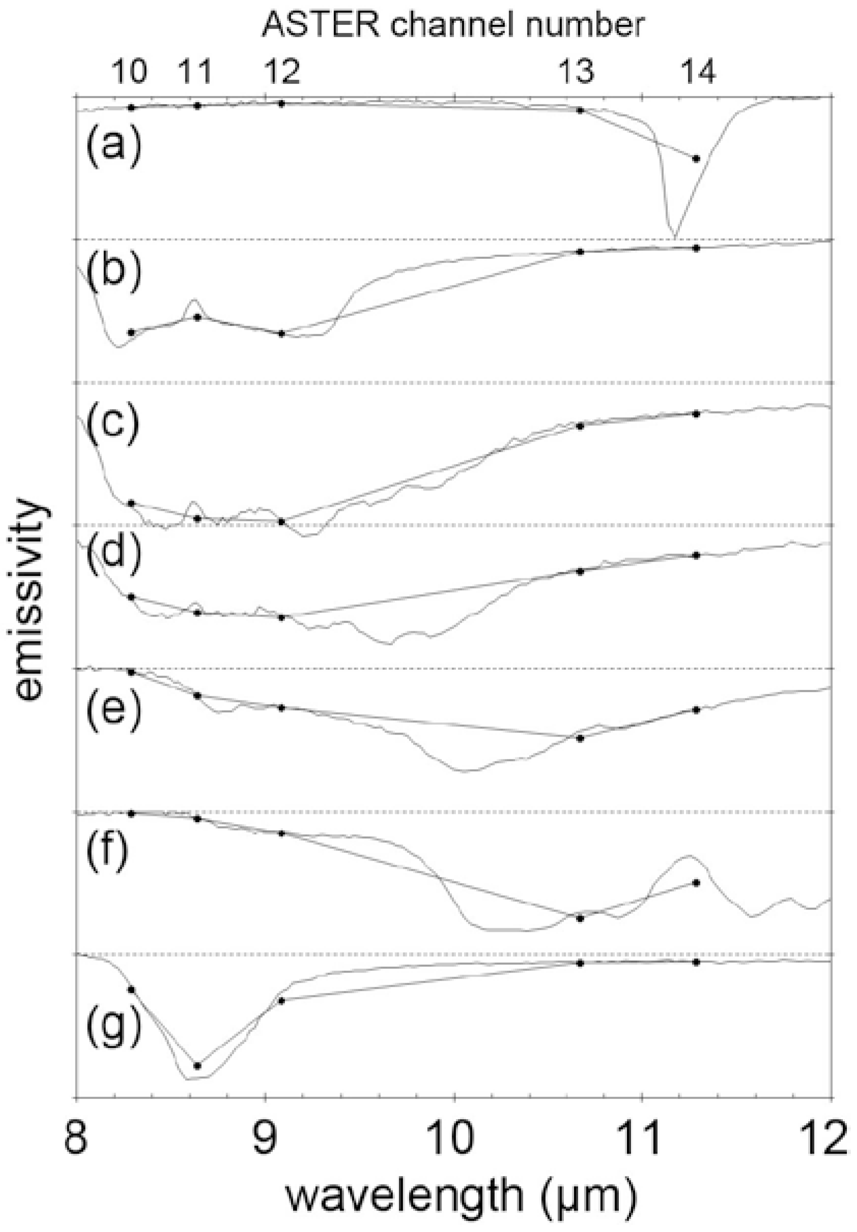
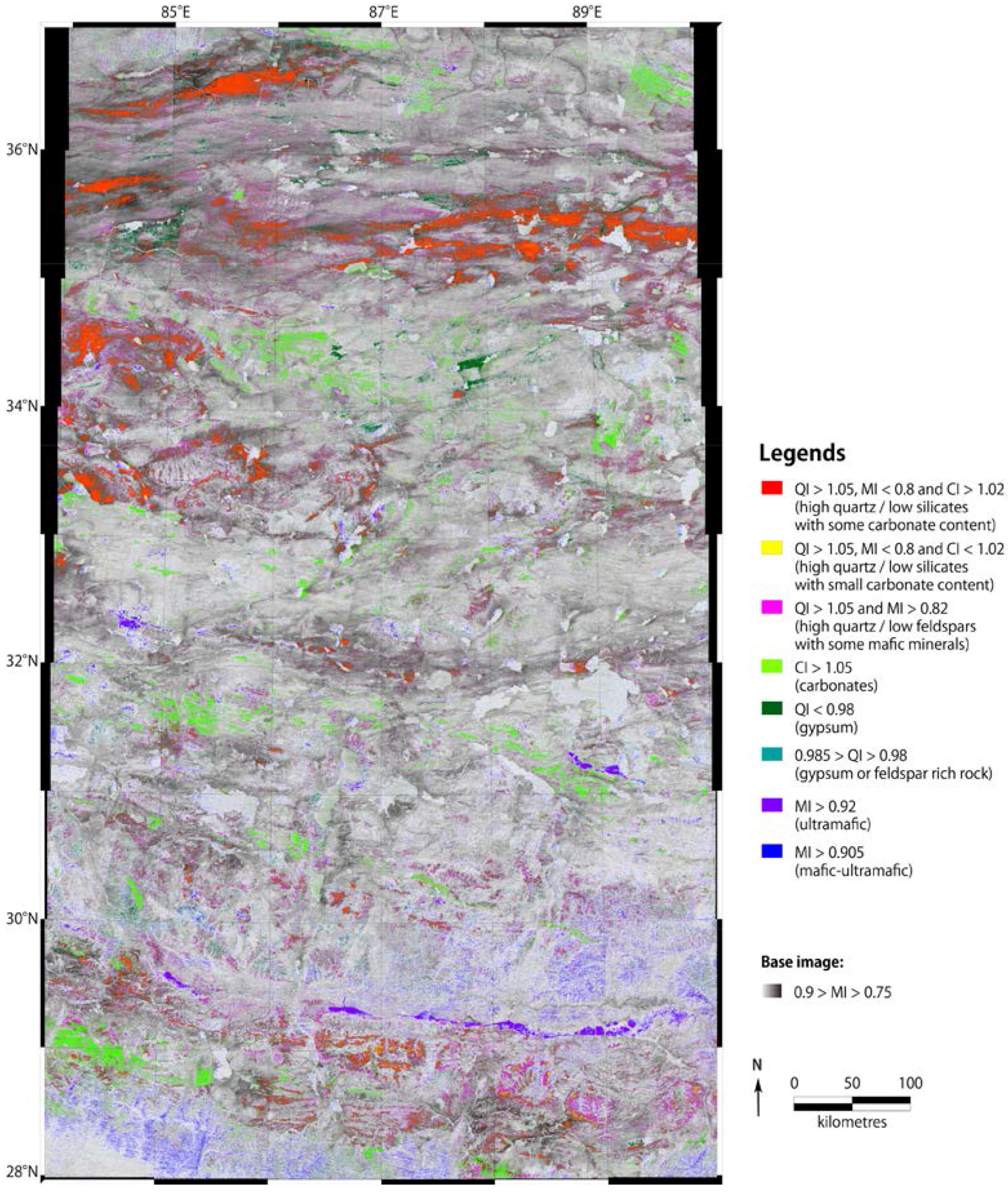
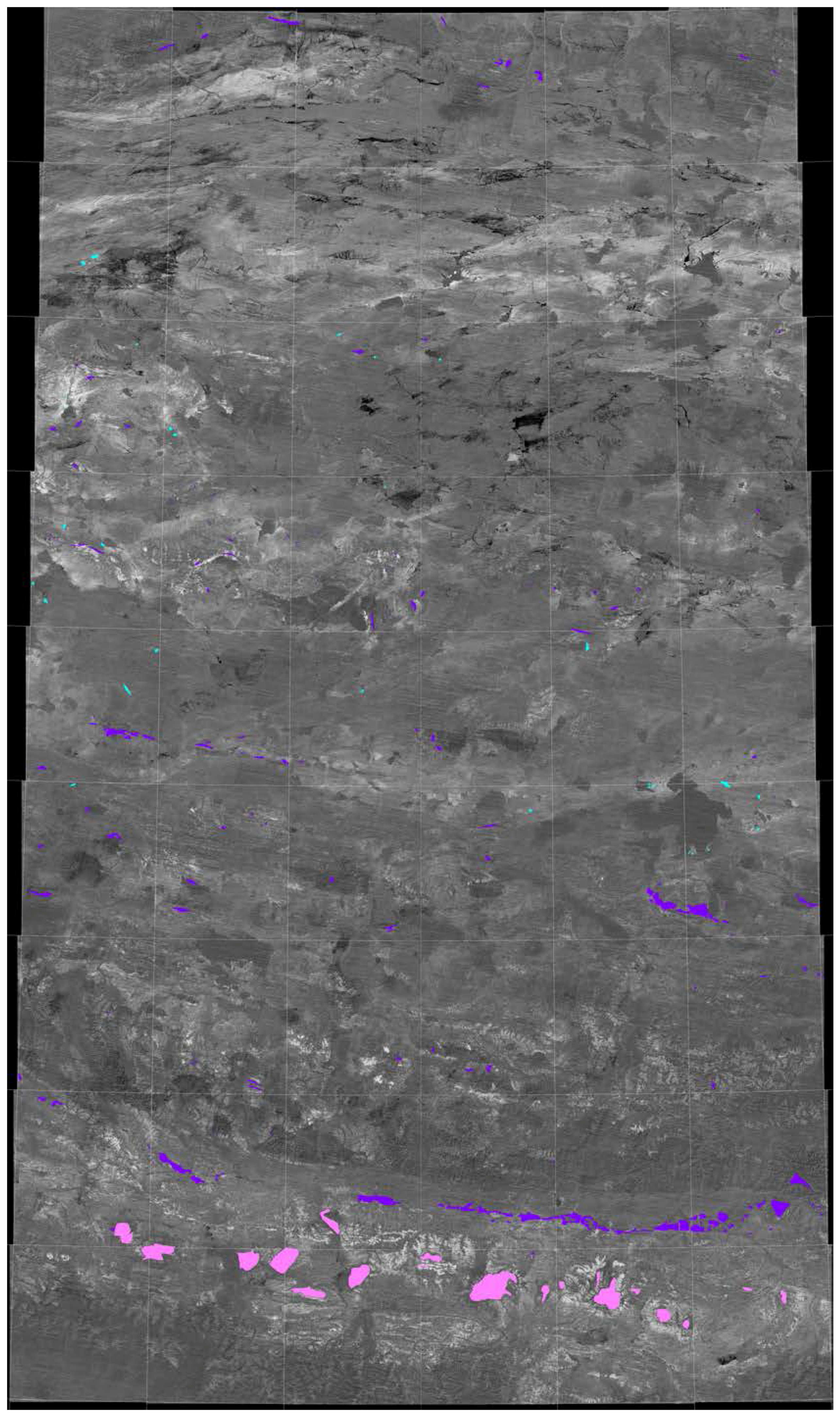
Figure 1. Simplified tectonic map of Tibet and surrounding region, showing the main suture zones in Tibet (modified from References [26,27,28]. Blocks and terranes: ALT-EKL-QL: Altyn Tagh–East Kunlun–Qilian terrane; BS: Baoshan terrane; HM: Himalayan terrane; IC: Indo-China block; KA: Kohistan Arc terrane; LA: Ladakh arc terrane; LC: Lincang–Sukhothai–Chanthaburi Arc terrane; LST: Lhasa terrane; NCB: North China Block; NQT: North Qiangtang terrane; QT: Qiangtang terrane; SP: South Pamir terrane; SPGZ: Songpan-Ganze terrane; SQT: South Qiangtang terrane; TC: Tengchong terrane; TSH: Tianshuihai terrane; WB: West Burma terrane; WKL: West Kunlun terrane. Suture zones: BNS: Bangong-Nujiang Suture; EKLS: East Kunlun Suture; ITS: Indus-Tsangbo Suture; JSS: Jinsha Suture; LSS: Longmu Tso–Shuanghu–Menglian–Inthanon Suture; WKLS: West Kunlun Suture. Basins: QB: Qaidam Basin; KB: Kumkol Basin. Faults: ALT: Altyn Tagh Thrust; ALTF: Altyn Tagh Fault; KKF: Karakorum Fault; LMST: Longmen Shan Thrust; MFT: Main Frontal Thrust; NQLT: North Qilian Thrust; RRF: Red River Fault; SGF: Sagaing Fault; XXF: Xianshui River–Xiaojiang Fault. The dashed red rectangle represents the study area.
Geosciences 06 00039 g001
Figure 2. Mosaic VNIR false color image generated with the ASTER data used in this study, assigned as blue for band 1, green for band 2 and red for band 3 covering the study area bounded by latitude 28° N to 37° N and longitude 84° E to 90° E, using a Universal Transverse Mercator (UTM) map projection. Geographical locations of some cities, mountains, etc., are shown. The yellow rectangle represents the area of Figure 7.
Geosciences 06 00039 g002
Figure 3. Emissivity spectra for common rock types (a) carbonate rock; (b) quartzose sedimentary rock; (c) felsic rock (granite); (d) intermediate rock (diorite); (e) mafic rock (gabbro); (f) ultramafic rock (dunite); (g) gypsum (modified after Ninomiya et al. [17]). Each tick in the Y axis denotes 1.0/0.75 of emissivity except for (b) where it denotes 1.0/0.5 of emissivity.
Geosciences 06 00039 g003
Figure 4. Mosaic color composite image of QI, CI and MI with a linear contrast stretch of 0.97–1.055 (QI; Red), 1.005–1.055 (CI; Green) and 0.79–0.95 (MI; Blue), with ASTER Level-3A products. The areas bounded by the blue polygons were mapped with Level-1B products when Level-3A products were not available. The annotations indicate the locations discussed in the text. The extent of the study area and the map projection are described in the caption in Figure 2.
Geosciences 06 00039 g004
Figure 5. Grayscale image of the indices (a) QI with a linear contrast stretch of the histogram region 0.95 to 1.1; (b) CI with a linear contrast stretch of the histogram region 1.005 to 1.055; and (c) MI with a linear contrast stretch of the histogram region 0.75 to 0.98, produced using the same ASTER dataset of Figure 4 covering the study area. The extent of the study area and the map projection are described in the caption in Figure 2.
Geosciences 06 00039 g005
Figure 6. Detected possible rock types colored for each pixel with the given conditions (see legend) on the indices mapped on the grayscale image of MI (0.75–0.9).
Geosciences 06 00039 g006
Figure 7. Mosaic color composite image of QI, CI and MI covering the region bounded by the latitude 28° N to 29° N and the longitude 86° E to 87° E with (a) ASTER Level-1B products; (b) ASTER Level-2B04 products and (c) ASTER LEVEL-3A products. The coverage in the study area is indicated as a yellow rectangle in Figure 2. A linear contrast stretching of 0.97–1.055 (QI; Red), 1.005–1.055 (CI; Green) and 0.79–0.95 (MI; Blue) is applied on (a,c), and 0.975–1.085 (QI; Red), 1.09–1.145 (CI; Green) and 0.76–0.96 (MI; Blue) is applied on (b). The sub-areas “A” and “B” are enlarged for pointing out the parallax effects. For “A”, the rock unit shown in (c) indicated with an arrow is observed as double in (a,b) as indicated with two arrows. For “B”, the lithological boundary shown across the yellow line in (c) is overlapped and a part of the area is missed along the boundary in (a,b) as indicated with the yellow arrows on the line. These suggest the geometrical mis-registration by the parallax effect occurred for Level-1B and Level-2B products, which are corrected for the Level-3A product. The location of Mt. Cho Oyu is indicated in (c).
Geosciences 06 00039 g007
Figure 8. Distribution map for high-MI mafic-ultramafic rock bodies, high-MI lacustrine deposits and metamorphic domes cored with granite, interpreted with the mosaic images of the indices (Figure 4 and Figure 5), VNIR (Figure 2) and the thematic map with the indices (Figure 6) superimposed on the grayscale image of QI. The red rectangles represent the coverage of Figure 9 and Figure 10, respectively. The information of the previous articles with local geological investigations is embedded as the arrowed lines and texts.
Geosciences 06 00039 g008
Figure 9. Comparison of (a) the Yongzhu-Guomangco ophiolite map (the polygons colored purple; enlarged from Figure 8) and the map of the granitic intrusive bodies (the polygons colored reddish purple) derived in this study using ASTER TIR data superimposed on the color composite image of the indices (Figure 4) with (b) the published geological map based on the field investigations (e.g., [39,40]). The coverage of this figure is shown as the red rectangle in Figure 8.
Geosciences 06 00039 g009
Figure 10. (a) Lithological mapping with the mosaic color composite image of QI, CI and MI around the Malashan domes. The coverage of this image is indicated in Figure 8. The interpreted rock types with this image are A: Quartzose sedimentary layers related to the Tethys, colored yellowish-red; B: Low-grade metamorphic quartzose Tethyan sediments related to the intrusion, colored pure red; C: High-grade metamorphic quartzose Tethyan sediments around metamorphic domes, colored pinkish-red; D: Relatively feldspar-poor granitic rocks related to the domes, colored dark pinkish-purple; E: Feldspar-rich granitic rocks around the domes, colored dark bluish-green; F: Carbonate layers related to the Tethys, colored light green; G: Sulfate deposits, colored deep green; H: Feldspar-rich granitic rocks at the glacier valleys in the north slope of the Himalaya Mountains; (b) Geological map around the western Malashan metamorphic dome area investigated by Aoya et al. [37] embedded in the color composite image of the indices.
Geosciences 06 00039 g010
Table 1. Characteristics of the indices for geological and other materials.
Expected MaterialTypical Geology in the Study AreaFeatures in Indices (Figure 5)Color in Index Image (Figure 4)Detectability with VNIR (Figure 2)Generality
Quartz rich/Feldspars poorQuartzose sedimentary rocksQI > 1.05Pure to yellowish redNot clearConfirmed [14,15,16,17,18,19,21,22,23,26,29,30]
Quartz rich/Silicates poor with some carbonatesQuartzose sedimentary layers related to TethysQI > 1.05, MI < 0.8 and CI > 1.02Yellowish redNot clearNot yet (this study is the first attempt)
Quartz rich/Silicates poor with minor carbonatesLow-grade metamorphic sediments around intrusionsQI > 1.05, M < 0.8 and CI < 1.02Pure redNot clearNot yet (this study is the first attempt)
Quartz rich/Feldspars poor with some mafic mineralsHigher-grade metamorphic sediments around intrusionsQI > 1.05 and MI > 0.82Red to purplish redNot clearNot yet (this study is the first attempt)
CarbonatesMarine sedimentary layers related to TethysCI > 1.05light greenNot clearConfirmed [14,15,16,17,18,19,21,24,25]
SulfatesEvaporates related to neo-TethysQI < 0.98Deep greenNot clearConfirmed [15,16,17,30]
UltramaficOphiolites related to suturesMI > 0.92Light purpleNot clearConfirmed [14,15,16,17,18,25,26,27,28,29,30]
Feldspar-rich granitic rocksGranitic rocks related to island arc (e.g., Gandise batholith)Relatively low QI/Image patternDark bluish greenNot clearPartially confirmed [15,17,19,30]
Feldspar-poor granitic rocksGranitic rocks related to metamorphic domesImage patternDark pinkish purpleNot clearNot yet (this study partially attempts)
Mafic rocksBasalt and gabbroRelatively high MI (≈0.90)Deep blueNot clearPartially confirmed [15,17]
Atmospheric water-High CILight greenPartially (for clouds)-
Snow and ice-Relatively high for all the indicesWhitish greenYes-
Vegetation-Relatively high MI (≈0.89)Greenish blueYes-
Lake water-Relatively high MI (≈0.89), Various values in CIVarious blue to light green colorsYes-

