Where, What, When, and Why Is Bottom Mapping Needed? An On-Line Application to Set Priorities Using Expert Opinion


NOS/NCCOS/MSE/Biogeography Branch, Silver Spring, MD 20910, USA
*
Author to whom correspondence should be addressed.
Geosciences 2018, 8(10), 379; https://doi.org/10.3390/geosciences8100379
Submission received: 18 September 2018
/
Revised: 9 October 2018
/
Accepted: 11 October 2018
/
Published: 16 October 2018
(This article belongs to the Special Issue Geological Seafloor Mapping)
Abstract
:Globally, there is a lack of resources to survey the vast seafloor areas in need of basic mapping data. Consequently, smaller areas must be prioritized to address the most urgent needs. We developed a systematic, quantitative approach and on-line application to gather mapping suggestions from diverse stakeholders. Participants are each provided with 100 virtual coins to place throughout a region of interest to convey their mapping priorities. Inputs are standardized into a spatial framework using a grid and pull-down menus. These enabled participants to convey the types of mapping products that they need, the rationale used to justify their needs, and the locations that they prioritize for mapping. This system was implemented in a proposed National Marine Sanctuary encompassing 2784 km2 of Lake Michigan, Wisconsin. We demonstrate key analyses of the outputs, including coin counts, cell ranking, and multivariate cluster analysis for isolating high priority topics and locations. These techniques partition the priorities among the disciplines of the respondents, their selected justifications, and types of desired map products. The results enable respondents to identify potential collaborations to achieve common goals and more effectively invest limited mapping funds. The approach can be scaled to accommodate larger geographic areas and numbers of participants and is not limited to seafloor mapping.
1. Introduction
Over 150 of the Earth’s nearly 200 countries have coastal and marine areas as part of their exclusive economic zone (EEZ). Over half of these coastal countries possess more area under the surface of the sea than above it (marineregions.org, accessed 6 June 2018). Mapping the seafloor of these areas is an essential task for exploring, using, and managing the resources of these vast undersea regions [1]. Despite the need to understand basic information about the seafloor, most countries lack the resources to map their entire EEZ. For example, the United States, which has the second largest EEZ in the world (11.3 million km2) and among the greatest financial and technological capabilities to map it, has only surveyed 41% of its seafloor [2]. Moreover, much of that “mapped” area has fewer than 3 soundings per hectare, and was mapped with obsolete technologies, such as lead lines. Worldwide, the situation is more dire. Less than 9% of the seafloor has been mapped using modern technologies, such as multibeam sonar; filling the survey gaps would require a conservative estimate of ~1000 years [1]. Given the enormous area of seafloor that needs to be mapped and the limited resources available for mapping, it has become clear that smaller areas should be prioritized for initial mapping and that multiple groups could combine resources to increase mapping efficiency of many areas if they were better informed about locations with overlapping interest.
To meet this need, several approaches have recently been devised to assist groups of people with the task of prioritizing and coordinating seafloor mapping at a regional scale. Most use a standardized, grid-based framework to partition the area of interest, and seek to understand the rationale behind priority choices. For example, the State of California convened a workshop to gather mapping suggestions from multiple organizations, using the California Division of Fish and Game commercial fishing blocks as a spatial framework [3]. Participants were each provided 10 votes that they were instructed to place within the blocks which they deemed the highest priority for mapping. Sticky dots, poster-sized charts, and maps were used to gather input on where mapping was needed and the justification for each selection. More recent prioritization processes have gathered input using a participatory geographic information system (pGIS) accessed on-line [4,5]. Participants in New York’s Long Island Sound and the State of Washington used grid-based frameworks to assign priority levels of high, medium, or low using point-and-click selection tools to choose and attribute grid cells. Priority levels and a list of possible justifications were assigned using pull-down menus that were pre-populated with choices established by regional advisory teams. Other on-line tools lacking a standardized grid-based framework have also been explored for identifying mapping gaps or priorities, such as SeaSketch (www.seasketch.org), Social Values for Ecosystem Services (SolVES) [6], NOAA’s Bathymetry Gap Analysis GeoPlatform [2], and other tools in ArcGIS (www.esri.com), however, these would require additional modification and were not specifically designed to collect the needed types of input.
In this study, we combined the best aspects of earlier approaches and modified them to enable more quantitative input in setting mapping priorities. The design was guided by the principle that coordination of multiple partners with overlapping priorities can result in collaborative projects and sharing of resources, but only if everyone’s mapping needs are articulated in a structured framework [3,4,5]. The core elements of the approach used here included collecting all information using an on-line pGIS application, partitioning the area of interest using a uniform grid, using virtual coins placed on the grid as a means of identifying priorities, and assigning attributes using pull-down menus. The approach efficiently and systematically gathered quantitative input from multiple individuals on their mapping priorities. Participants could convey where to map, what types of map products are needed, when the products are needed, and a justification of why their suggested locations are a priority for mapping. The system standardized inputs into a GIS framework that enabled us to identify groups of individuals with shared interests and collaborative opportunities.
This new application for understanding mapping priorities was used in the State of Wisconsin to assist with planning for the proposed Wisconsin–Lake Michigan National Marine Sanctuary [7,8]. The planning area focused on a 2784 km2 portion of lakebed between the cities of Kewaunee and Port Washington, Wisconsin. The area includes dozens of known and suspected shipwrecks [9], ecologically significant habitats [10], and geological formations [11,12], although the details and dynamics of these lakebed features remain largely unmapped by modern standards. Existing mapping data are coarse, dated, and typically provide only depth information. For nearly 90% of the area, mapping data consist of single-beam hydrographic surveys collected before 1950 at a spacing of 1–2 km between soundings [8].
Like most areas in the world, the lack of recent maps of the lakebed is due to several factors. The study area encompasses a large area by itself, but must also compete with the rest of the Great Lakes for mapping resources. Only 4% of the entire US Great Lakes has been mapped, with a density of at least 1 sounding per hectare [2]. The study area is also deep (av 65 m, max 138 m), and much of the lakebed lies below the penetrative capability of airborne- and satellite-based sensors that can efficiently cover broad areas (e.g., LiDAR). This means that mapping must be done from the limited number of survey boats or autonomous underwater vehicles (AUV) in the Great Lakes, and using sensors such as side-scan, interferometric or multibeam sonar, magnetometers, or camera systems depending on the desired map products. As a result of these constraints and limited funding, it is recognized that the entire area cannot be mapped in a short timeframe, and that smaller areas should be prioritized to address the most urgent needs [13].
Our objectives with this study were to (1) demonstrate the processes that we used to gather suggestions for lakebed mapping, so that others may implement similar techniques elsewhere, and (2) provide examples of some of the most essential analyses that can be performed with the data. These analyses include an accounting of which justifications and map products are most common, which occur together at the same locations, where highest priorities are for different interest groups, and where highest priorities are overall.
2. Materials and Methods
2.1. Web-Based Prioritization Application
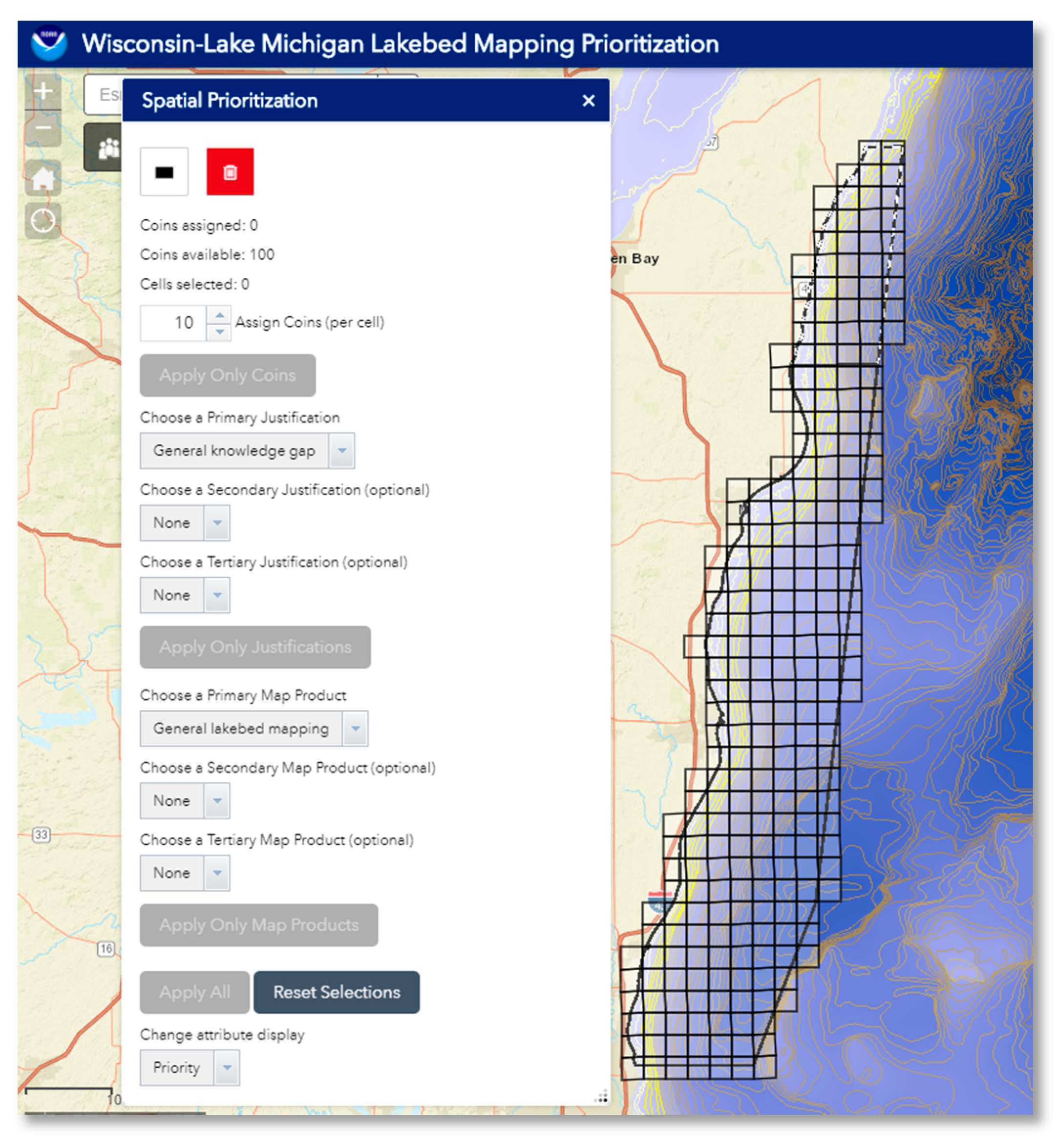
The application was designed using ESRI’s Web AppBuilder, vesion 2.8 (ESRI, Redlands, CA, USA) framework with best-practices of pGIS as a guide [14]. Participants logged into the on-line application and used a customized suite of selection tools and pull-down menus to easily convey their mapping priorities (Figure 1). Customization of the application was guided by convening a Technical Advisory Team (TAT) that consisted of local experts who have an interest or expertise in lakebed mapping. The TAT reviewed the application, recommended locally relevant datasets and options for users to select in the menus, and helped identify suitable respondents to participate [8].
Respondents were chosen to span a diversity of fields (i.e., ecology, limnology, fisheries, geology, history, and coastal management) and were from federal, state, county, university, and other groups (Table S1). The common characteristic among all participants was that they relied heavily on bottom maps within the study area as a key input to their research or management decisions. It should be noted that choice of respondents is vitally important to obtain useful results since the outcome of the prioritization process is dependent upon their participation. Each respondent was provided a link to the application and a unique login ID. Respondents could access the application at their convenience from any computer with an internet connection. Respondents were trained how to use the application during in-person meetings or webinars conducted in November 2017. During the training, respondents were provided background on the objectives of the project, shown how to access the menus in the system, and stepped-through some example scenarios during a demonstration of the application. Once trained, the respondents were given a deadline of several weeks to enter their suggestions for mapping.
The application was comprised of two main components, a data viewer, and a prioritization interface. The data viewer included spatial layers depicting the extent, date of acquisition, and resolution of available lakebed surveys and related mapping products. Respondents could view and query this information to understand the limitations of existing information, gaps in existing maps, and help identify priority areas for future mapping. The data viewer can include any other spatial data that can inform mapping decisions. The other part of the application, the prioritization interface, consisted of the grid-based framework wherein respondents could input their mapping priorities.
Each respondent was given 100 virtual coins to place anywhere within the study area that they felt was a priority for future mapping. Respondents were told to allocate and prioritize the placement of their coins as they would allocate their limited mapping resources over the next several years. The project area was divided into 4 × 4 km grid cells to standardize the size of the area designated during coin placement (Figure 1). This grid consisted of 261 equal-area cells aligned to the US National Grid/Universal Transverse Mercator coordinate system. Respondents could place from 1 to a maximum of 10 coins in any cell that they wished to prioritize for future mapping. This constraint forced respondents to allocate their limited coins into a minimum of 10 cells (10 coins per cell) to a maximum of 100 cells (1 coin per cell), or 4% to 38% of the study area depending on the number of coins allocated per cell.
Respondents were instructed to not only allocate coins to convey where mapping is needed, but also when mapping products are needed. More coins denoted greater urgency based on the following general guidance: 8–10 coins indicates a high priority or needed immediately, 4–7 coins means maps are needed in the next 2 to 4 years, and only 1–3 coins indicates a longer term priority needed in 5 to 10 years. In the application, respondents first selected the cell (or cells) they wish to prioritize using click and drag menu options. A pull-down menu allowed respondents to select the number of coins (up to 10) they want to place in that cell(s). As coins were assigned, the system tracked and displayed the number of coins remaining to be allocated.
After assigning coins, respondents then conveyed what types of Map Products are needed in each selected cell. Simple pull-down menus were prepopulated with several types of map products to choose from (Table 1) based on input from the TAT along with the default setting of “General lakebed mapping”. Respondents were required to indicate a primary Map Product desired at each location and could optionally designate a secondary and tertiary Map Product. Last, respondents indicated why they chose each cell, again using pull-down menus prepopulated with a list of locally relevant Justifications (Table 2), along with the default setting of “General knowledge gap”. Respondents were required to select a primary Justification, but could also optionally select a secondary and tertiary rationale as well. The application saved each input as it was made on-line, and respondents could return to the system to edit their selections, in any order, as many times as they wished until the submission deadline.
2.2. Data Analysis
2.2.1. Data Compilation
A total of 22 respondents entered mapping suggestions into the on-line prioritization application. The 261 grid cells and corresponding priorities from the 22 respondents were compiled into a single table consisting of 5742 rows. Each row, therefore, consisted of a single respondent’s priorities for a given cell with columns noting the number of coins assigned, Justifications (up to three), and Map Products (up to three). The general areas of expertise for each respondent were also linked to this table (i.e., ecology, geology, history, or other) which served as the basis for all subsequent analyses. Key example analyses of this dataset are described, however, this suite of methods is not comprehensive, and should be modified to address needs specific to other projects.
2.2.2. Determining Which Justifications and Map Products Are Most Commonly Selected
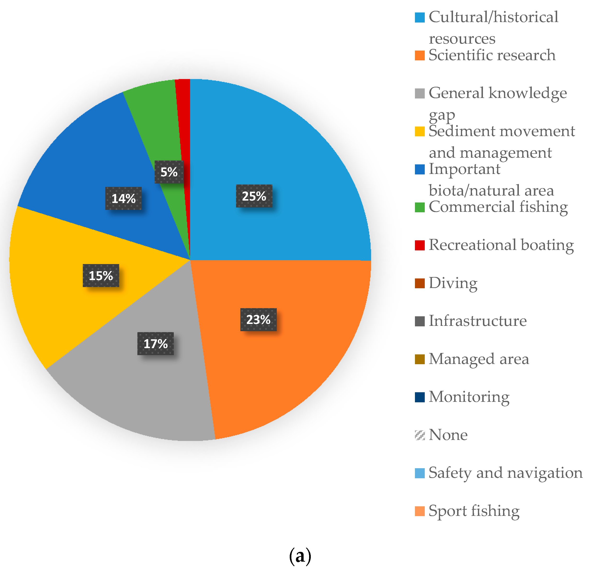
Simple figures, such as pie or bar graphs, provide effective means to convey which Justifications and Map Products are most commonly selected by respondents. As examples for this study, the total number of coins associated with primary, secondary, and tertiary Justifications were tallied separately, and their relative proportions were visualized using pie charts. Similarly, the total number of coins associated with primary, secondary, and tertiary Map Products were tallied and used to produce pie charts. Note that responses could also be pooled across all priority levels if that were of interest.
2.2.3. Determining Which Justifications and Map Products Are Commonly Listed Together
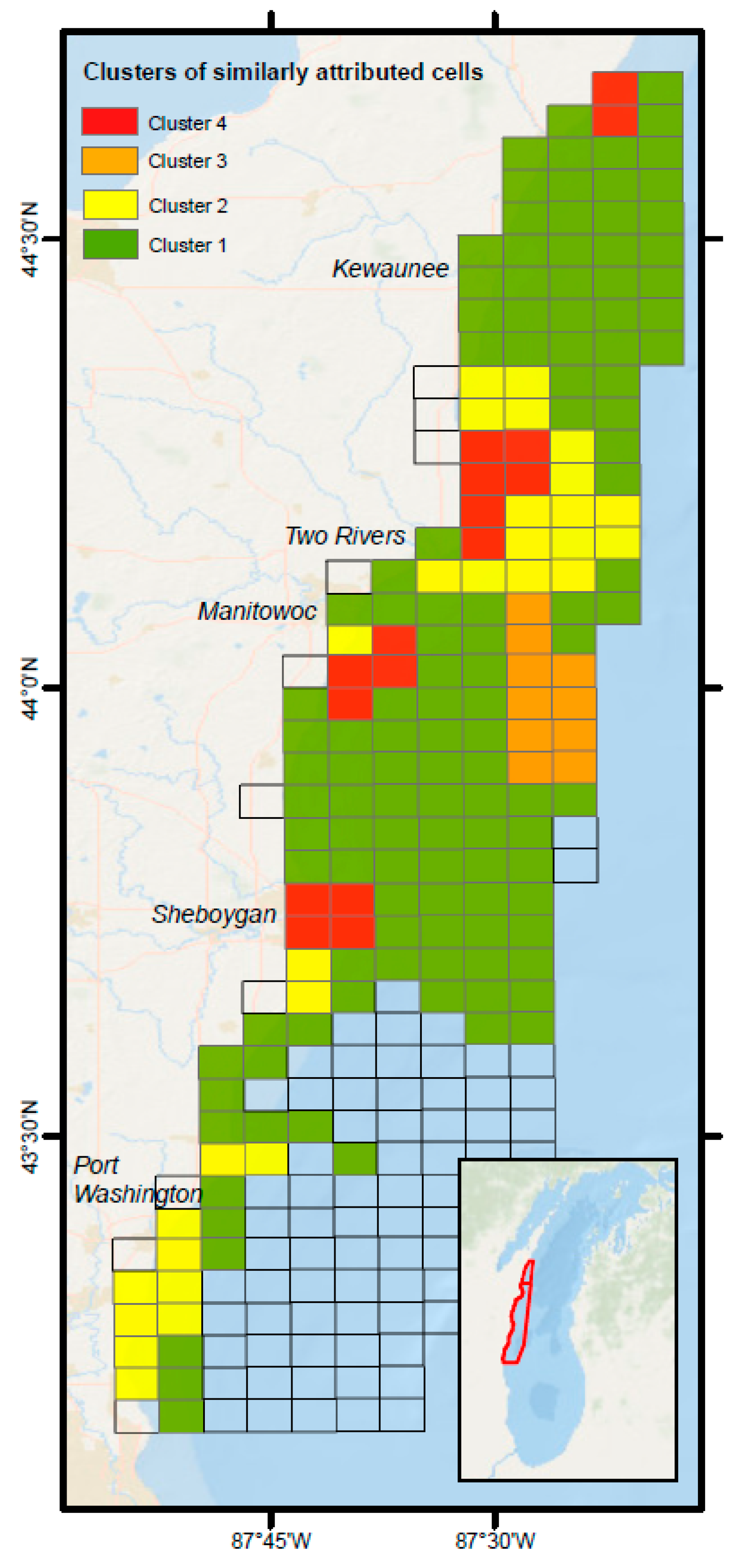
Hierarchical cluster analysis was used to explore if particular combinations of Justifications and/or Map Products commonly occurred together. For this analysis, a table was created with all 261 grid cells as rows and the total number of coins within each category of Justification and Map Product (any priority level) selected by respondents as columns. Grid cells with no coins were excluded. Remaining grid cells were then subjected to several clustering algorithms using standardized and unstandardized data transformations, in order to identify the consistent patterns of clustering regardless of algorithm or standardization used. Cells were clustered based on the number of coins under each Justification and Map Product. The number of clusters was set to where dissimilarity among clusters was large, and multiple algorithms showed similar results. Within each cluster, the average number of coins in each Justification and/or Map Product category were calculated to understand the important variables responsible for cluster membership. We also plotted cluster membership back onto the prioritization grid to examine the spatial patterns of cluster distribution.
Note that, in this example, the respondents’ choices for each grid cell were pooled, meaning that co-occurring Justifications and Map Products were not necessarily selected by the same respondent in a given cell. This analysis could also be performed at the individual respondent level, if it is desired to explicitly link the Justifications and Map Products of each respondent. The individual results can then be summarized to investigate overall patterns.
2.2.4. Where Are the Cells of Highest Priority for Future Mapping?
Coin tallies and other values within the grid of 261 cells can be summarized and plotted to identify hotspots of relatively high priority for future mapping. As examples for this study, data were summarized to examine how the respondents allocated coins overall, within various fields of expertise, and within the most commonly used Justifications and Map Products identified in Section 2.2.2 First, we partitioned the responses into a variety of subsets to understand which variables could be influential on the overall patterns of high priority. We plotted the total number of coins per cell, based on the type of general expertise of the respondents (i.e., ecological, geological, or historical). Following that, we partitioned responses into the total number of coins per cell within each of the top 5 Justifications identified in Section 2.2.2 Preliminary analysis revealed these to be “Cultural/historical resources”, “Scientific research”, “General knowledge gap”, “Sediment movement and management”, and “Important biota/natural area”. We also partitioned the responses into the total number of coins per cell within each of the top 2 Map Products, as identified in Section 2.2.2 Preliminary analysis revealed these to be “General lakebed mapping” and “Bathymetry/digital elevation model”.
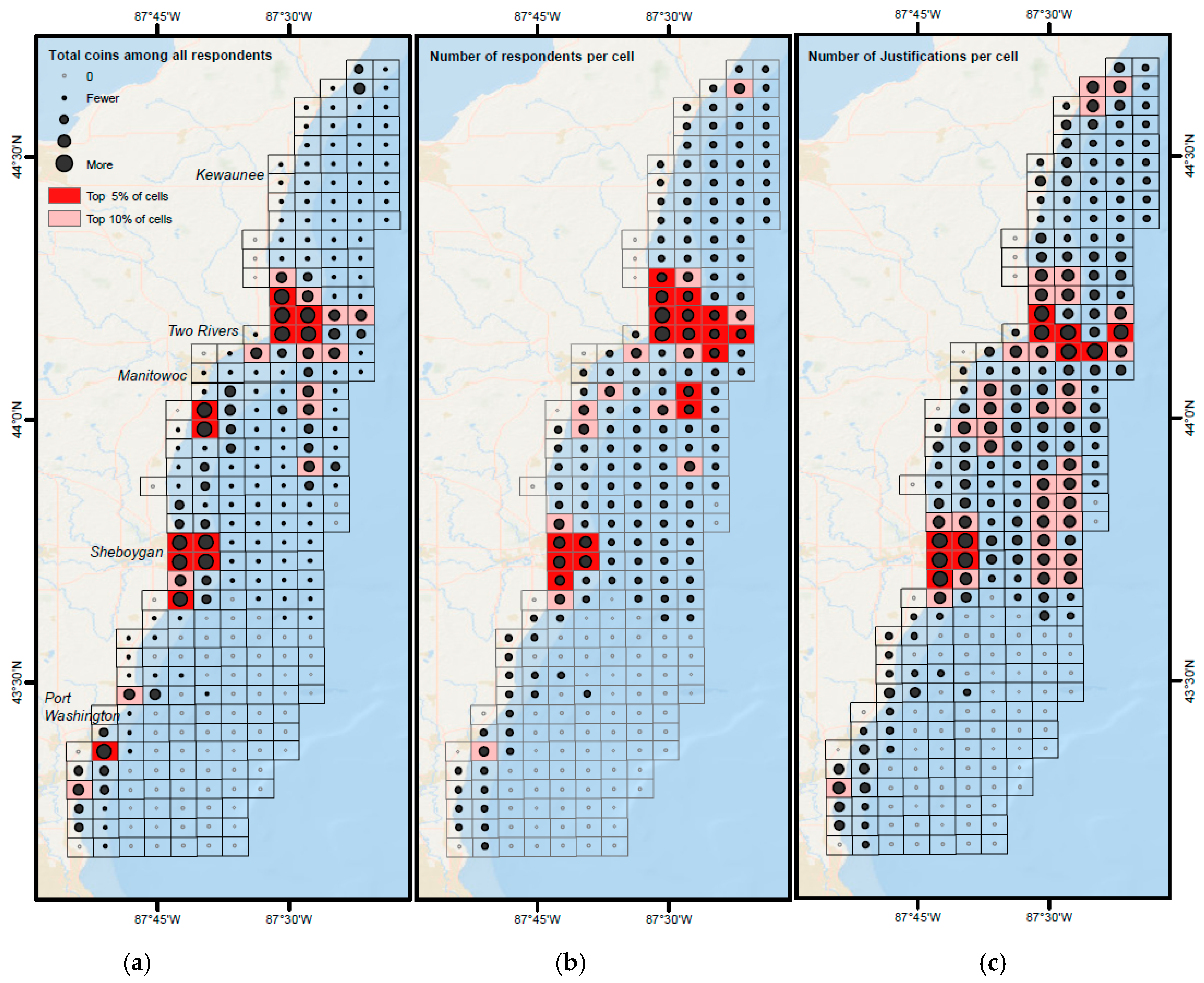
Next, more general indicators of mapping priorities, incorporating all the responses, were computed. For this, we calculated the simple sum of all the coins by all respondents in each grid cell, the number of respondents assigning at least one coin in each grid cell, and the number of different Justifications that occurred in each cell. These summary maps represent measures of overall importance across all respondents.
Cells representing the highest priorities for future mapping were identified from each of these different summary maps. Cell values (e.g., total number of coins) in each summary map were ranked from highest to lowest, and the top 10 percent of highest value cells (26 cells in each map plus any ties for the 26th value) were marked and labelled as “high priority” cells. We also marked the top 5 percent of cells as “highest priority” cells. We then compared these maps for overlap in high priority cells.
It was also useful to look at some variables in composite. For this part of the analysis, we wanted to identify the highest priority cells of the greatest importance to the broadest diversity of respondents. We began by using the three most general summary values, as described above, including the sum of all coins in a cell, the number of respondents in a cell, and the number of different Justifications in a cell. We ranked the cells from smallest to largest values, based on these three variables as described previously, converted the rankings to percentiles to standardize them (since there were unequal numbers of ties and raw ranks covered different scales) and, then, added the percentiles together and plotted the results on a continuous scale. This holistic measure of importance yielded a composite value of the highest combined number of coins, number of respondents, and number of Justifications.
3. Results
A total of 22 respondents entered suggestions into the on-line prioritization tool, and allocated a combined total of 2200 coins into the grid cells to denote their suggestions for future lakebed mapping. It is unknown how many respondents, and to what extent, may have used the data viewer or independent datasets to assist with their selections. In the future, this important information could be gathered using check boxes, with options such as “1. I am familiar with available mapping data for this region, 2. I used the data viewer, 3. I used other information to guide my selections”.
3.1. Which Justifications and Map Products Were Most Common?
The proportion of coins that were assigned using the Justification categories at the primary, secondary, and tertiary levels revealed that there were 5 main Justifications most frequently selected (Figure 2a). The topics “Cultural/historical resources” and “Scientific research”, together, comprised nearly half of all the primary Justifications chosen. These were followed by “General knowledge gap”, “Sediment movement and management”, and “Important biota/natural area”, which each comprised 14–17% of primary Justifications. The eight remaining choices were seldom used, and each accounted for less than 5% of the assigned coins. Patterns were similar for secondary and tertiary Justifications. These 5 most dominant categories were used in the subsequent analysis to identify high priority areas.
The proportion of coins that were assigned using the Map Product categories at the primary, secondary, and tertiary levels revealed 2 main desired products (Figure 2b). The products “General lakebed mapping” and “Bathymetry/digital elevation model” were, by far, associated with the greatest number of coins and, together, comprised ~75% of all primary Map Product types selected. Secondary and tertiary Map Products most commonly selected were “Lakebed surface type”, “Sub-bottom geology”, and “Ground-truth data”. The 2 most dominant Primary categories for Map Product were used in the subsequent analysis to identify high priority areas.
3.2. Were Particular Justifications and Map Products Commonly Listed together?
Cluster analysis based on the number of coins associated with the various Justifications and Map Products revealed 4 groups of cells that had a similar suite of attributes (Table 3). Cluster 1 included the largest number of cells. It was comprised of cells with low coin totals and, therefore, likely represented lower priorities overall. Cells in Cluster 2 had moderately high coin totals for “Scientific research” and “Sediment movement and management” as Justifications, and “Bathymetry/digital elevation model” and “Sub-bottom geology” as desired Map Products. This combination of choices suggests that this group of cells may only be of interest to geological or sediment management studies. Cluster 3 was the smallest group, and had high coin totals for “Cultural/historical resources” and “Scientific research” as Justifications, almost exclusively. These cells also typically had high coin totals for “Lakebed surface type” and “Sub-bottom geology”, and differed from the other clusters in being the only group with high coin totals in the “Ferrous object detections/magnetic anomalies” category. This combination of choices suggests that this group of cells were of particular interest to shipwreck/cultural studies. Lastly, Cluster 4 was comprised of cells with high coin totals in several categories, suggesting high overlap in interest spread among diverse justifications. Justifications occurring together in this cluster were “Cultural/historical resources”, “Important biota/natural area”, and “Scientific research”. Map Products requested together in this cluster were “Bathymetry/digital elevation model”, “Lakebed surface type”, and “Sub-bottom geology”. This was the only cluster with even a moderate number of coins Justified based on “Fishing”, and the only cluster with a large number of coins under the “Ground-truth data” category of Map Products.
Plotting these clusters revealed several notable patterns (Figure 3). Cells with no coins assigned by any respondent and therefore eliminated from the cluster analysis, were grouped offshore of Port Washington in the southern 1/3 of the study area. Cells in Cluster 1, representative of only modest interest among respondents, occurred as two large groups off the City of Kewaunee, and between Manitowoc and Sheboygan. Cluster 2, potentially representative of cells of interest only to geologists, were mostly located offshore of Two Rivers and along the coast south of Port Washington. Cluster 3, apparently of interest only to historians, was located in a longitudinal strip well offshore of Manitowoc. Cluster 4, which had the highest coins totals in the greatest diversity of categories, occurred in four regions. These were nearshore off Sheboygan, Manitowoc, Two Rivers, and at the northern edge of the study area.
3.3. Where Are the Cells of Highest Priority for Future Mapping?
Locations of highest priority for future mapping differed, depending on whether the input of the respondents was partitioned by expertise, Justification, Map Products, or was considered holistically. When the coin allocations were partitioned based on the primary topic of expertise of the respondents, key differences in priority areas became apparent (Figure 4a–c). Respondents in the geologist group (n = 4) allocated their coins in only two areas, eastward from the promontory off Two Rivers and nearshore south of Port Washington (Figure 4a). In contrast, respondents in the historian group (n = 5) allocated most of their coins in the space between the top areas selected by the geologists. Historians prioritized a large group of cells extending offshore south of Manitowoc, and three groups of cells north, south, and offshore from Sheboygan, as well as a strip of cells extending offshore north of Port Washington (Figure 4b). The ecologists (n = 9) were somewhat more diffuse in their allocations, as might be expected, with a greater number of individuals placing coins. Four areas comprised the top 5th percentile by ecologists, two cells at the northern extremity of the study area, a group of nearshore cells east of Two Rivers, and also nearshore cells south of Manitowoc and off Sheboygan (Figure 4c).
When we partitioned the responses based on the Justifications that were selected in each cell, additional patterns became apparent (Figure S1a–e). Examining the top 5 Justifications separately revealed some additional patterns of interest. The more broadly applicable Justifications of “General knowledge gap” and “Scientific research” were somewhat diffuse in their spatial distribution, but were primarily used in the middle and northern thirds of the study area (Figure S1a–b). Not surprisingly, the “Cultural/historical resources” Justification was used primarily in the middle 1/3 of the study area, and generally corresponded to the area prioritized highly by historians (Figure S1c). The “Sediment movement and management” Justification had the highest values and overlaps with the two areas selected most often by geologists (Figure S1d). There was, however, an additional area near Sheboygan justified with that rationale that was not picked by geologists. Last, the “Important biota/natural area” Justification had a somewhat different pattern (Figure S1e). The largest area in the top 5th percentile with this Justification was south of Manitowoc and extended offshore. Interestingly, this group of cells overlapped the same block of cells that were noted as a high priority by the respondents with historical expertise.
When we partitioned the responses based on the two most commonly selected Map Products, additional patterns became apparent. Most of the coins allocated in the broad Map Product category of “General lakebed mapping” were located in the middle 1/3 of the study area with highest priority cells eastward off Two Rivers, south of Manitowoc, and near Sheboygan (Figure S2a). The Map Product “Bathymetry/digital elevation model” covered a similar pattern only shifted to the north (Figure S2b).
When respondent’s data was considered holistically, cells with the highest total number of coins allocated among all respondents occurred in 4 regions (Figure 5a). The largest concentrations of cells in the top 5th percentile of total coins were northeast of Two Rivers and in the nearshore waters off Sheboygan. Two smaller areas of high-value cells were located in nearshore waters off Port Washington and south of Manitowoc. A somewhat similar pattern was found when considering the number of respondents that allocated coins in each cell (Figure 5b), wherein the same general groups of cells off Two Rivers and Sheboygan had the highest value (top 5th percentile). The number of different Justifications was highest in the middle third of the study area, with two concentrations of especially high diversity, off Sheboygan and eastward from Two Rivers (Figure 5c). This reflects diverse reasons for mapping those areas. Not only do these 3 figures convey areas of high priority, but they also show large parts of the study area where there was little or no interest in lakebed mapping. No coins were assigned by any of the 22 respondents to 84 of the 261 cells in the study area. These were primarily in the southeastern 1/3 of the area offshore of Port Washington.
The cells with the highest combined ranks based on total number of coins, number of respondents, and diversity of Justifications are plotted in Figure 6. Highest values were concentrated in small groups of cells off Sheboygan and eastward from Two Rivers. Moderately high values were more diffuse, with a loose grouping of cells south of Manitowoc and Two Rivers and a couple of isolated cells elsewhere.
4. Discussion
We designed an on-line application to gather experts’ opinions regarding their priorities for bottom mapping. The system allowed respondents to indicate where mapping is needed, the types of map products that are required, the urgency of the need, and a rationale to justify their priorities. We presented several types of analyses that, while not comprehensive, are among the most essential for coordinating and seeking funds for mapping projects in high priority areas. The system was implemented in a proposed protected area along the Wisconsin coast of Lake Michigan [15] although it can be applied to any type of spatial prioritization process. Based on analysis of the responses in the Lake Michigan study area, 3–4 small groups of cells emerged as the highest priority for many experts. These were located east of Two Rivers, off Sheboygan, and south of Manitowoc, and consisted of 3–5 contiguous cells. These cells could be the focus of upcoming mapping initiatives to fulfill the most urgent needs for the greatest number of interest groups [8]. The results of the analysis were presented to the respondents for feedback, and to foster collaborative endeavors among them.
Knowledge of which Justifications and Map Products were most commonly used and co-occurred spatially is important to guide mapping strategies, align goals with appropriate funding sources and, ultimately, to facilitate survey proposals. The information gathered in this process can be cited to funding entities to support mapping initiatives.
Cluster analysis was shown as a useful technique to efficiently partition the area into subsets on a single map based on desired Map Products and Justifications. In the example shown here, Cluster 1 had modest but measurable interest, but could be considered, collectively, as low priority. Clusters 2 and 3 were of interest to specialized groups. Cluster 4 was prioritized by multiple groups for multiple reasons, and could be considered as a high priority among the respondents with the most potential for collaboration. Provided that the clusters are adequately described, this single layer is an effective and efficient way to summarize and convey the results back to respondents and other users. In cases where the suggestions of the respondents do not separate into clearly distinct groups, a technique more suitable for continuous gradations may provide a better approach.
Analysis and maps partitioning of the priorities among different variables, were among the most important in the analysis. Plotting the data in a diversity of ways allowed us to disentangle the various priorities among experts from different fields. This approach not only identifies important areas unique to each group, but perhaps, more importantly, also identifies areas that are a high priority for more than one field of experts. Overlapping interest among many respondents in the same cell(s) may represent some of the best opportunities for collaboration. Some noteworthy examples of collaborative opportunities include the nearshore cells off Sheboygan and the cells extending offshore eastward from Two Rivers. These cells had the highest number of respondents and the greatest diversity of Justifications used during coin allocation. This suggests there are both ample numbers of potential collaborators in this area and, also, multiple rationales for mapping which can attract partners and funding from various sources. In particular, the inshore cells east of Two Rivers were high priorities for ecologists and geologists to map “Important biota/natural area” and “Sediment transport/management”. Respondents often justified these same cells as important to map due to “Cultural/historical resources”. These collaborative opportunities were only made apparent and quantified through this analysis, that brought together professionals with a variety of interests and backgrounds that otherwise would have been unlikely to connect and share their mapping interests.
The prioritization process also revealed that collaboration need not be limited to those interested in the exact same place and mapping product. For example, perhaps two groups need the same map product or survey equipment (e.g., sonar unit), but in different places. The cost and time of renting and/or mobilizing such equipment on survey vessels is not trivial, and could be the basis of cost sharing for back-to-back survey missions, even in different areas. Using the data collected here, respondents can identify other groups with similar equipment needs. There are also collaborative opportunities when the map product and equipment needs differ, but the area of interest is the same. In such cases, more than one type of survey instrument can often be deployed, concurrently, on the same survey vessel to collect multiple data streams for different map products. For example, multibeam, side-scan, and split-beam sonar systems can be deployed, all at once, to map bathymetry, surface types, and fish populations.
It is also useful to recognize that some places were identified as high priority, but only for one particular group or purpose. For example, only the geologists interested in “Sediment transport/management” selected the nearshore cells off Port Washington as a high priority. Similarly, only the historians were particularly interested in the cells in the deepest part of the study area offshore from Sheboygan, and only the ecologists prioritized the northernmost cells of the area. Such differences are important to know, so these groups can recognize that they may have to work independently in these areas. They could either focus their mapping resources at those sites, since it appears less likely that others may be interested, or they may wish to refocus their interest elsewhere, where greater resource sharing and collaborative opportunities may be had.
We designed this process to facilitate outreach among groups that would perhaps not normally collaborate. Once the results have been compiled and summarized for processes such as this, it is essential that others can access and use this information to coordinate their activities. Contact information should be provided among respondents and to others with an interest in mapping the area. Summary grid values should be published and made accessible, while taking into consideration any sensitivities or rights to privacy expressed by individual respondents. Although participation in this process necessarily demonstrates a desire to share one’s opinion, this expectation should be made clear at the outset of the process [14]. Sharing the findings with the growing number of local and regional groups that seek to coordinate mapping will be especially important. In our case, the Great Lakes Bottom Mapping Workgroup [13] and NOAA’s Integrated Ocean and Coastal Mapping program (https://iocm.noaa.gov/) were involved from the outset, and are anticipated to be key users of the results.
A review of the evolution of the prioritization approaches that have been recently conducted [3,4,5] reveals some useful guidance for those interested in conducting similar endeavors elsewhere. First, pGIS is an ideal tool for gathering the needed data, provided that it is properly implemented through representative and unbiased participants who are giving informed consent to the open exchange of information [14]. pGIS offers a structured, visual, accessible platform that standardizes and saves inputs for easy analysis, archiving, and dissemination.
Second, a regular grid is a useful spatial framework for collecting the necessary information. Having the grid cells be the same size standardizes the area and weight of priorities equally across the region of interest. Irregular grids, where cells are larger in deeper waters, for example, may be useful for some purposes but may, ultimately, complicate the comparison of priorities among areas. In addition to the size of cells in the selection framework, the total number of cells should be carefully considered. The number of cells is dependent primarily on the desired resolution of the output and the overall size of the area. A prioritization grid comprised of more than a few hundred cells may provide too many choices and be burdensome for participants. More importantly, too many cells could result in a dilution of priorities, such that little or no overlap in selections occurs. Identifying overlap and collaborative opportunities is the underlying goal of the approach. It may be useful to consider subdividing the project area and conducting multiple prioritization processes, in tandem to balancing the demands of limiting cell number, providing adequate resolution, and prioritizing large areas. At the other end of the spectrum, too few cells in the prioritization framework (e.g., less than 100) can result in not enough choices for participants, and would result in not enough resolution to accomplish mapping of high priorities.
Third, the method by which respondents enter their priorities should be considered carefully. There are two basic options, either ordinal (e.g., assigning cells as high, medium, or low priority) or quantitative (e.g., placing tokens or coins in grid cells to prioritize them, as was done here). This choice should be made in tandem with the number of grid cells. If the prioritization framework is closer to the high end of the spectrum (e.g., 1000 cells), a categorical approach may be the best fit (e.g., participants assign 1/3 of cells to high, medium, and low categories). With so many cells to choose from, the 100-coin method risks getting too dissipated, without much overlap among participants. Increasing the number of coins to accommodate a larger area increases the chances of overlap but, also, the burden of time on participants to allocate them all. If the number of cells in a region is in the low hundreds, the coin method could be a better fit. It provides more quantitative assessment of priorities and more analytical options.
These are only general guidelines that should be considered when designing any prioritization process. Local geography, number of participants, and desired outcome will contribute to many of these choices. The input of a small advisory team at the outset is extremely helpful. This should be comprised of a few experts familiar with local mapping issues. This group can provide critical guidance on locally appropriate options for the pull-down menus, identify respondents to invite, recommend existing information for the data atlas, be early advocates for the process, and garner participation among other members of the local mapping community.
It is important to note that this type of application is ideal for identifying locations to map, but it is not a design tool for planning actual field surveys (e.g., HYPACK v17.0.34.0 Line Planning Tool [16,17]). Mapping operations, such as LiDAR flight lines or ship track lines for sonar, are typically planned and aligned to specific geographic features of interest, such as along isobaths or along shorelines, and designed for specific mapping instruments. Geographic features will rarely align with the grid and not all of a grid cell may need to be surveyed in order to map a key feature of interest. Furthermore, the tools and effort needed to map various grid cells differs depending on depth, water clarity, bathymetric variation, and survey instrument.
Apart from actually mapping the suggestions provided, this type of analysis identifies several topics for further investigation. For example, the two cells along the shoreline at the northern extremity of the study area were a high priority to many ecologists, and were justified due to “Important biota/natural area”. However, it appears that this may be only a small part of a broader, more contiguous feature of importance. Additional inquiries should determine if this is merely the southern edge of a more extensive high-priority area, or if the cells identified here represent the core of a small, but important, stand-alone feature to be mapped. The extent of this priority area should be further defined by the respondents that selected it here, but it would also be important to engage additional respondents with a specific interest or expertise in areas north of the study area, to more thoroughly identify mapping priorities in that region. On that point, although this process included a cross-section of respondents with a strong interest in lakebed mapping within the region, the outcome might have changed had a different suite of individuals and interest groups participated. Some areas received no coins at all from any of the respondents. This does not mean that those areas are unimportant, they were just not a priority to this particular cross-section of regional experts at this time, relative to other parts of the study area. It is, therefore, important at the outset for transparency regarding the criteria used to select initial participants, the limitations of the opinions gathered, and to emphasize that the set of respondents is likely to evolve as other groups are engaged in subsequent iterations of the process. It is important to revisit the priorities identified here, and in similar processes in 5 to 10 years, in response to the changing group of experts and interests in the area, and as new, more efficient mapping technologies (e.g., sonar-equipped AUVs) become more widely available.
Supplementary Materials
The following are available online at https://www.mdpi.com/2076-3263/8/10/379/s1, Figure S1: Sum of coins in each cell that were Justified on the basis of: (a) “General knowledge gap”; (b) “Scientific research”; (c) “Cultural/historical resources”; (d) “Sediment movement and management”; and (e) “Important biota/natural area”, Figure S2. Sum of all coins in each cell associated with the Map Product: (a) “General Lakebed mapping”; and (b) “Bathymetry/Digital Elevation Model”, Table S1: List of respondents and their affiliations.
Author Contributions
Conceptualization, M.K., T.B. and C.M.; methodology, M.K, K.B. and C.M.; software, K.B.; validation, K.B.; formal analysis, M.K; writing—original draft preparation, M.K.; writing—review and editing, T.B. and C.M.; visualization, M.K.; funding acquisition, C.M.
Funding
This research was funded by NOAA/NOS/National Centers for Coastal Ocean Science.
Acknowledgments
The Technical Advisory Team (T. Battista, T. Brieby, E. Brody, P. Esselman, R. Green, B. Krumweide, J. Janssen, T. Thomsen, and C. Zant) provided early and essential guidance on locally relevant options in the pull-down menus and recommended suitable respondents. Ultimately, this study was made possible by the willingness of the 22 respondents to share their time, expertise, and most of all, their recommendations for lakebed mapping. John Christensen and Bryan Costa provided helpful review comments on drafts of this material. We also thank the Office of National Marine Sanctuaries, Great Lakes Bottom Mapping Workgroup, and the Wisconsin Historical Society for their support throughout the study.
Conflicts of Interest
The authors declare no conflict of interest.
References
- Mayer, L.; Jakobsson, M.; Allen, G.; Dorschel, B.; Falconer, R.; Ferrini, V.; Lamarche, G.; Snaith, H.; Weatherall, P. The Nippon Foundation—GEBCO Seabed 2030 Project: The quest to see the world’s oceans completely mapped by 2030. Geosciences 2018, 8, 63. [Google Scholar] [CrossRef]
- Westington, M.; Varner, J.; Johnson, P.; Sutherland, M.; Armstrong, A.; Jenks, J. Assessing sounding density for a Seabed 2030 Initiative. In Proceedings of the Canadian Hydrographic Conference, Victoria, BC, Canada, 26–29 March 2018; p. 20. [Google Scholar]
- Kvitek, R.; Bretz, C. Final Report, Statewide Marine Mapping Planning Workshop; California State University: Monterey Bay, USA, 2005; p. 108. [Google Scholar]
- Battista, T.; O’Brien, K. Spatially Prioritizing Seafloor Mapping for Coastal and Marine Planning. Coast. Manag. 2015, 43, 35–51. [Google Scholar] [CrossRef]
- Battista, T.; Buja, K.; Christensen, J.; Hennessey, J.; Lassiter, K. Prioritizing seafloor mapping for Washington’s Pacific Coast. Sensors 2017, 17, 701. [Google Scholar] [CrossRef] [PubMed]
- Sherrouse, B.C.; Clement, J.M.; Semmens, D.J. A GIS Application for Assessing, Mapping, and Quantifying the Social Values of Ecosystem Services. Appl. Geogr. 2011, 31, 748–760. [Google Scholar] [CrossRef]
- Lake Michigan Wisconsin National Marine Sanctuary Proposal. Submitted by the Governor of Wisconsin on behalf of the State of Wisconsin; the Cities of Two Rivers, Manitowoc, Sheboygan, and Port Washington; and Manitowoc, Sheboygan, and Ozaukee Counties. 2014. Available online: https://sanctuaries.noaa.gov/wisconsin/ (accessed on 12 October 2018).
- Kendall, M.S.; Buja, K.; Menza, C. Priorities for Lakebed Mapping in the Proposed Wisconsin-Lake Michigan National Marine Sanctuary; NOAA Technical Memorandum NOS NCCOS 246; NOAA: Silver Spring, MD, USA, 2018; p. 24.
- Jensen, J.O.; Hartmeyer, P.A. A Cultural Landscape Approach (CLS) Overview and Sourcebook for Wisconsin’s Mid-Lake Michigan Maritime Heritage Trail Region; Final Report for NOAA/ONMS 2014; NOAA: Silver Spring, MD, USA, 2014; p. 94.
- Plattner, S.; Mason, D.M.; Leshkevich, G.A.; Schwab, D.L.; Rutherford, E.S. Classifying and Forecasting Coastal Upwellings in Lake Michigan Using Satellite Derived Temperature Images and Buoy Data. J. Great Lakes Res. 2006, 32, 63–76. [Google Scholar] [CrossRef] [Green Version]
- Mickelson, D.M.; Clayton, L.; Fullerton, D.S.; Borns, H.W., Jr. The late Wisconsin glacial record of the Laurentide Ice Sheet in the United States. In The Late Pleistocene; Porter, S.C., Ed.; University of Minnesota Press: Minneapolis, MN, USA, 1983; pp. 3–37. [Google Scholar]
- Waples, J.T.; Paddock, R.; Janssen, J.; Lovalvo, D.; Schulze, B.; Kaster, J.; Val Klump, J. High resolution bathymetry and lakebed characterization in the nearshore of western Lake Michigan. J. Great Lakes Res. 2005, 31, 64–74. [Google Scholar] [CrossRef]
- Esselman, P.; Krumwiede, B.; Van Sumeren, H. Great Lakes Bottom Mapping Workgroup Discussion. In Proceedings of the Great Lakes Coastal Mapping Summit, Chicago, IL, USA, 4–6 April 2017. [Google Scholar]
- Rambaldi, G.; Chambers, R.; McCall, M.; Fox, J. Practical ethics for PGIS practitioners, facilitators, technology intermediaries and researchers. Particip. Learn. Action 2006, 54, 106–113. [Google Scholar]
- Wisconsin—Lake Michigan National Marine Sanctuary Designation Draft Environmental Impact Statement; U.S. Department of Commerce, National Oceanic and Atmospheric Administration, Office of National Marine Sanctuaries: Silver Spring, MD, USA, 2016.
- Buja, K.; Menza, C. Sampling Design Tool for ArcGIS: Instruction Manual; NOAA Biogeography Branch: Silver Spring, MD, USA, 2013; p. 16.
- Survey Estimator. Computer Software v4.02; Fugro Marine Geoservices Inc.: Leidschendam, The Netherlands, 2018. [Google Scholar]
Figure 1.
A screen capture of the application interface. Selection options and pull-down menus are seen at left. The selection grid overlaid on the study area wherein respondents place virtual coins is seen at right.
Figure 1.
A screen capture of the application interface. Selection options and pull-down menus are seen at left. The selection grid overlaid on the study area wherein respondents place virtual coins is seen at right.

Figure 2.
The primary (a) Justifications and (b) Map Products associated with coin attributes by proportion. Pie charts for secondary and tertiary levels are not shown for brevity, due to similarity to results for primary selections. Percentages <4% are not listed.
Figure 2.
The primary (a) Justifications and (b) Map Products associated with coin attributes by proportion. Pie charts for secondary and tertiary levels are not shown for brevity, due to similarity to results for primary selections. Percentages <4% are not listed.


Figure 3.
Cluster membership of the cells based on Justification and Map Products that were selected. Note that, in this and other figures like it, the cells appear rectangular due to the map projection. Inset shows the position of the proposed sanctuary in Lake Michigan.
Figure 3.
Cluster membership of the cells based on Justification and Map Products that were selected. Note that, in this and other figures like it, the cells appear rectangular due to the map projection. Inset shows the position of the proposed sanctuary in Lake Michigan.

Figure 4.
Sum of all coins in each cell among respondents with expertise in the field of (a) geology; (b) history; and (c) ecology. Note that the top 5th and 10th percentile include the same cells for historians, due to the large number of ties in cell value (thus, no pink cells are visible).
Figure 4.
Sum of all coins in each cell among respondents with expertise in the field of (a) geology; (b) history; and (c) ecology. Note that the top 5th and 10th percentile include the same cells for historians, due to the large number of ties in cell value (thus, no pink cells are visible).

Figure 5.
(a) Sum of all coins among all respondents in each cell; (b) total number of respondents allocating at least one coin in the cell; (c) total number of different Justifications used in each cell.
Figure 5.
(a) Sum of all coins among all respondents in each cell; (b) total number of respondents allocating at least one coin in the cell; (c) total number of different Justifications used in each cell.

Figure 6.
Sum of the cell ranks based on total coins, number of respondents, and diversity of Justifications in each cell. Cells receiving no coins are marked with diagonal lines.
Figure 6.
Sum of the cell ranks based on total coins, number of respondents, and diversity of Justifications in each cell. Cells receiving no coins are marked with diagonal lines.


Table 1.
Map Products listed in the pull-down menus to convey what types of lakebed maps are needed.
Table 1.
Map Products listed in the pull-down menus to convey what types of lakebed maps are needed.
| Map Products | Definition/Examples |
|---|---|
| General lakebed mapping | Various collection methods to understand the spatial distribution of lakebed features |
| Bathymetry/digital elevation model (DEM) | Depth surface derived from multibeam, LiDAR, interferometric sonar |
| Ferrous object detections/magnetic anomalies | Surface characterizing magnetic strength derived from a magnetometer |
| Ground-truth data | In situ lakebed imagery, grabs, or core samples |
| Lakebed color | Imagery from multispectral satellite or airborne sensors |
| Lakebed surface type, hardness/smoothness/slope | Texture derived from side-scan sonar, multibeam sonar backscatter |
| Sub-bottom geology: | Information from below the lakebed surface using a sub-bottom profiler |
Table 2.
Justifications listed in the pull-down menus to convey why an area should be mapped.
| Justifications | Definition/Examples |
|---|---|
| General knowledge gap | General lack of lakebed mapping information |
| Commercial fishing | Popular commercial or charter fishing destinations |
| Cultural/historical resources | Shipwrecks, debris fields |
| Diving | Popular recreational dive site, such as shipwrecks |
| Important biota/natural area | Rock outcrop, spawning/nursery area, river mouth, living resources management |
| Infrastructure | Existing or potential cable, pipeline, outfall |
| Managed area | Trawling zone, parks, designated use area |
| Monitoring | Key location for bottom samples, mussel growth |
| Recreational boating | Sailing or other non-fishing activities from a private boat |
| Safety and navigation | Shipping lanes, ferry routes, port facilities, marinas |
| Scientific research | Biological, geological |
| Sediment movement and management | Longshore drift, erosion, depositional area, dredging/spoil, sand mining |
| Sport fishing | Recreational fishing |
Table 3.
Cluster analysis of cells based on the number of coins assigned under each Justification and Map Product. Mean number of coins associated with each Justification or Map Product among cells in each cluster is given. The highest value in each row is underlined. Results are reported using the groupings and values derived from unstandardized data and distance characterized using the Ward’s minimum variance algorithm (JMP v12), which yielded results that were representative of several algorithms.
| Cluster Number: | 1 | 2 | 3 | 4 | |
|---|---|---|---|---|---|
| Cell Count: | 122 | 29 | 10 | 16 | |
| General knowledge gap | 2.7 | 11.7 | 15.1 | 16.2 | |
| Commercial fishing | 0.7 | 1.4 | 1.1 | 5.8 | |
| Cultural/historical resources | 3 | 4.5 | 11.6 | 10.8 | |
| Diving | 0.6 | 0.7 | 0 | 0 | |
| Important biota/natural area | 1.9 | 0.5 | 1 | 16.3 | |
| Justifications | Infrastructure | 0 | 0.3 | 0 | 0 |
| Managed area | 0.2 | 0 | 0 | 0 | |
| Monitoring | 0.6 | 0.7 | 0 | 0.3 | |
| Recreational boating | 0.1 | 0.7 | 0 | 0 | |
| Safety and navigation | 0.1 | 0.3 | 0 | 0.3 | |
| Scientific research | 2.8 | 8.8 | 14.7 | 17.2 | |
| Sediment movement/management | 1 | 10.4 | 0 | 8.7 | |
| Sport fishing | 1 | 0.8 | 1 | 7.9 | |
| General lakebed mapping | 4.2 | 9.6 | 2.1 | 12.1 | |
| Bathymetry/DEM | 4.2 | 11.6 | 6.8 | 20.6 | |
| Map Products | Lakebed surface type | 3.6 | 4.7 | 15.6 | 17.8 |
| Ferrous objects/Magnetic anomalies | 1.6 | 2.2 | 15.8 | 4.8 | |
| Ground-truth data | 1.6 | 7.2 | 0.1 | 12.5 | |
| Sub-bottom geology | 0.8 | 9.3 | 11 | 13.6 |
© 2018 by the authors. Licensee MDPI, Basel, Switzerland. This article is an open access article distributed under the terms and conditions of the Creative Commons Attribution (CC BY) license (http://creativecommons.org/licenses/by/4.0/).
Share and Cite
MDPI and ACS Style
Kendall, M.S.; Buja, K.; Menza, C.; Battista, T. Where, What, When, and Why Is Bottom Mapping Needed? An On-Line Application to Set Priorities Using Expert Opinion. Geosciences 2018, 8, 379. https://doi.org/10.3390/geosciences8100379
AMA Style
Kendall MS, Buja K, Menza C, Battista T. Where, What, When, and Why Is Bottom Mapping Needed? An On-Line Application to Set Priorities Using Expert Opinion. Geosciences. 2018; 8(10):379. https://doi.org/10.3390/geosciences8100379
Chicago/Turabian StyleKendall, Matthew S., Ken Buja, Charles Menza, and Tim Battista. 2018. "Where, What, When, and Why Is Bottom Mapping Needed? An On-Line Application to Set Priorities Using Expert Opinion" Geosciences 8, no. 10: 379. https://doi.org/10.3390/geosciences8100379
Note that from the first issue of 2016, this journal uses article numbers instead of page numbers. See further details here.