Article

Impact of the Rainfall Duration and Temporal Rainfall Distribution Defined Using the Huff Curves on the Hydraulic Flood Modelling Results

Faculty of Civil and Geodetic Engineering, University of Ljubljana, 1000 Ljubljana, Slovenia
*
Author to whom correspondence should be addressed.
Geosciences 2018, 8(2), 69; https://doi.org/10.3390/geosciences8020069
Submission received: 15 January 2018 / Revised: 7 February 2018 / Accepted: 10 February 2018 / Published: 11 February 2018
(This article belongs to the Special Issue Hydrological Hazard: Analysis and Prevention)

Abstract

:
In the case of ungauged catchments, different procedures can be used to derive the design hydrograph and design peak discharge, which are crucial input data for the design of different hydrotechnical engineering structures, or the production of flood hazard maps. One of the possible approaches involves using a hydrological model where one can calculate the design hydrograph through the design of a rainfall event. This study investigates the impact of the design rainfall on the combined one-dimensional/two-dimensional (1D/2D) hydraulic modelling results. The Glinščica Stream catchment located in Slovenia (central Europe) is used as a case study. Ten different design rainfall events were compared for 10 and 100-year return periods, where we used Huff curves for the design rainfall event definition. The results indicate that the selection of the design rainfall event should be regarded as an important step, since the hydraulic modelling results for different scenarios differ significantly. In the presented experimental case study, the maximum flooded area extent was twice as large as the minimum one, and the maximum water velocity over flooded areas was more than 10 times larger than the minimum one. This can lead to the production of very different flood hazard maps, and consequently planning very different flood protection schemes.

1. Introduction

Floods are one of the natural disasters that cause a large amount of economic damage and endanger human lives all over the world [1]. Moreover, a warming climate may cause more frequent and more extreme river flooding in the future, although a consistent trend over the past 50 years in Europe has not been detected [2]. However, Blöschl et al. [2] showed substantial changes in flood timing of rivers in Europe. Similar conclusions can also be made for Slovenia [3]. Altogether, floods are still one of the natural disasters that cause large amounts of economic damage and have significant direct and indirect consequences for the environment and society; by properly designing different flood protection schemes, one can manage flood risk, and consequently reduce the casualties due to flooding [4].
In order to design either green or grey infrastructure measures to reduce flood risk, the information about the design discharge or design hydrograph is needed. If discharge data is available, one can perform either univariate [5] or multivariate [6] flood frequency analysis in order to define design variables. When no discharge data is available, other approaches can be used to define the design variables. Blöschl et al. [7] made a comprehensive overview of methods that can be used for predictions of different hydrological variables in cases of the so-called ungauged catchments. One of the methods that can be used to estimate design variables in such cases is also the application of a hydrological model to define the design peak discharge or the complete design hydrograph [8,9]. Besides hydrological model parameters that have to be estimated during the calibration of the selected model, a design hyetograph definition has a significant impact on the model results [10,11,12,13,14,15,16]. In order to construct a design rainfall event for flood risk assessment, several methods can be applied (e.g., constant intensity method, triangular hyetograph, Natural Resources Conservation Service (NRCS) design storm, frequency-based or alternating block method, and Huff method), most of which are based on intensity–duration–frequency (IDF) relationships, namely on a single point or the entire IDF curve. Using the IDF relationship, we can estimate the frequency or return period of specific rainfall intensity or rainfall amount that can be expected for certain rainfall duration.
However, the same discharge value can be derived from different combinations of storm duration and its return period [13]. In addition to the amount of rainfall with the selected magnitude, the two most important factors related to the design hyetograph selection are the design rainfall duration, and rainfall distribution within the rainfall event (which is also called internal storm structure or temporal rainfall distribution) [15,16]. Šraj et al. [14] have shown that a combination of rainfall duration that is significantly longer than the catchment time of concentration, and constant rainfall intensity within the design rainfall event can yield significantly different (more than 50% smaller) design peak discharges than design hyetographs with a rainfall duration that is approximately equal to the catchment time of concentration and the application of non-uniform (i.e., actual/real) rainfall intensity distribution. The essential differences in the time-to-peak of the resulted hydrographs of the hydrological model and differences in peak discharge can also be the consequence of the maximum rainfall intensity position within the design hyetograph [10,13,14,17].
However, to obtain a typical rainfall distribution within the rainfall event for a region, Huff curves [18] can be used that connect the dimensionless rainfall depth with the dimensionless rainfall duration of an individual rainfall station or region, based upon locally gauged historical data. As such, Huff curves represent typical rainfall characteristics of a region [19,20]. These curves were recently derived for several Slovenian rainfall stations [21]. Dolšak et al. [21] demonstrated that the variability in the Huff curves using different probability levels generally decreases with increasing rainfall duration. The median Huff curve (50%) can be regarded as the most representative, and ought to be used for constructing the design hyetographs [22]. Thus, it appears that a definition of a design hyetograph is one of the most important parts of the hydrograph definition, in cases when hydrological models are used.
In practical engineering applications, design hydrographs are often used as inputs to the hydraulic models in order to determine flooded areas, the impact of the proposed flood protection measures on the flood risk, and similar practical applications. Input hydrographs are one of the most important parameters that can have a significant impact on the hydraulic flood modelling results [23]. Savage et al. [23] have shown that input hydrographs have a significant influence on modelling results, especially during rising limb of the hydrograph. During peak discharge, the channel friction parameter has the largest impact, whereas during the recession part of the hydrograph, the floodplain friction parameter plays an important role. For the predictions of the flood extent, it has been observed that the dominant hydraulic model input factors shift during the flood event. Hall et al. [24], who performed a global sensitivity analysis using flood inundation models, also made similar conclusions. It was found that the Manning roughness coefficient has the dominant impact on uncertainty in the hydraulic model calibration and prediction [24]. The same finding was also reported by Pestotnik et al. [25], who analysed the possibility of using the two-dimensional (2D) model Flo-2D for hydrological modelling for the case of the Glinščica River catchment in Slovenia. Additionally, boundary conditions are also one of the factors that can have a significant impact on hydraulic modelling results [26].
However, the relationship between the design hyetograph selection and hydraulic modelling results remains unclear. Examples of modelling results include the flood extent or flow velocities over floodplains, which can have a significant impact on the stability of a human body or a vehicle in floodwaters [27,28,29,30]. Even though some researchers doubt the usefulness of the flood water flow velocities as the appropriate parameter to model flood damages [31], the implementation of the 2007 European Union (EU) Flood Directive governs the determination and zonation of hazards areas using a combination of flood water depths and flow velocities. Different flood hazard zones are then used for the planning of preventive measures, such as the restriction of construction in areas with high flood hazards [32]. Knowing the uncertainty in the assessment of flood hazard and flood risk areas is an important task in flood risk reduction, as the uncertainty in the decision-making process for natural hazards in mountains has been recognised [33,34].
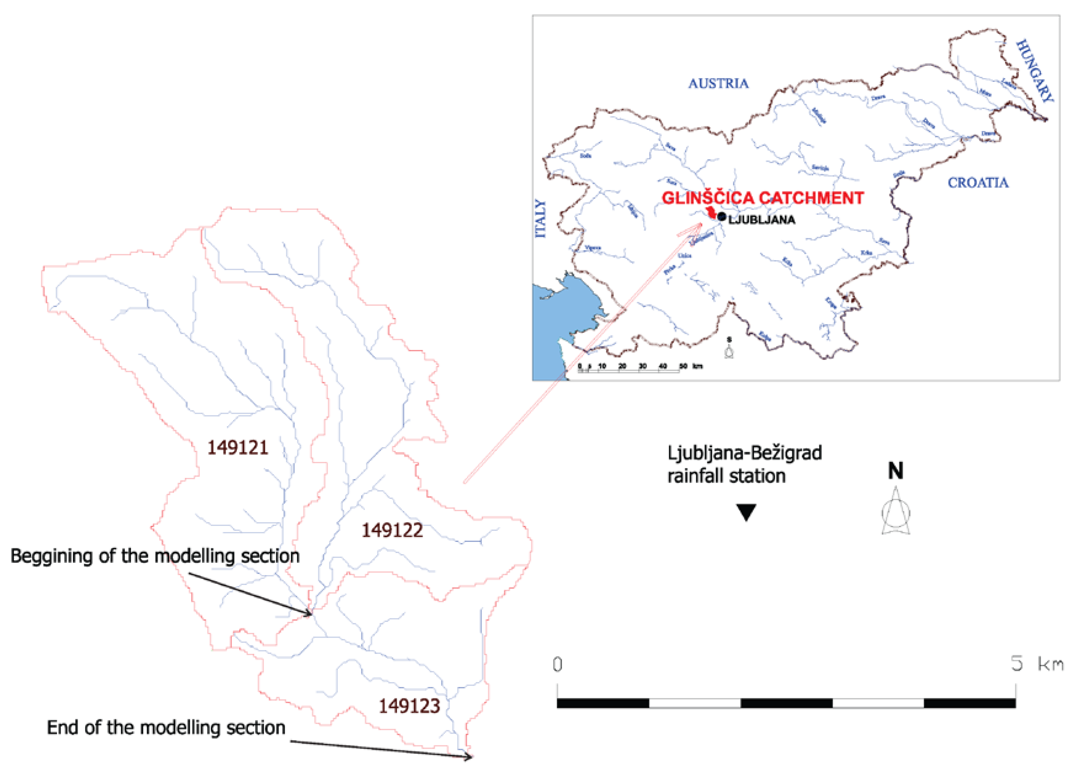
Therefore, the main aim of this study is to explore the relationship between the design hyetograph definition, and hydraulic modelling results. For this purpose, the Glinščica Stream catchment in central Slovenia was selected as the case study. The specific aims are as follows:
(i)
to quantify the effect of rainfall duration on hydraulic modelling results (e.g., flood extent, floodwater velocities);
(ii)
to quantify the impact of temporal rainfall distribution within a rainfall event on hydraulic modelling results, and
(iii)
to compare the differences between flood modelling results (floodplain extents, velocities, volumes, and water depths) for the events with 10 and 100-year return periods.

2. Data and Methods

2.1. Catchment Description

The Glinščica Stream catchment was selected as the case study in order to investigate the impact of the design rainfall on the hydraulic modelling results. The Glinščica Stream catchment is part of the Gradaščica River catchment that drains into the Ljubljanica River. This river is part of the Sava River catchment; the Glinščica Stream catchment is situated in the central part of Slovenia, and reaches into the eastern part of the urban area of the capital city of Ljubljana (Figure 1). The stream has its source under the southeastern slopes of the hills of Polhograjsko hribovje, and at the village of Podutik, it passes into the flat area of the Ljubljana plain. The topography of the catchment is comprised of hilly areas to the east and west, and a flat plain area in the south. The relief of the Glinščica Stream catchment is diverse, comprising hilly headwater areas, as well as flat plains. The Glinščica Stream catchment is one of the hydrologic experimental catchments in Slovenia [35,36]. Table 1 shows some basic properties of the Glinščica Stream catchment. It has already been studied in some of the previous studies, and a more detailed description of the catchment is provided by Bezak et al., Šraj et al. and Brilly et al. [8,14,37]. The lowland areas of the Gradaščica River, once natural floodplain areas, were partly urbanised in the last couple of decades, which resulted in an elevated flood risk for the area. The last major flood occurred in October 2014, when extensive urbanised areas and more than 1000 houses were flooded.
The official water level and discharge measurements in Slovenia are performed by the Slovenian Environment Agency (ARSO). However, in the Glinščica Stream catchment, there is currently no discharge gauging station (there is about 15 years of data available before 1970, but catchment has significantly changed during the past 50 years [38]; therefore, this data was omitted in this study). For the purpose of the research projects and investigation of hydrological processes in the experimental catchment, the water station, which was equipped with an ultrasonic Doppler instrument (Starflow Unidata 6526 model), was placed in the channel of the Glinščica Stream. However, it was only placed there for the limited period of time [14,37]. This means that design discharges cannot be determined using the frequency analysis approach [5], the use of a different approach is required in order to derive the design values for this catchment.

2.2. Hydrological Model

The hydrological model HEC-HMS [39], with a combination of the design hyetographs [21], was used in the study in order to compute design hydrographs that were further used as inputs to the hydraulic model. Three different methods were applied in order to construct the design hyetograph: namely, the Huff method, the constant intensity method, and the frequency storm method. Descriptions of the applied methods can be found, for example, in Ball, Alfieri et al., Azli and Rao, Dolšak et al. [11,17,20,21]. Calibration and validation of the hydrological model of the Glinščica Stream catchment was performed by Šraj et al. [14] using measured discharge data obtained as part of the work that has been done in order to investigate the impact of changed land use (urbanisation) on the hydrological and biogeochemical processes in the experimental catchment [14,37]. For modelling purposes, the Glinščica Stream catchment was divided into three sub-catchments that are shown in Figure 1. A detailed description of the calibration and validation of the hydrological model is provided by Šraj et al. [14].

2.3. Hydraulic Model

Results of the hydrological modelling were used as inputs to the hydraulic model. Hydraulic modelling was performed from the begging (confluence of sub-catchments 149121 and 149122) to the end of the sub-catchment 149123 (confluence of the Glinščica Stream and the Gradaščica River) (Figure 1). The Glinščica Stream catchment was modelled with hydraulic model HEC-RAS 5.0.3, which enables one-dimensional (1D) and two-dimensional (2D) unsteady and steady flow simulations [40]. The basic characteristics of the Glinščica Stream catchment hydraulic model are shown in Table 2. Figure 2 shows a graphical representation of the hydraulic model extent. The connection between the river channel (1D) and the 2D flow area was defined as a lateral structure, which is one of the options that can be used to connect 1D flow in a river channel with 2D flow on 2D flow areas [40]. The average cell size on 2D flow areas was 25.2 m2 and 25.3 m2 for the right bank and left bank 2D flow areas, respectively (Figure 2). The 2D flow areas were represented by the underlying digital terrain model with a cell size of 1 m × 1 m, which is available for all of Slovenia. The HEC-RAS preprocessor computes several geometric and hydraulic characteristics of each cell face that are important for the hydraulic modelling [40]. The model also includes five bridges that are located in the modelled area [38]. Inflows to the modelled area are indicated with black lines on Figure 2. The upstream boundary condition was the flow hydrograph from catchment 149121 (shown in Figure 1), and the downstream boundary condition was the normal depth and discharge contributions from sub-catchments 149122 and 149123 (shown in Figure 1) were modelled as lateral inflows. Unsteady flow simulations with full momentum equations [40] were used in this study. The computation interval was 20 s, and a 36-h period was considered in simulations. Most of the simulations were computed in less than 10 min. All of the hydraulic parameters in the hydraulic model were kept constant during the simulations of the selected scenarios that are presented in the next sub-section.

2.4. Scenarios (Design Rainfall Events)

In order to evaluate impact of the design rainfall on the hydraulic modelling results, the following 10 scenarios (design rainfall events) were determined and applied as inputs to the hydrological model that was used to compute the flow hydrographs at outflows from individual sub-catchments:
  • Design rainfall was defined based on the 50% (Huff 50%, 6 h), 10% (Huff 10%, 6 h), and 90% (Huff 90%, 6 h) Huff curves with a rainfall duration of 6 h (this duration is approximately equal to the catchment time of concentration);
  • Design rainfall was defined based on the 50% Huff curve with a rainfall duration of 2 h (Huff 50%, 2 h), 12 h (Huff 50%, 12 h), and 24 h (Huff 50%, 24 h);
  • Design rainfall was defined as constant rainfall intensity and rainfall duration of 6 h (Const., 6 h);
  • Design rainfall was defined based on the frequency storm method and peak intensity position at 25% (FreqStorm, peak 25%), 50% (FreqStorm, peak 50%), and 75% (FreqStorm, peak 75%) of rainfall duration.
All 10 scenarios were conducted for rainfall with 10 and 100-year return periods. Thus, in total, 20 different combinations were evaluated and analysed. More information about the methodology used to define the Huff curves [21] and intensity–duration–frequency (IDF) curves that were used in this study is available in Bezak et al. [8]. The Huff and IDF curves from the closest Ljubljana-Bežigrad station (shown in Figure 1) were used. Moreover, also additional information about the frequency storm method that was applied in this study is available in Bezak et al. [8]. This method defines the synthetic design hyetograph using the information from the IDF curves, where for different rainfall durations (e.g., 5 min, 15 min, 1 h, 2 h, 3 h, 6 h) the rainfall amount defined by the IDF curve is used. This approach uses the maximum rainfall amounts of different durations as part of one rainfall event, which is usually not the case in the nature (i.e., there is very low probability that the annual maxima of different rainfall durations occur in the same event). Consequently, application of the frequency storm method often results in higher peak discharge values compared to some other design rainfall definitions (from the engineering perspective, this can be regarded as conservative). The main idea of comparison of different scenarios was to explore the impact of the rainfall duration and temporal rainfall distribution within a rainfall event that was defined using Huff curves that were constructed based on the historical rainfall data for different rainfall durations for several Slovenian stations [21] on the hydraulic modelling results.
For the 10 and 100-year return period events, we compared the maximum floodplain extent area, volume of water flowing on the floodplain areas (selected cross-sections are shown in Figure 3), maximum velocities on floodplains, and outflow hydrographs and maximum water depths for all 10 scenarios.

3. Results and Discussion

3.1. 10-Year Return Period Event

In the first step of the study, we obtained hydraulic modelling results for the 10-year return period. Cases for the selected 10 scenarios were computed, and the results were compared. Figure 4 shows a comparison among the outflow hydrographs for the applied scenarios considering the 10-year return period. It can be seen that rainfall duration has a significant influence on the outflow hydrograph. The scenario that represents the 50% Huff curve with a short rainfall duration of 2 h yields smaller peak discharge values than the scenario applying the same Huff curve with a rainfall duration of 6 h. Also, scenarios with longer rainfall durations and the same Huff curve result in smaller peak discharge values compared to the first scenario (Huff 50%, 6 h), where the rainfall duration is approximately equal to the catchment time of the concentration. This finding is consistent with the results from the previous studies, as Šraj et al. [14] documented, which showed that extending the rainfall duration caused increases in the difference in peak discharge and time-to-peak. Furthermore, also, temporal rainfall distribution within a rainfall event has an important impact on the outflow hydrograph, when comparing rainfall events with the same rainfall duration (6 h) (50%, 10%, and 90% Huff curves, constant rainfall intensity and frequency storm method (25%, 50%, and 75% peak position)). It can be seen that the application of the frequency storm method yields larger peak discharge values than the scenario with 6 h of rainfall duration and the 50% Huff curve and the use of constant rainfall intensity within a rainfall event results in smaller peak discharges than the rainfall duration scenario with the Huff 50% curve over 6 h, which has also been reported by other authors [11,13,14,17]. Alfieri et al. [17] argued that the adoption of any rectangular hyetograph significantly underestimates design hydrograph results. Furthermore, Singh [12] concluded that rainfall patterns with temporal variability result in higher peak discharges than one with constant rainfall intensity. For the same return period, different definitions of the temporal rainfall distribution yield different peak discharge values. Some of these methods that are used to define the temporal rainfall distribution can, from an engineering point of view, be regarded as conservative or not so conservative. For example, using the frequency storm method, one can obtain a design discharge that can be regarded as on the safe side (from the design perspective). On the other hand, the constant intensity method yields smaller peak discharge values. Different results can also be obtained using different Huff curves (e.g., 10%, 50%, or 90%). Moreover, if we do not fix the return period variable, numerous combinations are possible to define the design hyetograph. Thus, there are alternative approaches possible, such as the so-called optional design hyetograph [41]. However, this approach was not tested in this study.
In the next step, we compared maximum flood extents, maximum floodplain velocities, and floodplain volumes calculated from the hydraulic model simulations. Table 3 shows a comparison of these values for the 10 selected scenarios for the 10-year return period. One can notice that design rainfall selection yields more than a 35% difference in the maximum floodplain extent values (Table 3). The minimum extent of the flood was obtained using a scenario with a short rainfall duration of 2 h, and a 50% Huff curve, resulting in minimum hydrograph peak discharge. The maximum flood extent was obtained with the application of a scenario that represents a 90% Huff curve and a rainfall duration of 6 h, resulting in maximum hydrograph peak discharge. We also analysed which land-use types were flooded for these 10 scenarios, because flood damage depends on the flooded land-use types and property values (Table 4). For this purpose, a land use map of Slovenia was used [42]. The results show that the largest changes were associated with meadowland use type, which also covers the largest percent of the flooded area (Table 4). In the case of built areas, the largest extension of flooded areas (6.2 × 10³ m2) was calculated for the 90% Huff curve (6-h rainfall duration) scenario, whereas the smallest flooding extent on the built areas (3.5 × 10³ m2) was calculated for the 50% Huff curve (2 h rainfall duration) scenario. This also means that flood damage would be the largest for the previously mentioned scenario (Huff 90%, 6 h). For the 10-year return period, no flow was obtained for cross-sections 3 and 4, which are located on the 2D flow areas that are shown in Figure 3. This means that these areas were not flooded. Four times higher maximum water velocities were obtained for the scenario with a constant rainfall intensity of 6 h than for the scenario with a short rainfall duration of 2 h and the 50% Huff curve for cross-section 1 on the right bank of the flooded area. The water velocity has an important impact both on the stability of human body, and vehicles in the floodwater [27,28,29,30]. Similarly, also, floodplain volumes for different scenarios differ for an order of magnitude (more than 10 times) (Table 3), which indicates that the design rainfall definition has a significant impact on the simulated floodwater dynamics. Moreover, we have also compared the maximum water depths for defined scenarios for the 10-year return period (Table 5). It can be seen that the 90% Huff curve (6 h of rainfall duration) scenario yielded maximum water depth on the right and left floodplain areas (cross-sections 1 and 2) and the 50% Huff curve (2 h of rainfall duration) scenario resulted in minimum water depths (Table 5).

3.2. 100-Year Return Period Event

We have also applied all 10 scenarios for the 100-year return period. Figure 5 shows a comparison of outflow hydrographs for the considered scenarios for the 100-year return period. Compared to the 10-year event (Figure 4), higher peak discharge values were obtained for all of the scenarios, as expected (Figure 5). Similarly, as for the 10-year return period, the maximum peak discharge value was obtained for the scenario using the frequency storm method, with a peak intensity position at 75% of the rainfall duration. On the other hand, the smallest peak discharge value was calculated for scenario based on the 50% Huff curve and 24 h of rainfall duration. Table 6 shows a comparison among the maximum floodplain water extents for investigated cases. The scenario based on the frequency storm method and a peak position at 75% yielded a floodplain extent that was about twice as large as the scenario that used the 50% Huff curve and 24 h of rainfall duration (Table 6). This means that the difference in the peak discharge value for a factor of 1.4 can result in a floodplain water extent that is more than twice as large (Figure 5 and Table 6). Figure 6 shows a comparison between the scenarios that caused the minimum and maximum floodplain extent for the 100-year return period. We also compared the volume of water flowing through cross-sections 1–4 (Figure 3), and the maximum water velocities through these cross-sections (Table 6 and Table 7). The maximum floodplain water velocities exceed 1.2 m/s, and the differences among the maximum water velocities were more than 10 times for some of the scenarios (Table 7). Similar conclusions can also be made for the volume of water flowing through the different floodplain cross-sections (Table 6 and Table 7). Table 8 shows which land use types were flooded during all of the considered scenarios for the 100-year return period. Similarly, as for the 10-year return period, the largest percentage of the flooded area was meadows. For the built areas, the largest extension of flooded areas (22.4 × 10³ m2) was calculated for the FreqStorm, peak 75% scenario, whereas the smallest flooding extent over the built areas (8.1 × 10³ m2) was calculated for the Huff 50%, 24-h scenario. Differences in the design rainfall resulted in a changed extension of the flooded built areas by a factor of 2.8. This poses huge uncertainty in predictions of the maximum flood extent (e.g., for a decision-maker). Further, the uncertainty in flood extent makes it difficult to assess potential flood damages (e.g., by using depth–damage curves), or plan future changes in land use in the flood hazard areas. Moreover, Table 9 shows a comparison between the maximum water depths for different scenarios for the 100-year return period. While the difference between the maximum and minimum water levels at the selected cross-sections seems small (in the range of 6–8 cm), it is well known that small changes in the shallow overflooding depth in urban areas can considerably increase the direct and indirect damage on buildings and urban infrastructure [43]. A review of flood damage studies revealed that that the variation in flood damage to properties could not be explained by inundation depth alone, and should be combined with other factors [44], such as water flow velocity. However, the results of our study show that the water velocities at the selected flood plain cross-sections can vary by a factor of 10.

4. Conclusions

This study presents combined hydrological and hydraulic modelling results for the Glinščica Stream catchment in Slovenia, which can be regarded as a small-scale catchment (less than 20 km2) that is ungauged in terms of discharges. This means that approaches suitable for ungauged catchments are the only option in order to derive design hydrographs, and more specifically design peak discharge values. This study evaluates 10 different design rainfall events (scenarios) that were used as input to the hydrological model. Both 10 and 100-year return period events were analysed. By using calibrated and validated hydrological models, the inputs for the hydraulic model were determined. Thus, the main aim was to evaluate the influence of the design rainfall selection in terms of the rainfall duration and temporal rainfall distribution defined using Huff curves on the hydraulic modelling results (e.g., shape of the outflow hydrograph, peak discharge values, floodplain water extents, maximum floodplain water velocities, and maximum water depths).
The 10 selected and considered scenarios in the study show that the maximum peak discharge value using different design hyetographs and rainfall durations can be 1.4 times larger than the minimum peak discharge value. At the same time, the maximum floodplain extent can be two times larger than the minimum flood extent, and the maximum floodplain water velocity can be 10 times larger than the minimum floodplain velocity scenarios. This means that design rainfall definition can significantly influence the hydraulic modelling results.
Thus, we recommend that the selection of the design rainfall event should be selected with care, and with the consideration of the typical temporal rainfall distribution of the region, which can be described using the Huff curves. Moreover, in order to select the crucial rainfall duration, an analysis of the past flood events could be useful, with the aim of identifying rainfall characteristics that can result in an extreme flood event, such as duration. In combination with the catchment time of concentration, this could be used to select the rainfall duration.

Acknowledgments

The results of the study are part of the Slovenian national research project J2-7322: “Modelling hydrologic response of nonhomogeneous catchments” and research Programme P2-0180: “Water Science and Technology, and Geotechnical Engineering: Tools and Methods for Process Analyses and Simulations, and Development of Technologies” that are financed by the Slovenian Research Agency (ARRS). We wish to thank the Slovenian Environment Agency (ARSO) for data provision.

Author Contributions

All authors drafted the manuscript and determined the aims of the research; N. Bezak carried out the hydrological and hydraulic calculations; All authors contributed to the manuscript writing and revision.

Conflicts of Interest

The authors declare no conflict of interest.

References

  1. Zorn, M.; Komac, B. Damage caused by natural disasters in Slovenia and globally between 1995 and 2010. Acta Geogr. Slov. 2011, 51, 7–30. [Google Scholar] [CrossRef]
  2. Blöschl, G.; Hall, J.; Parajka, J.; Perdigao, R.A.P.; Merz, B.; Arheimer, B.; Aronica, G.T.; Bilibashi, A.; Bonacci, O.; Borga, M.; et al. Changing climate shifts timing of European floods. Science 2017, 357, 588–590. [Google Scholar] [CrossRef] [PubMed]
  3. Šraj, M.; Menih, M.; Bezak, N. Climate variability impact assessment on the flood risk in Slovenia. Phys. Geogr. 2016, 37, 73–87. [Google Scholar] [CrossRef]
  4. Blöschl, G. Recent advances in flood hydrology—Contributions to implementing the Flood Directive. Acta Hydrotech. 2016, 29, 13–22. [Google Scholar]
  5. Bezak, N.; Brilly, M.; Šraj, M. Comparison between the peaks-over-threshold method and the annual maximum method for flood frequency analysis. Hydrol. Sci. J. 2014, 59, 959–977. [Google Scholar] [CrossRef]
  6. Šraj, M.; Bezak, N.; Brilly, M. Bivariate flood frequency analysis using the copula function: A case study of the Litija station on the Sava River. Hydrol. Process. 2015, 29, 225–238. [Google Scholar] [CrossRef]
  7. Blöschl, G.; Sivapalan, M.; Wagener, T.; Viglione, A.; Savenije, H. Runoff Prediction in Ungauged Basins: Synthesis across Processes, Places and Scales, 1st ed.; Cambridge University Press: Cambridge, UK, 2013; 490p. [Google Scholar]
  8. Bezak, N.; Šraj, M.; Mikoš, M. Design rainfall in engineering applications with focus on the design discharge. In Engineering and Mathematical Topics in Rainfall; InTech Press: London, UK, 2018; ISBN 978-953-51-5562-1. [Google Scholar]
  9. Grimaldi, S.; Petroselli, A.; Serinaldi, F. A continuous simulation model for design-hydrograph estimation in small and ungauged watersheds. Hydrol. Sci. J. 2012, 57, 1035–1051. [Google Scholar] [CrossRef]
  10. El-Jabi, N.; Sarraf, S. Effect of maximum rainfall position on rainfall-runoff relationship. J. Hydraul. Eng. 1991, 117, 681–685. [Google Scholar] [CrossRef]
  11. Ball, J.E. The influence of storm temporal patterns on catchment response. J. Hydrol. 1994, 158, 285–303. [Google Scholar] [CrossRef]
  12. Singh, V.P. Effect of spatial and temporal variability in rainfall and watershed characteristics on stream flow hydrograph. Hydrol. Process. 1997, 11, 1649–1669. [Google Scholar] [CrossRef]
  13. Danil, E.I.; Michas, S.N.; Lazaridis, L.S. Hydrologic modeling for the determination of design discharges in ungauged basins. Glob. NEST J. 2005, 7, 296–305. [Google Scholar]
  14. Šraj, M.; Dirnbek, L.; Brilly, M. The influence of effective rainfall on modeled runoff hydrograph. J. Hydrol. Hydromech. 2010, 58, 3–14. [Google Scholar] [CrossRef]
  15. Sikoroska, A.E.; Seibert, J. Appropriate temporal resolution of precipitation data for discharge modelling in pre-alpine catchments. Hydrol. Sci. J. 2017, 63. [Google Scholar] [CrossRef]
  16. Sikoroska, A.E.; Viviroli, D.; Seibert, J. Effective precipitation duration for runoff peaks based on catchment modelling. J. Hydrol. 2017, 556, 510–522. [Google Scholar] [CrossRef]
  17. Alfieri, L.; Laio, F.; Claps, P. A simulation experiment for optimal design hyetograph selection. Hydrol. Process. 2008, 22, 813–820. [Google Scholar] [CrossRef]
  18. Huff, F.A. Time distribution of rainfall in heavy storms. Water Resour. Res. 1967, 3, 1007–1019. [Google Scholar] [CrossRef]
  19. Bonta, J.V. Development and utility of Huff curves for disaggregating precipitation amounts. Appl. Eng. Agric. 2004, 20, 641–653. [Google Scholar] [CrossRef]
  20. Azli, M.; Rao, R. Development of Huff curves for Peninsular Malaysia. J. Hydrol. 2010, 388, 77–84. [Google Scholar] [CrossRef]
  21. Dolšak, D.; Bezak, N.; Šraj, M. Temporal characteristics of rainfall events under three climate types in Slovenia. J. Hydrol. 2016, 541, 1395–1405. [Google Scholar] [CrossRef]
  22. Huff, F. Time Distributions of Heavy Rainstorms in Illinois; Illinois State Water Survey, State of Illinois Department of Energy and Natural Resources: Champaign, IL, USA, 1990; Circular 173.
  23. Savage, J.T.S.; Pianosi, F.; Bates, P.; Freer, J.; Wagener, T. Quantifying the importance of spatial resolution and other factors through global sensitivity analysis of a flood inundation model. Water Resour. Res. 2016, 52, 9146–9163. [Google Scholar] [CrossRef]
  24. Hall, J.W.; Tarantola, S.; Bates, P.D.; Horritt, M.S. Distributed sensitivity analysis of flood inundation model calibration. J. Hydraul. Eng. 2005, 131, 117–126. [Google Scholar] [CrossRef]
  25. Pestotnik, S.; Hojnik, T.; Šraj, M. Analysis of the possibility of using the distributed two-dimensional model Flo-2D for hydrological modeling. Acta Hydrotech. 2012, 25, 85–103. [Google Scholar]
  26. Pappenberger, F.; Matgen, P.; Beven, K.J.; Henry, J.B.; Pfister, L.; de Fraipont, P. Influence of uncertain boundary conditions and model structure on flood inundation predictions. Adv. Water Resour. 2006, 29, 1430–1449. [Google Scholar] [CrossRef]
  27. Shu, C.W.; Xia, J.Q.; Falconer, R.A.; Lin, B.L. Incipient velocity for partially submerged vehicles in floodwaters. J. Hydraul. Res. 2011, 49, 709–717. [Google Scholar] [CrossRef]
  28. Xia, J.Q.; Falconer, R.A.; Wang, Y.J.; Xiao, X.W. New criterion for the stability of a human body in floodwaters. J. Hydraul. Res. 2014, 52, 93–104. [Google Scholar] [CrossRef]
  29. Milanesi, L.; Pilotti, M.; Ranzi, R. A conceptual model of people’s vulnerability to floods. Water Resour. Res. 2015, 51, 182–197. [Google Scholar] [CrossRef]
  30. Milanesi, L.; Pilotti, M.; Bacchi, B. Using web-based observations to identify thresholds of a person’s stability in a flow. Water Resour. Res. 2016, 52, 7793–7805. [Google Scholar] [CrossRef]
  31. Kreibich, H.; Piroth, K.; Seifert, I.; Maiwald, H.; Kunert, U.; Schwarz, J.; Merz, B.; Thieken, A.H. Is flow velocity a significant parameter in flood damage modelling? Nat. Hazards Earth Syst. Sci. 2009, 9, 1679–1692. [Google Scholar] [CrossRef]
  32. Hagemeier-Klose, M.; Wagner, K. Evaluation of flood hazard maps in print and web mapping services as information tools in flood risk communication. Nat. Hazards Earth Syst. Sci. 2009, 9, 563–574. [Google Scholar] [CrossRef]
  33. Tacnet, J.-M.; Batton-Hubert, M.; Dezert, J. Information fusion for natural hazards in mountains. In Advances and Applications of DSmT for Information Fusion; Smarandache, F., Dezert, J., Eds.; American Research Press: Rehoboth, DE, USA, 2009; Chapter 23; Volume III, pp. 565–659. [Google Scholar]
  34. Tacnet, J.-M.; Batton-Hubert, M.; Dezert, J.; Richard, D. Decision Support Tools for Natural Hazards Management under Uncertainty. In Proceedings of the 12th Congress Interpraevent, Grenoble, France, 23–26 April 2012; pp. 597–608. Available online: http://www.interpraevent.at/palm-cms/upload_files/Publikationen/Tagungsbeitraege/2012_1_597.pdf (accessed on 11 February 2018).
  35. Bezak, N.; Šraj, M.; Rusjan, S.; Kogoj, M.; Vidmar, A.; Sečnik, M.; Brilly, M.; Mikoš, M. Comparison between two adjacent experimental torrential watersheds: Kuzlovec and Mačkov graben. Acta Hydrotech. 2013, 26, 85–97. [Google Scholar]
  36. Šraj, M.; Bezak, N.; Rusjan, S.; Mikoš, M. Review of hydrological studies contributing to the advancement of hydrological sciences in Slovenia. Acta Hydrotech. 2016, 29, 47–71. [Google Scholar]
  37. Brilly, M.; Rusjan, S.; Vidmar, A. Monitoring the impact of urbanisation on the Glinscica stream. Phys. Chem. Earth Part A/B/C 2006, 31, 1089–1096. [Google Scholar] [CrossRef]
  38. Rusjan, S.; Fazarinc, R.; Mikoš, M. River rehabilitation of urban watercourses on the example of the Glinščica River in Ljubljana. Acta Hydrotech. 2003, 21, 1–22. [Google Scholar]
  39. HEC-HMS 3.4. Reference Manual. Available online: http://www.hec.usace.army.mil/software/hec-hms/documentation/HEC-HMS_Users_Manual_3.4.pdf (accessed on 11 February 2018).
  40. HEC-RAS 5.0. Reference Manual. Available online: http://www.hec.usace.army.mil/software/hec-ras/documentation/HEC-RAS%205.0%20Reference%20Manual.pdf (accessed on 11 February 2018).
  41. Nguyen, T.A.; Grossi, G.; Ranzi, R. Design Storm for Mixed Urban and Agricultural Drainage Systems in the Northern Delta in Vietnam. J. Irrig. Drain. Eng. 2016, 142, 4015051. [Google Scholar] [CrossRef]
  42. GERK. Land Use Map of Slovenia. Available online: http://rkg.gov.si/GERK/ (accessed on 11 February 2018).
  43. Penning-Rowsell, E.; Johnson, C.; Tunstall, S.; Tapsell, S.; Morris, J.; Chatterton, J.B.; Green, C. The Benefits of Flood and Coastal Risk Management: A Manual of Assessment Techniques; Middlesex University Press: London, UK, 2005. [Google Scholar]
  44. Hammond, M.J.; Chen, A.S.; Djordjević, S.; Butler, D.; Mark, O. Urban flood impact assessment: A state-of-the-art review. Urban Water J. 2015, 12, 14–29. [Google Scholar] [CrossRef]
Figure 1. Location of the Glinščica Stream catchment on a map of Slovenia, and the Glinščica River catchment divided into three sub-catchments. The hydraulic modelling was performed in the 149123 sub-catchment from the beginning (confluence of sub-catchments 149121 and 149122) to the end (confluence of the Glinščica Stream and the Gradaščica River) of the river network in this sub-catchment.
Geosciences 08 00069 g001
Figure 2. Hydraulic model of the Glinščica Stream catchment with two large 2D flow areas.
Geosciences 08 00069 g002
Figure 3. Selected cross-sections (1–4) on the floodplain areas that were used to compare volumes flowing on the floodplains, maximum water velocities on the floodplains, and maximum water depths.
Geosciences 08 00069 g003
Figure 4. Comparison of outflow hydrographs for 10 selected scenarios for a 10-year return period.
Geosciences 08 00069 g004
Figure 5. Comparison of outflow hydrographs for the 10 selected scenarios for the 100-year return period.
Geosciences 08 00069 g005
Figure 6. Comparison between the maximum floodplain extent for scenarios (vi) and (x) indicated with orange and light blue, respectively, for the 100-year return period.
Geosciences 08 00069 g006
Table 1. Basic characteristics of the Glinščica Stream catchment.
Catchment Area (km2)Elevation (m a.s.l.)Land-CoverSoil Characteristics (According to Soil Conservation Service (SCS) Classification)Mean Annual Precipitation (mm)Time of Concentration (h)
16.85from 209 to 59049% forest, 23% agriculture land, 19% urbanised areasC and D types with generally low infiltration ratesabout 1400about 6
Table 2. Basic characteristics of the hydraulic model of the Glinščica Stream catchment. 2D: two-dimensional.
River Length (m)Number of Cross-SectionsNumber of 2D Flow AreasSize of 2D Flow AreasManning’s Roughness Coefficients
about 30009320.64 km2 (left) and 0.50 km2 (right)Between 0.02 to 0.033 for the river channel, 0.04 for the flood area within the cross-section, and between 0.06 and 0.1 for the 2D flood area
Table 3. Comparison among maximum floodplain extents, maximum floodplain velocities, and floodplain volumes for 10 selected scenarios for the 10-year return period. Bold values indicate maximum values in each column.
ScenarioMaximum Flood Water Extent (103 m2)Volume of Water Flowing through Cross-Section 1 (103 m3)Maximum Velocities at Cross-Section 1 (m/s)Volume of Water Flowing through Cross-Section 2 (103 m3)Maximum Velocities at Cross-Section 2 (m/s)
Huff 50%, 6 h89.34.20.212.40.17
Huff 10%, 6 h97.14.70.343.10.19
Huff 90%, 6 h101.16.70.202.50.19
Huff 50%, 2 h65.40.50.091.10.15
Huff 50%, 12 h80.73.10.142.50.15
Huff 50%, 24 h72.92.30.182.00.14
Const., 6 h79.81.90.462.10.16
FreqStorm, peak 25%92.94.00.202.40.20
FreqStorm, peak 50%99.55.50.412.80.19
FreqStorm, peak 75%100.75.80.453.50.19
Table 4. Area (103 m2) of flooded land use types for 10 scenarios for the 10-year return period.
Land Use/ScenarioHuff 50%, 6 hHuff 10%, 6 hHuff 90%, 6 hHuff 50%, 2 hHuff 50%, 12 hHuff 50%, 24 hConst., 6 hFreqStorm, Peak 25%FreqStorm, Peak 50%FreqStorm, Peak 75%
Field15.717.117.611.213.912.514.016.417.417.5
Meadow55.260.663.438.349.343.848.557.762.363.3
Trees and bushes1.41.51.61.01.31.21.31.41.61.6
Uncultivated agriculture land0.00.00.00.00.00.00.00.00.00.0
Forest0.60.80.90.00.60.40.40.70.90.9
Built areas5.25.86.23.54.33.74.45.46.06.1
Water11.311.311.311.311.311.311.311.311.311.3
Table 5. Comparison of maximum water depths for cross-sections 1 and 2 for different scenarios for the 10-year return period.
ScenarioMaximum Water Depth at Cross-Section 1 (m)Maximum Water Depth at Cross-Section 2 (m)
Huff 50%, 6 h0.250.49
Huff 10%, 6 h0.300.56
Huff 90%, 6 h0.330.59
Huff 50%, 2 h0.110.26
Huff 50%, 12 h0.220.47
Huff 50%, 24 h0.180.39
Const., 6 h0.200.41
FreqStorm, peak 25%0.280.51
FreqStorm, peak 50%0.320.57
FreqStorm, peak 75%0.330.59
Table 6. Comparison among maximum floodplain extents, maximum floodplain velocities, and floodplain volumes (cross-sections 1 and 2) for the 10 selected scenarios for the 100-year return period. Bold values indicate the maximum values in each column.
ScenarioMaximum Flood Water Extent (103 m2)Volume of Water Flowing through Cross-Section 1 (103 m3)Maximum Velocities at Cross-Section 1 (m/s)Volume of Water Flowing through Cross-Section 2 (103 m3)Maximum Velocities at Cross-Section 2 (m/s)
Huff 50%, 6 h203.723.80.256.10.26
Huff 10%, 6 h243.625.90.276.90.29
Huff 90%, 6 h245.227.20.266.70.26
Huff 50%, 2 h144.515.70.314.50.24
Huff 50%, 12 h149.128.30.695.90.22
Huff 50%, 24 h134.738.20.187.00.20
Const., 6 h165.321.50.645.00.24
FreqStorm, peak 25%237.427.10.265.30.28
FreqStorm, peak 50%271.829.70.276.80.27
FreqStorm, peak 75%279.928.30.287.20.28
Table 7. Comparison among maximum floodplain velocities and floodplain volumes (cross-sections 3 and 4) for different scenarios for the 100-year return period. Bold values indicate the maximum values in each column.
ScenarioVolume of Water Flowing through Cross-Section 3 (103 m3)Maximum Velocities at Cross-Section 3 (m/s)Volume of Water Flowing through Cross-Section 4 (103 m3)Maximum Velocities at Cross-Section 4 (m/s)
Huff 50%, 6 h8.00.542.60.16
Huff 10%, 6 h11.90.645.00.44
Huff 90%, 6 h11.40.494.81.38
Huff 50%, 2 h2.70.750.60.13
Huff 50%, 12 h5.20.931.20.13
Huff 50%, 24 h3.80.320.80.12
Const., 6 h5.30.841.10.14
FreqStorm, peak 25%10.60.674.10.44
FreqStorm, peak 50%13.70.416.50.46
FreqStorm, peak 75%14.80.537.10.45
Table 8. Area (103 m2) of flooded land use types for the 10 selected scenarios for the 100-year return period.
Land Use/ScenarioHuff 50%, 6 hHuff 10%, 6 hHuff 90%, 6 hHuff 50%, 2 hHuff 50%, 12 hHuff 50%, 24 hConst., 6 hFreqStorm, Peak 25%FreqStorm, Peak 50%FreqStorm, Peak 75%
Field41.552.752.521.722.720.329.150.259.862.1
Greenhouse0.00.10.10.00.00.00.00.30.30.8
Orchard4.410.210.20.00.00.00.09.610.710.8
Meadow112.6128.7130.291.694.888.499.2126.3140.7144.2
Trees and bushes4.15.95.92.42.42.22.75.56.97.2
Uncultivated agriculture land16.218.218.57.17.63.111.618.119.019.1
Forest1.41.51.61.31.31.21.31.51.92.0
Built areas12.214.915.19.19.18.110.114.621.222.4
Water11.311.311.311.311.311.311.311.311.311.3
Table 9. Comparison of maximum water depths for cross-sections 1 and 2 for different scenarios for the 100-year return period.
ScenarioMaximum Water Depth at Cross-Section 1 (m)Maximum Water Depth at Cross-Section 2 (m)
Huff 50%, 6 h0.520.80
Huff 10%, 6 h0.570.84
Huff 90%, 6 h0.570.85
Huff 50%, 2 h0.460.75
Huff 50%, 12 h0.470.75
Huff 50%, 24 h0.450.73
Const., 6 h0.490.77
FreqStorm, peak 25%0.570.84
FreqStorm, peak 50%0.600.86
FreqStorm, peak 75%0.600.86

