Generation of Persistent Scatterers in Non-Urban Areas: The Role of Microwave Scattering Parameters


1
Consiglio Nazionale delle Ricerche, Istituto per le Applicazioni del Calcolo, Via Amendola 122/O, 70126 Bari, Italy
2
Centre for Geographical Studies, IGOT—Institute of Geography and Spatial Planning, Universidade de Lisboa, Edifício IGOT, Rua Branca Edmée Marques, 1600-276 Lisboa, Portugal
3
Instituto Dom Luiz, Universidade de Lisboa, Campo Grande, 1749-016 Lisbon, Portugal
*
Author to whom correspondence should be addressed.
Geosciences 2018, 8(7), 269; https://doi.org/10.3390/geosciences8070269
Submission received: 17 June 2018
/
Revised: 17 July 2018
/
Accepted: 19 July 2018
/
Published: 23 July 2018
(This article belongs to the Special Issue Quantitative Geomorphology)
Abstract
:In this work, we study the capability of the ground surface to generate Persistent Scatterers (PS) based on the lithology, slope and aspect angles. These properties affect the scattering behavior of the Synthetic Aperture Radar (SAR) signal, the interferometric phase stability and, as a consequence, the PS generation. Two-time series of interferometric SAR data acquired by two different SAR sensors in the C-band are processed to generate independent PS datasets. The region north of Lisbon, Portugal, characterized by sparse vegetation and lithology diversity, is chosen as study area. The PS frequency distribution is obtained in terms of lithology, slope and aspect angles. This relationship could be useful to estimate the expected PS density in landslide-prone areas, being lithology, slope and aspect angles important landslide predisposing factors.
1. Introduction
The use of Synthetic Aperture Radar (SAR) data to measure ground displacements was demonstrated in many papers (e.g., see [1] and references therein). A pair of interferometric SAR images, corrected for topography and orbit errors [2] and mitigated for atmospheric phase delay artifacts [3], provides a map of terrain displacements. The number and quality of measurement points on this map depends on the coherence of the two SAR images acquired at two spatially and/or temporally separated antennas.
In this paper, we investigate the ground factors which can increase the interferometric coherence when processing times-series of SAR images by advanced SAR interferometry (InSAR) techniques [4,5,6,7,8] and, as a consequence, the number of measurement points of ground displacements. It was observed that, even in scenes characterized by bare soil, so without apparent decorrelation, the number of measurement points is not spatially uniform and seems to be related to ground morphometry (slope and aspect) and lithology. Vegetation and agricultural practices destroy the temporal interferometric coherence and, as a consequence, reduce the number of measurement points.
For this reason, in this paper we focus on temporal coherent ground surfaces not affected by heavy decorrelation phenomena such as those related to agriculture practice and/or huge vegetation, and study how lithology, ground morphology and geometry can preserve the interferometric coherence and increase the number of measurement points.
In this work, we use the Persistent Scatterers (PS) approach [4,5,6] since it is more effective to identify displacements of relatively small targets such as landslides with respect to Small Baseline (SBAS) [7] and Distributed Scatterers (DS) [8] approaches. Among PS techniques we chose Hooper’s algorithm [6]. This method detects pixels in stacked interferograms characterized by a stable interferometric phase overcoming many of the problems of previous amplitude-based approaches proposed to process a stack of SAR interferograms [4,5]. It was demonstrate that Hooper’s algorithm is effective also when used in non-urban areas [6].
The property of being a PS is related to the ground scattering property of giving a point-like signature even if not necessarily corresponding to point-like targets [6]. The PS techniques can provide a useful and cheap means for the detection and identification of geological phenomena such as landslides and subsidence. They are also useful for monitoring purposes and as a further layer of information for spatial analysis and hazard prediction.
The temporal change of the interferometric phase at PS locations represents a ground deformation of the surface occurring at a scale larger than a pixel. Local changes, i.e., occurring within the SAR image pixel, increase the phase noise. The phase stability of a PS depends on the interferometric coherence of the two SAR images.
Loss of coherence over local portions of an interferogram can be related to the existence of areas where disruption phenomena occurred [9]. Franceschetti et al. investigated the influence of the surface scattering properties on the interferometric coherence related to spatial diversity [10]. They modeled the scattering surface by means of a tilted plane with a superimposed roughness whose height profile is a stationary isotropic stochastic process with zero mean and a given autocorrelation function. It was assumed that the electromagnetic parameters of the ground were locally homogeneous at the scale of a pixel on the SAR image. A closed-form relationship was derived between the interferometric coherence, the parameters of the interferometric configuration (spatial baseline, look angle, radar wavelength), terrain geometry and surface roughness [10]. Spatial variations of surface roughness, soil moisture and vegetation conditions over the observed scene cause large variations of both the backscattering coefficient and interferometric coherence. This information was used to distinguish different surface types in InSAR images [10].
We chose as a study area, a region mainly characterized by bare soils and sparse vegetation. Furthermore, for the sake of simplicity, we assume that the terrain roughness and soil moisture can be given in terms of Lithological Units (LUs) [11,12].
We compute the PS frequency distribution among all LUs and for different classes of terrain slope and aspect angles. The aim of this work is to study the statistical relationship among LUs, slope and aspect class, and the spatial density PS points in ideal interferometric conditions, i.e., in areas not heavily affected by vegetation or other decorrelating effects. For this reason, we selected as a study area a region with a low density of buildings and man-made structures.
The outcome of this work can be useful to predict potentiality and limitations of spaceborne InSAR when proposed as a means to provide displacement maps for landslide inventories [13] in a region with known lithology and ground morphometry.
2. Method
This section describes the proposed methodology to relate the spatial distribution of PS to the ground morphometry and surface scattering parameters. The PS techniques identify coherent radar targets characterized by high phase stability over the time scale covered by the InSAR time series. These targets often correspond to man-made structures, boulders and outcrops and are used as measurement points of ground displacement.
The density of these measurement points depends on the scattering properties of ground surface and the acquisition parameters of the InSAR time series. A SAR interferogram is generated by combining the coherent electromagnetic fields received at two spatially and/or temporally separated antennas.
The coherence is defined as the magnitude of the complex correlation coefficient of the electromagnetic fields backscattered by the illuminated resolution element. This coefficient depends on the variances and covariance of the two electromagnetic fields. The interferometric coherence is directly related to the temporal stability of the surface microwave scattering properties. The backscattered fields at the two antennas were evaluated using the Physical Optics approximation [10].
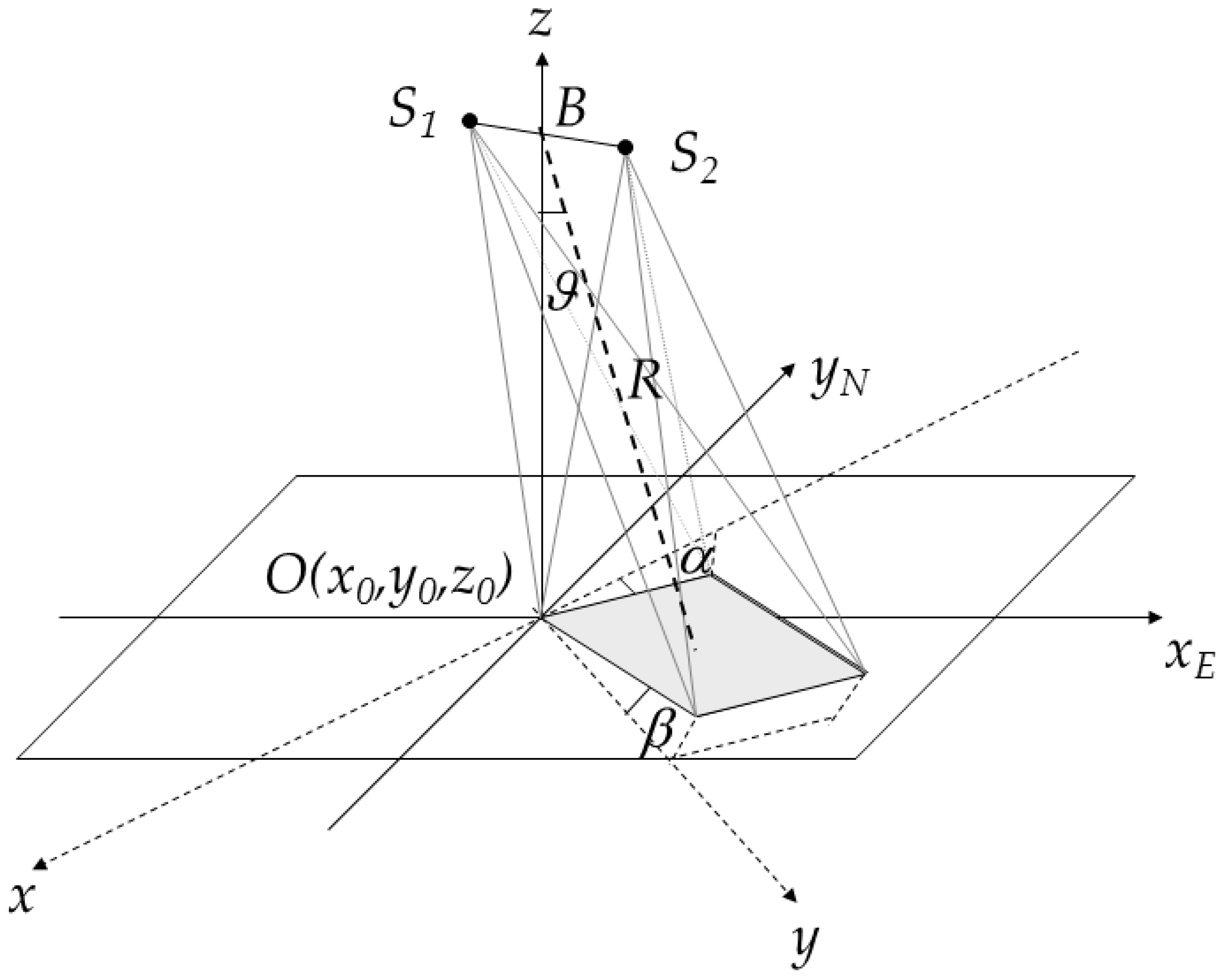
Figure 1 depicts a typical interferometric SAR configuration in both geographical {xE, yN} and SAR {x, y} coordinates. Radar antennas in S1 and S2 points illuminate the ground surface, shown in gray, corresponding to the same pixel on the co-registered SAR images. The variables ϑ, R and ξ give, respectively, the mean radar look angle, the range distance between the spaceborne SAR interferometer and the ground and the satellite track angle. This is modelled as a rough planar surface
where x and y are, respectively, the azimuth and ground-range directions, α and β are the slope angles in the azimuth and ground-range directions, and ε(x, y) is the surface roughness.
Generally, the ground roughness is statistically characterized as a Gaussian surface in terms of the self p(ε) and joint p(ε,ε’) probability density functions, and the normalized autocorrelation function C(τ) is defined as follows
where σ and T are the height standard deviation and the autocorrelation length of the terrain roughness. The correlation coefficient is defined in terms of the scattered electromagnetic fields E1 and E2 as
Computing these fields using the Kirchhoff approximation, Franceschetti et al. [10] derived the following equation for the interferometric coherence
where
and M12 and M11 (M22) are the Hankel transforms, respectively, of the joint and self-characteristic functions of ε and ε’ [10]. Hence, the interferometric coherence is obtained as a function of terrain slope S and aspect A angles, by substituting the values of α and β derived from the following Equations (8) and (9) (see Appendix A for details) in (4)–(7)
where
A total amount of 29 ERS (European Remote Sensing) and 14 ENVISAT (Environmental Satellite) SAR images were processed using the DORIS (Delft object-oriented radar interferometric software) software [2]. Table 1 summarizes the properties of the two time-series and the corresponding time period. The spatial grid of master images were geolocated [14]. The StaMPS (Stanford Method of PS) software was used to identify the PS [6].
The Portugal’s National Laboratory of Energy and Geology made available lithological data at the 1:50,000 scale. This information is mapped in terms of geological formations age. In order to focus on just lithology without taking into account the age of geological formations, 25 different LUs were defined [12]. A LU represents a given combination of geological formations even of different ages sharing a similar lithology. The concept of LUs has great relevance when characterizing the mechanical properties of materials and here it is used as a characterization of the terrain roughness when interpreting phase stability properties of InSAR signal scattered by those materials.
A recent (20 m cell size) Digital Terrain Model (DTM) with a nominal vertical accuracy of 2.5 m was used to derive the terrain slope and aspect angles. Slope and aspect angles were computed, respectively, in classes of 5° and 45°. The study area is mainly characterized by a gentle relief (about 80% of the area has slopes smaller than 15°) and has a small predominance of south exposure.
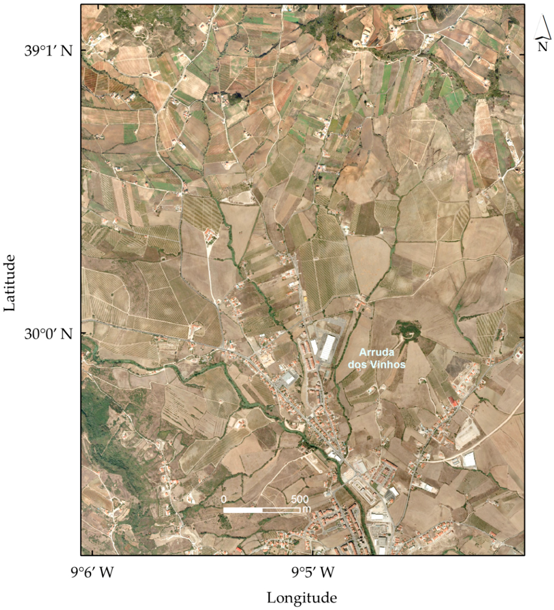
An updated database with information about buildings and the larger man-structures were used to derive a binary mask. A buffering of 20 m was applied to all infrastructures. It was found that about 12% of the study area is covered by buildings and man-made structures. The area is mainly characterized by bare or sparsely vegetated soils. Figure 2 gives an example of the typical vegetation cover in the study area which mainly consists of cultivated areas.
3. Geological and Geomorphological Settings
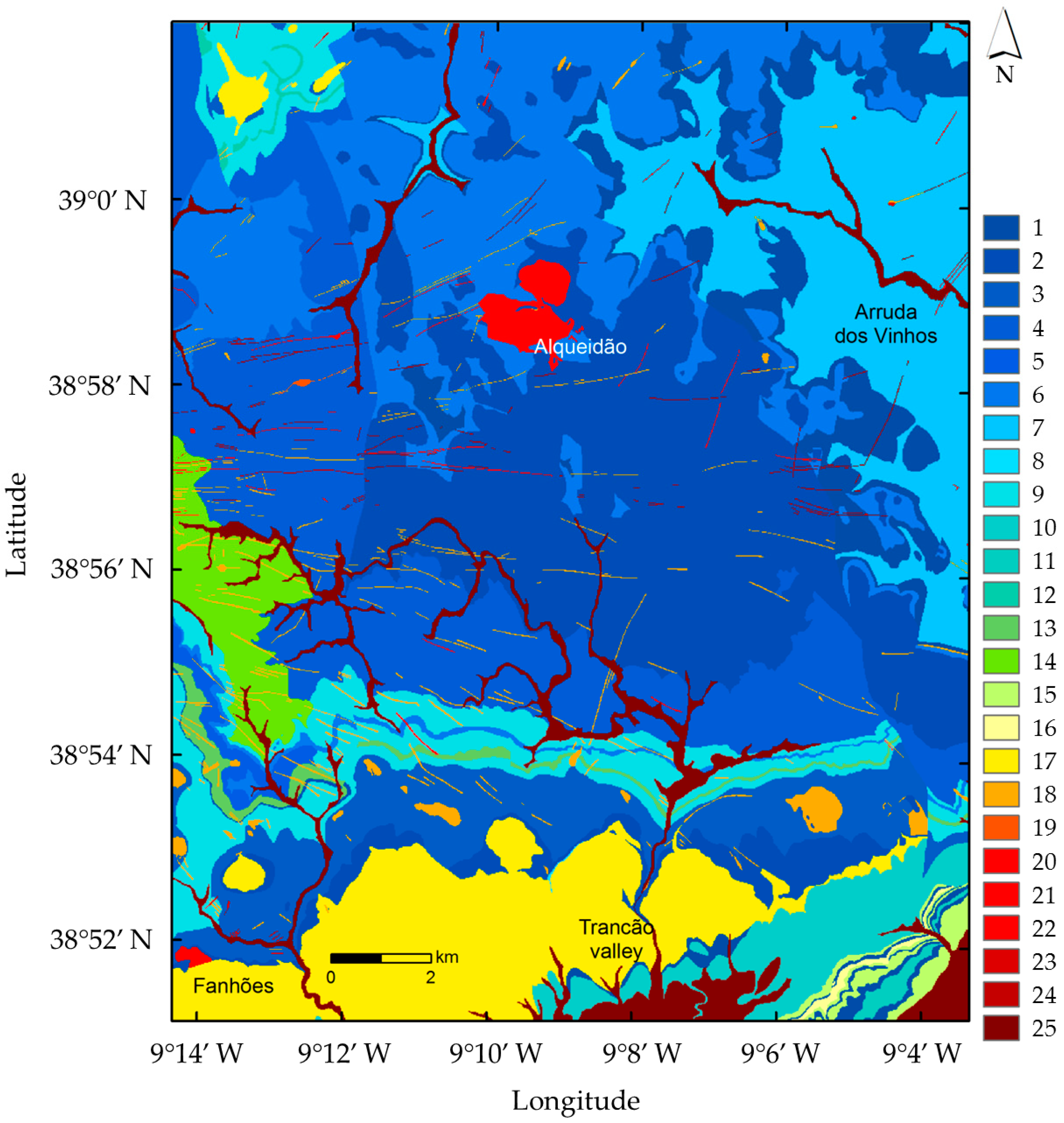
The study area encompasses the regions of Arruda dos Vinhos and Fanhões Trancão/Lousa (north of Lisbon, Portugal) and extends over 320 km2. Figure 2 displays an orthophoto of the study area, characterized by sparse vegetation which facilitates the SAR interferometry analysis. Figure 3 shows the lithological maps of the study area. All LUs are summarized in Table 2. However, it is also possible to discriminate within a LU the relative weight of each lithological type. For instance, in the case of LU # 2 (limestones and marls) the order of lithological units means that limestones are more abundant than marls. Hence, LUs from # 1 to # 6 are all characterized by an overwhelming presence of limestones. This “hierarchy” has a great relevance when the mechanical properties of materials are taken into account or when interpreting phase stability properties of InSAR signals scattered by those materials. The elevation ranges from 440 m at Alqueidão (teschenite batholith intrusion, LU 21 as shown in Figure 3) and 0 m in the southeast sector of the study area (Tagus river alluvial plain, LU 25 as shown in Figure 3).
The LUs present in the study area are mainly sedimentary and heterogeneous (sandstone, conglomerates, limestones, marls and mudstones), dated from the Jurassic and Cretaceous periods. Lithological units are progressively more recent from the north to the south/southeast sector of the study area where tertiary (Eocene and Miocene) and quaternary (Pleistocene fluvial terraces and Holocene alluviums, LU 25) lithologies can be found [12,15]. This sedimentary sequence also includes an upper cretaceous extensive volcanic formation of basalts and volcanic tuffs (LU 17). The study area’s structural characteristics reflect the compressive tectonic deformation that Jurassic and Cretaceous materials suffered during the Upper Miocene [16] producing large ENE-WSW synclines and anticlines north of the Lisbon region. In the northeast sector of the study area a gentle positive tectonic curvature deformation centered in Arruda dos Vinhos with gentle bedding planes, dipping outwards the basin center, controls the study area geological structure [12,16]. In the study area, differential erosion prevailed during the Quaternary [17] promoting the development of large erosive depressions, the Arruda dos Vinhos depression in the northeast sector of the study area (relief inversion) and the Loures depression to south of the Trancão valley. To the south of the Arruda dos Vinhos erosive depression, the monoclinal structure, with layers dipping 5° to 25° towards the south and southeast promote the development of a “cuestas” relief forming asymmetric slopes (e.g., see [18]). These regional geomorphological settings are controlled by the alternation of rocks with different mechanical, erosion, permeability and plasticity properties and by a geological structure favourable to slope instability. In this study area were registered from 1958 up to 2010, 25 rainfall-triggered landslide events (e.g., see [19]). Regional landslide activity is marked by the occurrence of shallow soil slips (depth of the rupture surface less than 1.5 m) and deep-seated landslides (translational and rotational slides and complex landslides with typical depth of the rupture surface from 3 to 5 m). A large number of landslides were identified and mapped at the scale 1:2000 through detailed field geomorphological mapping or by aerial photography interpretation (e.g., [11,20,21]), particularly in: (i) LU17—Upper Cretaceous Volcanic Complex of Lisbon (basalts and volcanic tuffs); LU3—Albian-Cenomanian limestones and sandstones; LU2 and LU4—Upper Jurassic limestones marls and sandstones; and LU7—Upper Jurassic marls and mudstones.
4. Results and Discussion
In this section, we present the results of the analysis of PS’ estimated over the study area, characterized by bare soils and sparse vegetation. A binary mask was built to discriminate PS generated by man-made structure’s natural ground surfaces. Table 3 summarizes the results of this analysis. It gives the number (and fraction) of PS corresponding to man-made structures and bare or sparsely vegetated soils.
The location of PS’ is displayed in Figure 4 with blue and red dots giving, respectively, building and bare soil related PS’. The spatial density of PS varied from 16 PS per-squared-km in the ERS 1992–1997 time series to 25 in the ENVISAT 2003–2005 time series.
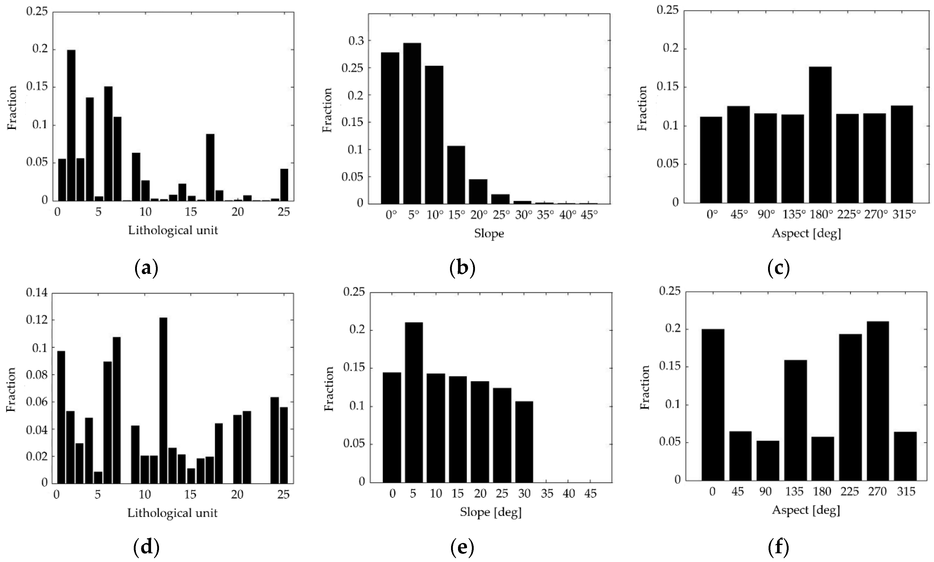
The largest spatial density of PS’ and the fraction of those corresponding to bare or sparsely vegetated soil were found in the time series 2003–2005, elapsing the shortest time interval and containing only 14 SAR images. In contrast, in the time series 1992–1997, the smaller spatial density and the largest fraction of PS related to buildings were found. Figure 5 shows, from the top to the bottom and from the left to the right, the frequency distributions of LU, slope and aspect classes and the PS frequency distributions in terms of lithology, slope and aspect angles, normalized to the area of LU classes for the ERS time series.
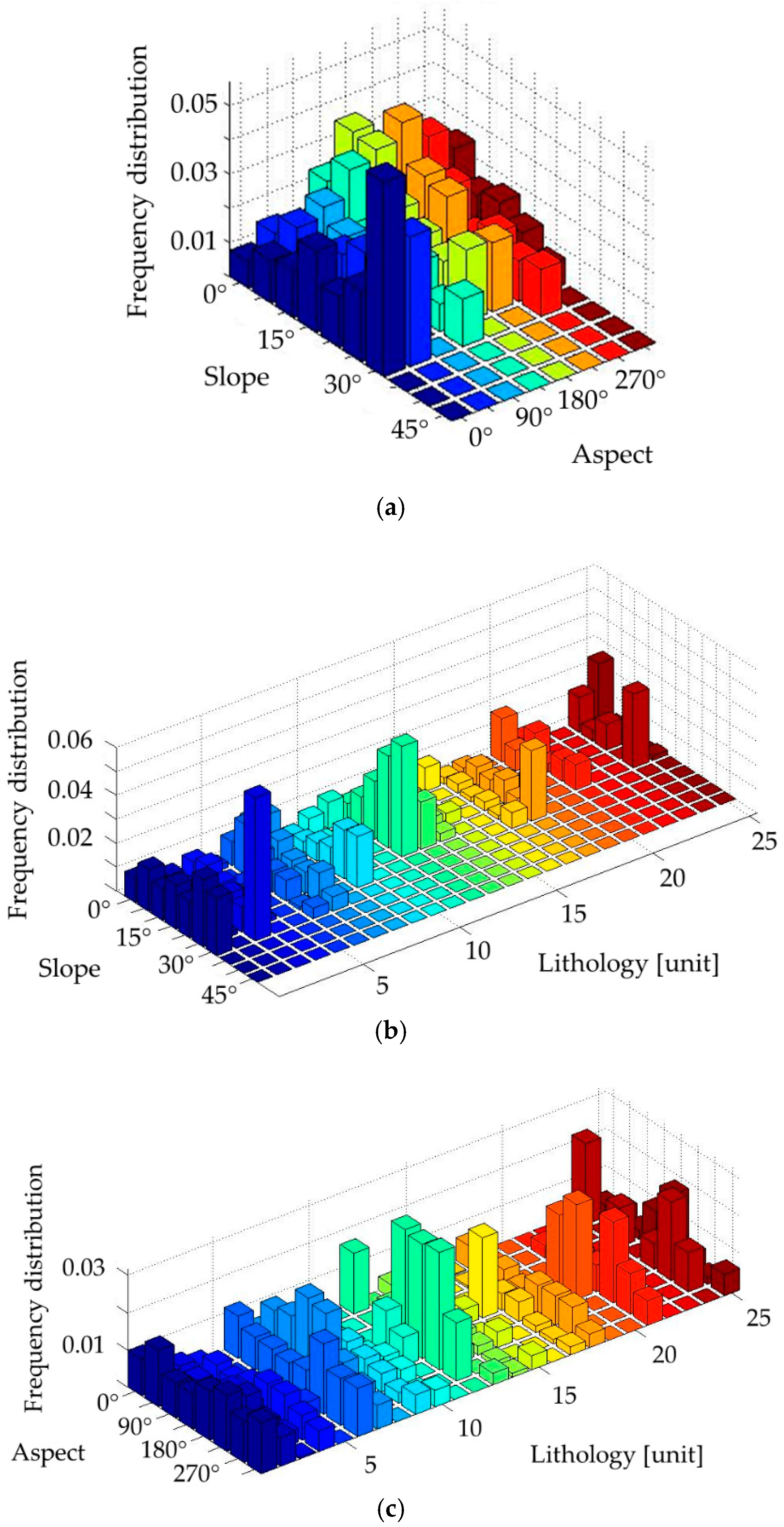
As far as the relationship between PS and LU is concerned, it was found that the largest fractions of PS’ were generated over area with LUs 1, 6, 7 and 12 (see Table 2). These LUs are characterized by the presence of limestones (LUs 1 and 6) or sandstones (LUs 7 and 12). It is worth noting that even if just a negligible fraction of the study area is characterized by the LU 12 (see Figure 5a), a large PS density was found in correspondence of this LU (see top-left of Figure 5d). This can be explained by the presence of sandstones, in some cases it is very resistant to differential erosion, shaping a terrain roughness prone to scatter a PS-like signal. As far as the slope angle is concerned, it was observed that terrain slopes steeper than 35° did not generate PS’ even if in the study area there were slopes up to 50° and more. Furthermore, it was found that the slope class more prone to generate PS’ was that from 5° to 10°. Instead, the aspect classes more prone to PS generation were from 0° to 45° (N), from 135° to 180° (SE) and from 225° to 315° (SW to NW). These results can be explained in terms of the SAR observation geometry and terrain exposure. In fact, all SAR images were acquired along a descending orbit. As a consequence, slopes exposed to the north and east have more favourable imaging conditions and, hence, can generate more PS candidates. However, also slopes exposed to the south (the largest fraction in this area) and west can generate PS if they have small slope angles, in order to avoid shadowing. This observation seems to be confirmed by the PS frequency distributions as a function of slope and aspect angles, slope angle and lithology, and aspect angle and lithology reported in Figure 6.
5. Conclusions
In this work we studied the properties of PS’ estimated in a non-urban environment characterized by bare soil or sparse vegetation. A statistical analysis was carried out to derive a relationship between PS spatial density, lithology and ground morphometry. As far as lithology is concerned, it was found that limestones and sandstones are more prone to generate PS-like signals in InSAR time series. It was also found that the dependence of PS density on lithology is modulated by the ground morphology. In particular, it was found that slopes steeper than 35° did not generate PS in the study area and that the largest fraction of PS’ was found in the range between 5° and 10°. Also, the slope exposure was found to be important. Depending on the satellite orbit (descending or ascending), some aspect classes generated smallest fractions of PS’ except in areas with small slope angles. Furthermore, it was found that shortest InSAR time series gave the largest PS spatial density. This means that, for a given number of SAR images, spaceborne missions with the shortest revisiting cycles, as the current mission Sentinel-1 of the European Space Agency, provide the largest PS spatial densities in non-urban areas. All these considerations could help for a more cost-effective use of a PS-InSAR technique for the monitoring of geological phenomena.
Author Contributions
Conceptualization, G.N. and S.C.O.; Methodology, G.N.; Software, G.N.; Validation, G.N., S.C.O., J.C. and J.L.Z.; Formal Analysis, G.N.; Investigation, G.N. and S.C.O.; Resources, J.C. and J.L.Z; Data Curation, S.C.O.; Writing-Original Draft Preparation, G.N. and S.C.O.; Writing-Review & Editing, G.N. and S.C.O.; Visualization, G.N. and S.C.O.; Supervision, J.C. and J.L.Z..; Project Administration, J.C. and J.L.Z.; Funding Acquisition, J.C. and J.L.Z.
Funding
This research was funded by Fundação para a Ciência e a Tecnologia, Portugal (FCT). Sérgio C. Oliveira has a Postdoctoral Grant (SFRH/BPD/85827/2012) funded by Fundação para a Ciência e a Tecnologia, Portugal (FCT).
Acknowledgments
This work was supported by the project BeSafeSlide—Landslide Early Warning soft technology prototype to improve community resilience and adaptation to environmental change (PTDC/GES-AMB/30052/2017).
Conflicts of Interest
The authors declare no conflict of interest. The funders had no role in the design of the study; in the collection, analyses, or interpretation of data; in the writing of the manuscript, and in the decision to publish the results.
Appendix A
This appendix deals with the relationship between the terrain slope and aspect angles and the angles α and β, describing the terrain morphology as observed in the radar observation geometry (see Figure 1). Let us start by computing the derivatives of terrain height z with respect to the geographical planar coordinates {xE, yN} as
and
In both cases, the derivatives have been given in terms of the SAR planar coordinates {x,y}, the slope angles α and β of the terrain patch along the azimuth and ground-range directions, and the satellite track angle ξ shown in Figure 1. The terrain slope S and aspect A angles are defined, respectively, as
and
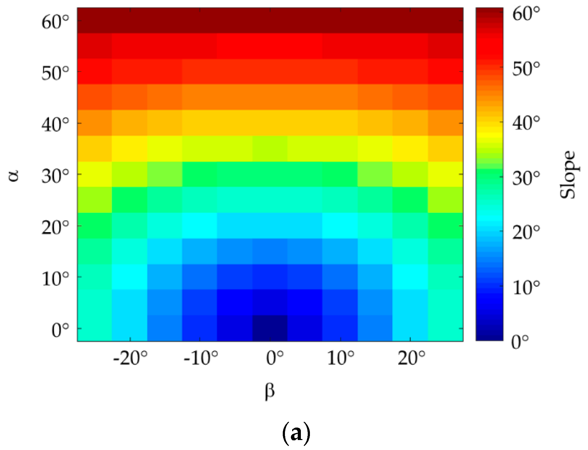
Figure 6 displays the maps of slope and aspect angles as functions of (α, β) whose ranges of values were chosen as suggested by Franceschetti et al. [10]. The satellite track angles were set to ξ = 7°, corresponding to a ERS/Envisat descending orbit. The inversion of Equations (A3) and (A4) results in Equations (9) and (10).
Figure A1.
Terrain slope (a) and aspect (b) values as a function of angles α and β.


References
- Massonnet, D.; Feigl, K.L. Radar interferometry and its application to changes in the Earth’s surface. Rev. Geophys. 1998, 36, 441–500. [Google Scholar] [CrossRef]
- Kampes, B.; Hanssen, R.; Perski, Z. Radar interferometry with public domain tools. In Proceedings of the FRINGE, Frascati, Italy, 1–5 December 2003. [Google Scholar]
- Nico, G.; Tomé, R.; Catalão, J.; Miranda, P.M.A. On the use of the WRF model to mitigate tropospheric phase delay effects in SAR interferograms. IEEE Trans. Geosci. Remote Sens. 2011, 49, 4970–4976. [Google Scholar] [CrossRef]
- Ferretti, A.; Prati, C.; Rocca, F. Permanent scatterers in SAR interferometry. IEEE Trans. Geosci. Remote Sens. 2001, 39, 8–20. [Google Scholar] [CrossRef] [Green Version]
- Lyons, S.; Sandwell, D. Fault creep along the southern San Andreas from interferometric synthetic aperture radar, permanent scatterers and stacking. J. Geophys. Res. 2003, 108, 2047. [Google Scholar] [CrossRef]
- Hooper, A.; Zebker, H.; Segall, P.; Kampes, B. A new method for measuring deformation on volcanoes and other natural terrains using In-SAR persistent scatterers. Geophys. Res. Lett. 2004, 31, L23611. [Google Scholar] [CrossRef]
- Berardino, P.; Fornaro, G.; Lanari, R.; Sansosti, E. A new algorithm for surface deformation monitoring based on small baseline differential SAR interferograms. IEEE Trans. Geosci. Remote Sens. 2002, 40, 2375–2383. [Google Scholar] [CrossRef]
- Ferretti, A.; Fumagalli, A.; Novali, F.; Prati, C.; Rocca, F.; Rucci, A. A new algorithm for processing interferometric data-stacks: SqueeSAR. IEEE Trans. Geosci. Remote Sens. 2011, 49, 3460–3470. [Google Scholar] [CrossRef]
- Gabriel, A.K.; Goldstein, R.M.; Zebker, H. Mapping small elevation changes over large areas differential radar interferometry. J. Geophys. Res. 1989, 94, 9183–9191. [Google Scholar] [CrossRef]
- Franceschetti, G.; Iodice, A.; Migliaccio, M.; Riccio, R. The effect of surface scattering on IFSAR baseline decorrelation. J. Electromagn. Waves Appl. 1987, 11, 353–370. [Google Scholar] [CrossRef]
- Oliveira, S.C.; Zêzere, J.L.; Catalão, J.; Nico, G. The contribution of PSInSAR interferometry to landslide hazard in weak rock-dominated areas. Landslides 2015, 12, 703–719. [Google Scholar] [CrossRef]
- Zbyszewski, G.; Assunção, C.T. Notícia Explicativa da Folha 30-D (Alenquer); Carta Geológica de Portugal; Serviços Geológicos de Portugal: Lisboa, Portugal, 1965. [Google Scholar]
- Righini, G.; Pancioli, V.; Casagli, N. Updating landslide inventory using Persistent Scattering Interferometry (PSI). Int. J. Remote Sens. 2012, 33, 2068–2096. [Google Scholar] [CrossRef]
- Nico, G. Exact-closed form geolocation for SAR intrerferometry. IEEE Trans. Geosci. Remote Sens. 2002, 40, 220–222. [Google Scholar] [CrossRef]
- Kullberg, J.; Rocha, R.; Soares, A.; Rey, J.; Terrinha, P.; Callapez, P.; Martins, L. A Bacia Lusitaniana: Estratigrafia, paleogeografia e tectónica. In Geologia de Portugal no Contexto da Ibéria; Dias, R., Araújo, A., Terrinha, P.M., Kullberg, J., Eds.; Universidade de Évora: Évora, Portugal, 2006; pp. 317–368. [Google Scholar]
- Ribeiro, A.; Antunes, M.T.; Ferreira, M.P.; Rocha, R.B.; Soares, A.F.; Zbyszewski, G.; De Moitinho Almeida, F.; Carvalho, D.; Monteiro, J.H. Introduction à la Géologie Générale du Portugal; Serviços Geológicos de Portugal: Lisboa, Portugal, 1979. [Google Scholar]
- Zêzere, J.L.; Trigo, R.M.; Fragoso, M.; Oliveira, S.C.; Garcia, R.A.C. Rainfall-triggered landslides in the Lisbon region over 2006 and relationships with North Atlantic Oscillation. Nat. Hazards Earth Syst. Sci. 2008, 8, 483–499. [Google Scholar] [CrossRef]
- Zêzere, J.L.; Garcia, R.A.C.; Oliveira, S.C.; Reis, E. Probabilistic landslide risk analysis considering direct costs in the area north of Lisbon (Portugal). Geomorphology 2008, 94, 467–495. [Google Scholar] [CrossRef]
- Zezere, J.L.; Vaz, T.; Pereira, S.; Oliveira, S.C.; Marques, R.; Garcia, R. Rainfall thresholds for landslide activity in Portugal. Environ. Earth Sci. 2015, 73, 2917–2936. [Google Scholar] [CrossRef]
- Zêzere, J.L.; Reis, E.; Garcia, R.; Oliveira, S.; Rodrigues, M.L.; Vieira, G.; Ferreira, A.B. Integration of spatial and temporal data for the definition of different landslide hazard scenarios in the area north of Lisbon (Portugal). Nat. Hazards Earth Syst. Sci. 2004, 4, 133–146. [Google Scholar] [CrossRef] [Green Version]
- Zêzere, J.L.; Oliveira, S.C.; Garcia, R.A.C.; Reis, E. Landslide risk analysis in the area north of Lisbon (Portugal): Evaluation of direct and indirect costs resulting from a motorway disruption by slope movements. Landslides 2007, 4, 123–136. [Google Scholar] [CrossRef]
Figure 1.
Geometrical configuration of InSAR data acquisition (see text for the definition of variables).
Figure 1.
Geometrical configuration of InSAR data acquisition (see text for the definition of variables).

Figure 2.
Sample of orthophoto acquired over the study area.

Figure 3.
Lithological units map of the study area.

Figure 4.
Location of Persistent Scatterers: ERS 1992–1997 (a) and ENVISAT 2003–2005 (b).

Figure 5.
Normalized frequency distributions of LU units (a), slope (b) and aspect angles (c); normalized frequency distributions of PS (ERS 1992–1997) as a function of lithological units (d) slope (e) and aspect classes (f).
Figure 5.
Normalized frequency distributions of LU units (a), slope (b) and aspect angles (c); normalized frequency distributions of PS (ERS 1992–1997) as a function of lithological units (d) slope (e) and aspect classes (f).

Figure 6.
Frequency distribution of PS (1992–1997) as a function of slope and aspect classes (a), slope class and lithology (b), and aspect class and lithology (c).
Figure 6.
Frequency distribution of PS (1992–1997) as a function of slope and aspect classes (a), slope class and lithology (b), and aspect class and lithology (c).


Table 1.
Summary of the InSAR dataset.
| Sensor | N. of Images | Time Interval | Look Angle | Orbit |
|---|---|---|---|---|
| ERS-1/2 | 29 | 1992–1997 | 23° | Descending |
| ENVISAT | 14 | 2003–2005 | 23° | Descending |
Table 2.
Lithological Units.
| Lithological Unit ID | Lithology | Lithological Unit ID | Lithology |
|---|---|---|---|
| 1 | Limestones | 14 | Sandstones, mudstones, limestones and dolomites |
| 2 | Limestones and marls | 15 | Sand |
| 3 | Limestones and sandstones | 16 | Clays |
| 4 | Limestones, marls and sandstones | 17 | Volcanic complex of Lisbon |
| 5 | Limestones, sandstones and mudstones | 18 | Basalt |
| 6 | Limestones, marls, sandstones and mudstones | 19 | Basalt breccia |
| 7 | Marls and mudstones | 20 | Dolerite |
| 8 | Conglomerate | 21 | Techenite |
| 9 | Conglomerates, sandstones and mudstones | 22 | Riolite |
| 10 | Conglomerates, sandstones and claystones | 23 | Traquite and traqui-basalt |
| 11 | Sandstones | 24 | Weathered or not defined rocks |
| 12 | Sandstones and mudstones | 25 | Alluvium, terrace deposits and anthropogenic terraces |
| 13 | Sandstones, mudstones and dolomites | ||
Table 3.
Number of Persistent Scatterers (total, on man-made structures and bare soil).
| Time Series | NTOT of PS | Man-Made Structures | Bare Soil |
|---|---|---|---|
| 1992–1997 (ERS) | 4756 (100%) | 2027 (43%) | 2729 (57%) |
| 2003–2005 (ENVISAT) | 8003 (100%) | 2734 (34%) | 5269 (66%) |
© 2018 by the authors. Licensee MDPI, Basel, Switzerland. This article is an open access article distributed under the terms and conditions of the Creative Commons Attribution (CC BY) license (http://creativecommons.org/licenses/by/4.0/).
Share and Cite
MDPI and ACS Style
Nico, G.; Oliveira, S.C.; Catalão, J.; Zêzere, J.L. Generation of Persistent Scatterers in Non-Urban Areas: The Role of Microwave Scattering Parameters. Geosciences 2018, 8, 269. https://doi.org/10.3390/geosciences8070269
AMA Style
Nico G, Oliveira SC, Catalão J, Zêzere JL. Generation of Persistent Scatterers in Non-Urban Areas: The Role of Microwave Scattering Parameters. Geosciences. 2018; 8(7):269. https://doi.org/10.3390/geosciences8070269
Chicago/Turabian StyleNico, Giovanni, Sérgio C. Oliveira, Joao Catalão, and José Luis Zêzere. 2018. "Generation of Persistent Scatterers in Non-Urban Areas: The Role of Microwave Scattering Parameters" Geosciences 8, no. 7: 269. https://doi.org/10.3390/geosciences8070269
Note that from the first issue of 2016, this journal uses article numbers instead of page numbers. See further details here.