Article

Bayesian Variable Selection for Pareto Regression Models with Latent Multivariate Log Gamma Process with Applications to Earthquake Magnitudes

1
Department of Statistics, Florida State University, Tallahassee, FL 32306, USA
2
Department of Statistics, University of Connecticut, Storrs, CT 06269, USA
*
Author to whom correspondence should be addressed.
Geosciences 2019, 9(4), 169; https://doi.org/10.3390/geosciences9040169
Submission received: 10 January 2019 / Revised: 3 April 2019 / Accepted: 9 April 2019 / Published: 12 April 2019

Abstract

:
Generalized linear models are routinely used in many environment statistics problems such as earthquake magnitudes prediction. Hu et al. proposed Pareto regression with spatial random effects for earthquake magnitudes. In this paper, we propose Bayesian spatial variable selection for Pareto regression based on Bradley et al. and Hu et al. to tackle variable selection issue in generalized linear regression models with spatial random effects. A Bayesian hierarchical latent multivariate log gamma model framework is applied to account for spatial random effects to capture spatial dependence. We use two Bayesian model assessment criteria for variable selection including Conditional Predictive Ordinate (CPO) and Deviance Information Criterion (DIC). Furthermore, we show that these two Bayesian criteria have analytic connections with conditional AIC under the linear mixed model setting. We examine empirical performance of the proposed method via a simulation study and further demonstrate the applicability of the proposed method in an analysis of the earthquake data obtained from the United States Geological Survey (USGS).

1. Introduction

The earthquake magnitude data has become increasingly popular over the last decade. Statistical models for earthquake have been proposed since 1800s. Since large earthquakes are rare, it is difficult to fit simple linear models. Many different parametric models (Gamma model, Weibull model) have been considered to analyze earthquake magnitudes, but some earthquakes with very small magnitudes are not reported by seismic centers. The Pareto-type distribution is a popular choice for analyzing earthquake magnitudes data (e.g., [1,2,3]), as the Pareto distribution is a heavy-tailed distribution with a lower threshold. In statistical analysis, a regression model is used to connect dependent covariates of earthquakes to the magnitude of the earthquake. A generalized linear model strategy can be used for the Pareto regression. Existing seismology literatures pay less attention to spatially dependent structure on earthquake magnitudes. They just built simple linear regression models or generalized linear models to explore covariates effects on earthquake magnitudes [4]. Hu and Bradley [5] proposed using the Pareto regression with spatial random effects for earthquake magnitudes, but they did not consider the model selection problems. In order to have more explicit understanding of dependent covariates of earthquake magnitudes, variable selection approaches should be considered in a Pareto regression model with spatial random effects.
Variable selection and Bayesian statistics have received widespread attention and become increasingly important tools in the field of environment and ecology [6,7]. For hierarchical spatial model, it is difficult to do inference for latent variables. Bayesian approach provides a convenient way for estimating latent variables in hierarchical models. Compared with the frequentist approach, a Bayesian approach can bring some prior information on parameters of the model. It is an important part of a statistical analysis. In practice, we may want to measure how good a model is for answering a certain question or comparing different models to see which model is best suited. There are many popular variable selection criteria, including Akaike’s information criterion (AIC) [8] and Bayesian information criterion (BIC) [9], Bayes factor, conditional predictive ordinate (CPO) [10,11], L measure [12], and the deviance information criterion (DIC) [13]. Chen et al. [14] provide the connections between these popular criteria for variable subset selection under generalized linear models. However, there are some difficulties for Bayesian variable selection to carry out because of the challenge in assigning prior distributions for the parameters. In order to tackle this issue, we consider the multivariate log-Gamma distribution (MLG) based on Bradley et al. [15], which is conjugate with the Pareto distribution [5]. Hence, the Bayesian approach to variable selection is straightforward for our model. Consequently, we use CPO and DIC criteria to carry out Bayesian variable selection for Pareto regression models due to the performance of the conjugate priors (see [16], for a discussion).
Both CPO and DIC are criteria-based methods and they have some advantage over other criteria. Compared with regularized estimation approach, these two criteria consider goodness of fit of the candidate models. Furthermore, compared with negative log probability density or RMSE for predictions, these two criteria consider the model complexity. Like the AIC or BIC, these two criteria compromise the tradeoff between the goodness of fit and model complexity. The CPO provides a site-specific model fit metric that can be used for exploratory analysis and can be combined at the site to generate a logarithm pseudo marginal likelihood (LPML) as an overall model fit measure. The CPO is based on leave-one-out-cross-validation. It estimates the probability of observing data on one particular location in the future if after having already observed data. The LPML is a leave-one-out cross-validation with log likelihood as the criteria which can be easily obtained from an Markov chain Monte Carlo (MCMC) output (see [17]). More details about two criteria will be discussed in Section 2.2. The major contribution of this paper is that we introduce two Bayesian model selection criteria in generalized linear model with spatial random effects. Furthermore, we exam the relationship between the two criteria with conditional AIC (cAIC) in random effects model. Other than the variable selection problem in regression model, our criteria can also be used in model selection in the presence of spatial random effects. In general, our proposed criteria can select important covariates and random effects model simultaneously.
The remaining sections of this article are organized as follows. Section 2 introduces our proposed statistical model, and review two Bayesian model assessment Criteria including LPML and DIC [13]. In Section 3 and Section 4, we present MCMC scheme and a simulation study for two scenarios, and use two criteria to select true model. In Section 5, we carry out a detailed analysis of the US earthquake dataset from United States Geological Survey (USGS) and use two criteria to select the best model(s). Finally, Section 6 contains a brief summary of this paper. For ease of exposition all proofs are given Appendix A.

2. Methodology

2.1. Pareto Regression with Spatial Random Effects

In many regression problems, normality may not be always held. Generalized linear models allow a linear regression model to connect the response variable with a proper link function. For some heavy tailed data with minimum value, it is common to use the Pareto model to fit these data. From the expression of Gutenberg–Richter law, it is possible to derive a relationship for the logarithm of the probability to exceed some given magnitude. The standard distribution used for seismic moment is the Pareto distribution. The Pareto distribution has a natural threshold. In practice, people do not take more consideration on “micro” (magnitude from 1–1.9) or “minor” (magnitude from 2–2.9) earthquakes. Compared with exponential distribution, Pareto distribution is a heavy tailed distribution. Heavy tailed distributions tend to have many outliers with very high values. The heavier the tail, the larger the probability that you will get one or more disproportionate values in a sample. In earthquake data, most recorded earthquakes have a magnitude around 3–5, but sometime there will have some significant earthquakes with large magnitude. Hu [5] used Pareto regression to model earthquake magnitudes, since the Pareto distribution is a heavy tailed distribution with a threshold. Earthquake magnitude data also has a threshold, since people consider earthquake only over a certain magnitude. Based on the generalized linear model setting, we can build Pareto regression model as
f ( z ) = exp ( μ ( s ) ) z m exp ( μ ( s ) ) z 1 exp ( μ ( s ) ) z z m ,
where s D R 2 is a spatial location, μ ( s ) = β 0 + β 1 X 1 ( s ) + + β p X p ( s ) , X i ( s ) is i-th covariate on location s and z m is the minimum value of the response variable. Under this model, the log shape parameter is modeled with a fixed effects term.
The model in Equation (1) does not include spatial random effects. Consequently, it is implicitly assumed that α ( s ) and α ( w ) are independent for s w . But for many spatial data, it is not realistic to assume that α ( s ) and α ( w ) are independent. We can add the latent Gaussian process in the log-linear model so that the generalized linear model becomes a generalized linear mixed model (GLMM). Specifically, we assumed
log { α ( s ) } = β X ( s ) + w ( s ) s D ,
W N { 0 , σ w 2 H ( ϕ ) } ,
where W is an n-dimensional vector of ( w ( s 1 ) , , w ( s n ) ) , H ( ϕ ) is a n × n spatial correlation matrix, and { s 1 , , s n } D are the observed spatial locations. The natural strategy to consider spatial correlation is to use in light of Tobler’s first law that “near things are more related than distant things” [18]. Spatial random effects allow one to leverage information from nearby locations. Latent Gaussian process models have become a standard method for modeling spatial random effects [19]. Based on Gaussian process structure, the nearby observations will have higher correlation.
For the latent Gaussian process GLMM, we can build the following hierarchical model:
Data Model : Z ( s i ) | W , β , σ 2 , ϕ ind Pareto ( Z m , e μ ( s i ) ) ; i = 1 , , n Process Model : W | ϕ , σ w 2 MVN { 0 , σ w 2 H ( ϕ ) } Parameter Model 1 : β j N ( 0 , σ j 2 ) ; j = 1 , , p Parameter Model 2 : σ j 2 IG ( a 1 , b 1 ) ; j = 1 , , p Parameter Model 3 : σ w 2 IG ( a 2 , b 2 ) Parameter Model 4 : ϕ IG ( a 3 , b 3 ) ,
where “IG” is a shorthand for inverse gamma, “MVN” is a shorthand for multivariate normal, and “N” is a shorthand for a univariate normal distribution. For the Pareto regression model, the normal prior is not conjugate. A proper conjugate prior for the Pareto regression will facilitate the development of an efficient computational algorithm. Chen and Ibrahim [16] proposed a novel class of conjugate priors for the family of generalized linear model. But they did not show the connection between their conjugate prior and gaussian prior. Bradley et al. [20] proposed the multivariate log-gamma distribution as a conjugate prior for Poisson spatial regression model and established a connection between a multivariate log-gamma distribution and a multivariate normal distribution. The multivariate log-gamma distribution is an attractive alternative prior for the Pareto regression model due to its conjugacy.
We now present the multivariate log-gamma distribution from Bradley et al. [20]. We define the n-dimensional random vector γ = ( γ 1 , , γ n ) , which consists of n mutually independent log-gamma random variables with shape and scale parameters organized into the n-dimensional vectors α ( α 1 , , α n ) , and κ ( κ 1 , , κ n ) , respectively. Then define the n-dimensional random vector q as follows:
q = μ + V γ ,
where V R n × R n and μ R n . Bradley et al. [20] called q the multivariate log-gamma random vector. The random vector q has the following probability density function:
f ( q | c , V , α , κ ) = 1 det ( V ) i = 1 m 1 Γ ( α i ) κ i α i exp [ α V 1 ( q μ ) κ ( 1 ) exp { V 1 ( q μ ) } ] ; q R n ,
where “det” represents the determinant function. We use “ MLG μ , V , α , κ ” as a shorthand for the probability density function in Equation (6).
According to Bradley et al. [20], the latent Gaussian process is a special case of the latent multivariate log-gamma process. If β has a multivariate log-gamma distribution MLG ( 0 , α 1 / 2 V , α 1 , 1 / α 1 ) . When α , β will converge in distribution to the multivariate normal distribution vector with mean 0 and covariance matrix V V . α = 10 , 000 is sufficiently large for this approximation. MLG model is a more saturated model than Gaussian process model. For the Pareto regression model, the MLG process is more computationally efficient than the Gaussian process. In following hierarchical model, we refer to β and W as following an MLG distribution with q , 0 p and 0 n being the first parameter of MLG corresponding to μ , and Σ W 1 / 2 and Σ β 1 / 2 are the second parameter of MLG like V .
In order to establish conjugacy, we build a spatial GLM with latent multivariate log gamma process as follows:
Data Model : Z ( s i ) | W , β , σ 2 , ϕ ind Pareto ( Z m , e μ ( s i ) ) ; i = 1 , , n Process Model : W | ϕ , σ w MLG ( 0 n , Σ W 1 / 2 , α W 1 n , κ W 1 n ) Parameter Model 1 : β MLG ( 0 p , Σ β 1 / 2 , α β 1 p , κ β 1 p ) Parameter Model 2 : σ 2 IG ( a 1 , b 1 ) ; Parameter Model 3 : σ w 2 IG ( a 2 , b 2 ) Parameter Model 4 : ϕ IG ( a 3 , b 3 ) ,
where Z m defined baseline, μ ( s i ) = X ( s i ) β + W , Σ W = σ w 2 H ( ϕ ) , Σ β = σ 2 diag ( p ) , α W > 0 , α β > 0 , κ W > 0 , and κ β > 0 .

2.2. Bayesian Model Assessment Criteria

In this section, we consider two Bayesian model assessment criteria, DIC and LPML. In addition, we introduce the procedure to calculate DIC and LMPL for the Pareto regression model with spatial random effects. Let β ( M ) denote the vector of regression coefficient under the full model M. Also let β ( m ) and β ( m ) denote the corresponding vectors of regression parameters included and excluded in the subset model m. Then, β ( M ) = β = ( ( β ( m ) ) , ( β ( m ) ) ) holds for all m, and β ( M ) = .

2.2.1. DIC

The deviance information criterion is defined as
DIC = Dev ( θ ¯ ) + 2 p D ,
where Dev ( θ ¯ ) is the deviance function, p D = Dev ¯ ( θ ) Dev ( θ ¯ ) is the effective number of model parameters, and θ ¯ is the posterior mean of parameters θ , and Dev ¯ ( θ ) is the posterior mean of Dev ( θ ) . To carry out variable selection, we specify the deviance function as
Dev ( β ( m ) ) = 2 i = 1 n log ( f ( β ( m ) ) | D i ) ,
where D i = ( Y i , X i , W ^ i ) , f ( . ) is the likelihood function in Equation (7), W ^ i is the posterior mean of the spatial random effects on location s i , β ( m ) is the vector of regression coefficient under the m-th model. In this way, the DIC criterion is given by
DIC m = Dev ( β ¯ ( m ) ) + 2 p D ( m ) ,
where
2 p D ( m ) = Dev ( β ( m ) ) ¯ Dev ( β ¯ ( m ) ) ,
where β ¯ ( m ) = E [ β ( m ) | D ] , and Dev ( β m ) ¯ = E [ Dev ( β ( m ) ) ] .

2.2.2. LPML

In order to calculate the LPML, we need to calculate CPO first [14]. Then LPML can be obtained as
LPML = i = 1 n log ( CPO i ) ,
where CPO i is the CPO for the i-th subject.
Let D ( i ) denote the observation data with the i-th observation deleted. The CPO for the i-th subject is defined as
CPO i = f ( Y i | X i , D ( i ) ) = f ( Y i | X i , β ) π ( β | D ( i ) ) d β ,
where π ( β | D ( i ) ) is the posterior distribution based on the data D ( i ) .
From Chapter 10 of Chen et al. [21], CPO in (13) can be rewritten as
CPO i = 1 1 f ( y i | β , W , X i ) π ( β | D ) d β .
A popular Monte Carlo estimate of CPO using Gibbs samples form the posterior distribution is given as D instead of D ( i ) . Letting { β b , b = 1 , , B } denote a Gibss sample of β from π ( β | D ) and using (14), a Monte Carlo estimate of CPO i 1 is given by
CPO ^ i 1 = 1 B b = 1 B 1 f ( Y i | β b , X i , W ^ i ) .
So the LPML defined as
LPML m = i = 1 n log ( CPO i ^ ) .
In the context of variable selection, we select a subset model, which has the largest LPML value and/or the smallest DIC value. In practice, if we have two different results based on two criteria, we will choose both models which were selected by two criteria as the best models. In addition, we can do more diagnostics for the two candidate models. DIC compromises the goodness of fit and the complexity of the model. The CPO is based on leave-one-out-cross-validation. The LPML, the sum of the log CPO’s, is an estimator for the log marginal likelihood.

2.3. Analytic Connections between Bayesian Variable Selection Criteria with Conditional AIC for the Normal Linear Regression with Spatial Random Effects

The Akaike information criterion (AIC) has been applied to choose candidate models in the mixed-effects model by integrating out the random effects. A conditional AIC was proposed to be used for the linear mixed-effects model [22] under the assumption that the variance-covariance matrix of random effects is known. Under the this assumption, we establish analytic connections of DIC and LPML we proposed in Section 2.3 with cAIC. We have the following linear regression model with spatial random effects:
y i = X i β + w i + ϵ i ,
where β is a p × 1 vector of fixed effects, w i is spatial random effects for individual i. The cAIC is defined as:
cAIC = 2 log ( β ^ | X , y , w ^ ) + 2 k ,
where X is with full rank k. Having the MLE of β , we can have
cAIC = n log ( 1 2 π σ 2 ) + 1 σ 2 SSE + 2 k ,
where SSE = ( y y ^ ) ( y y ^ ) , y ^ = ( y ^ 1 , , y ^ n ) , y ^ i = X i β ^ + w ^ i .
From [14], we can have DIC and LPML for the linear regression model with spatial random effects as follows
DIC ( a 0 ) = n log ( 1 2 π σ 2 ) + 1 σ 2 SSE + 2 ( 1 + a 0 ) 1 + 2 a 0 2 k ,
and
LPML ( a 0 ) = n log ( 1 2 π σ 2 ) + 1 σ 2 SSE + ( 1 + a 0 ) 1 + 2 a 0 k + R ,
where SSE is calculated by posterior mean, a 0 = 0 with conjugate prior for likelihood model, R = 2 ( 1 + a 0 ) 2 1 + 2 a 0 R , R is the remainder of Taylor expansion. So in the conjugate prior condition, our proposed Bayesian variable selection criterion is similar with cAIC for the linear regression model with spatial random effects.

3. MCMC Scheme

The algorithm requires sampling the all parameters in turn from their respective full conditional distributions. We assume that β , W are independent a priori. We further assume β MLG ( 0 p , Σ β 1 / 2 , α β 1 p , κ β 1 p ) and W MLG ( 0 n , Σ W 1 / 2 , α W 1 n , κ W 1 n ) . Thus, sampling from p ( β | · ) exp α β H β β κ β exp ( H β β ) and p ( W | · ) exp α W H W W κ W exp ( H W W ) is straightforward. For Σ W = σ w 2 H ( ϕ ) and Σ β = σ 2 diag ( p ) , we assume that σ 2 IG ( a 1 , b 1 ) , σ w 2 IG ( a 2 , b 2 ) and ϕ IG ( a 3 , b 3 ) , that is, p ( σ 2 | a 1 , b 1 ) MLG ( 0 , Σ β 1 / 2 , α β 1 p , κ β 1 p ) × IG ( a 1 , b 1 ) , p ( σ w 2 | a 2 , b 2 ) MLG ( 0 , Σ W 1 / 2 , α w 1 n , κ w 1 n ) × IG ( a 2 , b 2 ) , and p ( ϕ | a 3 , b 3 ) MLG ( 0 n , Σ W 1 / 2 , α w 1 n , κ w 1 n ) × IG ( a 3 , b 3 ) . The sampling scheme for these three parameters is not straightforward. We use a Metropolis–Hasting algorithm to sampling from three parameters. The other difficulty is how to compute the log-determinant of a matrix. Because we are using a log-likelihood function, the formula for the log-likelihood involves the expression log ( det ( Σ β ) ) or log ( det ( Σ W ) ) . To compute the logarithm of a determinant, we encourage not try to compute the determinant itself. Instead, computing the log-determinant directly. For a matrix with a large determinant, the computation of the log-determinant will usually be achieved, however, the computation of the determinant might cause a numerical error. The method is given by
log ( det ( Σ β ) ) = 2 ( log ( diag ( L β ) ) ) , log ( det ( Σ W ) ) = 2 ( log ( diag ( L W ) ) ) ,
where the L β is the Cholesky root of matrix Σ β , L W is the Cholesky root of matrix Σ W , and “diag” denotes a column vector whose elements are the elements on the diagonal of matrix. The derivative details for the full conditional distributions given in Appendix A.
Note that α β , κ β , α W , κ W , a 1 , b 1 , a 2 , b 2 , a 3 , and b 3 are prespecified hyperparameters. In this article, we use α β = 10 , 000 , κ β = 0.0001 , α W = 1 , κ W = 1 , a 1 = 1 , b 1 = 1 , a 2 = 1 , b 2 = 1 , a 3 = 1 and b 3 = 1 . For more flexibility, we can also assume α β , κ β , α W and κ W each following a Gamma distribution with suitable hyperparameters.

4. Simulation Study

The spatial domain for the two simulation studies are chosen to be D [ 0 , 50 ] × [ 0 , 50 ] . The locations s i is selected uniformly over D i = 1 50 . We present the two different simulation settings and generate 100 replicate data sets for each scenario. We assume β = ( β 1 , β 2 , β 3 ) so that we have seven candidate models. We generate W from a multivariate normal distribution with mean zero and covariance Σ W = H ( ϕ ) . We set ϕ = 1 and fix σ 2 = 1 in both Simulations 1 and 2. We generate the elements of X ( s i ) independently from the uniform distribution U(0,1). We define the baseline threshold (scale parameter) equal to three in both simulations.

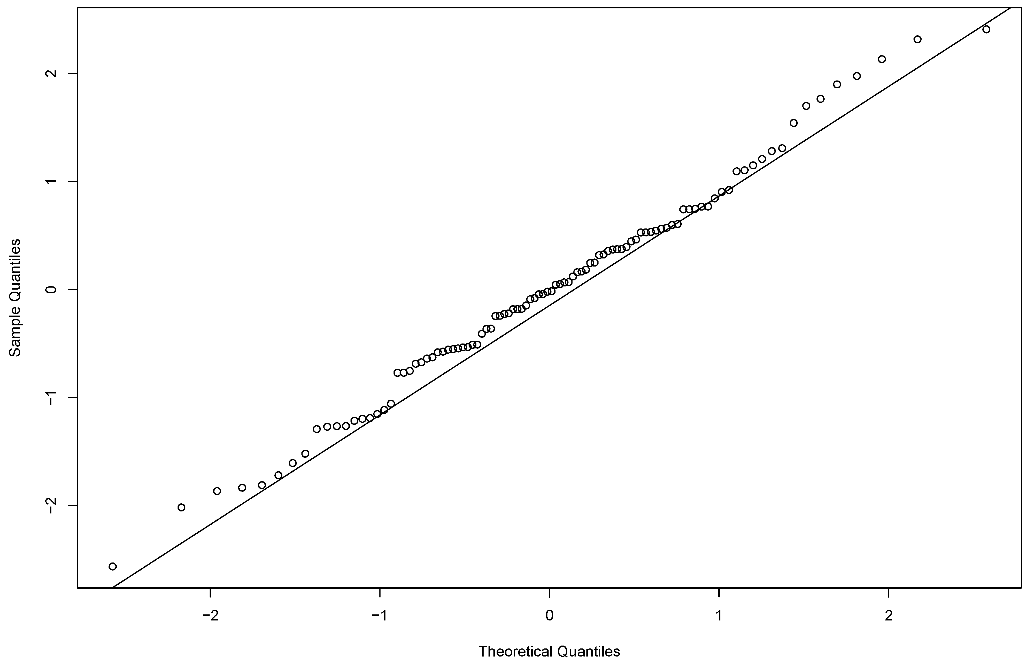
4.1. Simulation for the Connection between Multivariate Log Gamma and Multivariate Normal Distribution

In this section, we examine the connection between the multivariate log-gamma distribution and the multivariate normal distribution. First, we draw the quantile-quantile (QQ)-plot in Figure 1 to show the normality of q generated from MLG ( 0 , α 1 / 2 V , α 1 , 1 / α 1 ) , when α = 10 , 000 . In addition, we use the Kolmogorov–Smirnov test to examine the connection for one dimensional data. We use a multivariate two-sample test [23] for multivariate dimensional data. We generated one data set of size 100 from the multivariate log-gamma distribution and another data set of size 100 from the multivariate normal distribution and then calculated the p-value from the multivariate two-sample test for comparing these two data sets. Then, we repeated this process 1000 times. We found that 992 out of these 1000 p-values were larger than the significance level of 0.05. That is, in 992 of 1000 times, we did not reject the null hypothesis that the two samples were drawn from the same distribution.

4.2. Simulation for Estimation Performance

In this simulation study, our goal was to examine the estimation performance of the hierarchical model. We set β = ( 1 , 1 , 1 ) . We estimated the parameters in this simulation and report the bias ( bias = 1 m j = 1 m ( β i ( j ) β i ) ), the standard error (SE) ( SE = 1 m j = 1 m ( β i ( j ) β ¯ i ) 2 1 / 2 , where β ¯ i = 1 m j = 1 m β i ( j ) ), and the mean square error (MSE) ( MSE = 1 m j = 1 m ( β i ( j ) β i ) 2 ) in Table 1, where β i is the true value of β i .
We try to predict the parameters close to true mean value of our target random variable and the variance is how scattered for our predictions. From Table 1, using the MLG prior for β , we got a reasonable estimation result because it achieves low bias and low variance simultaneously. Besides, we calculated the coverage probability for each variable, it indicates the 94% coverage probability for each parameter.

4.3. Simulation for Model Selection

In this simulation study, our goal was to study the accuracy of our model selection criteria. We have two different simulations in this section. Simulation 1: we set true β = ( 3 , 0 , 0 ) and calculated the difference between the true model and other candidate models for both criteria. In Figure 2, a difference beyond zero means that the true model had smaller DIC than the candidate model and the difference below zero means that the true model had higher LPML than the candidate model in Figure 2. The true model had the smallest DIC and the largest LPML in 99 of 100 simulated data sets. Simulation 2: we set true β = ( 1 , 0 , 0 ) and the results are shown in Figure 3. In each simulation, we have seven candidate models and one of them is true model and denote the true model as model 5. In Figure 2 and Figure 3, the y-axis is the difference between “candidate model i” with true model. The true model had the smallest DIC in 81 of 100 simulated data sets and the largest LPML in 80 out of 100 simulated data sets. For each replicate dataset, we fit our model with 5000 Markov chain Monte Carlo iterations and treated the first 2000 iterations as burn-in. From Figure 2 and Figure 3, in both simulation studies, we find that DIC and LPML yielded relatively consistent model selection results.

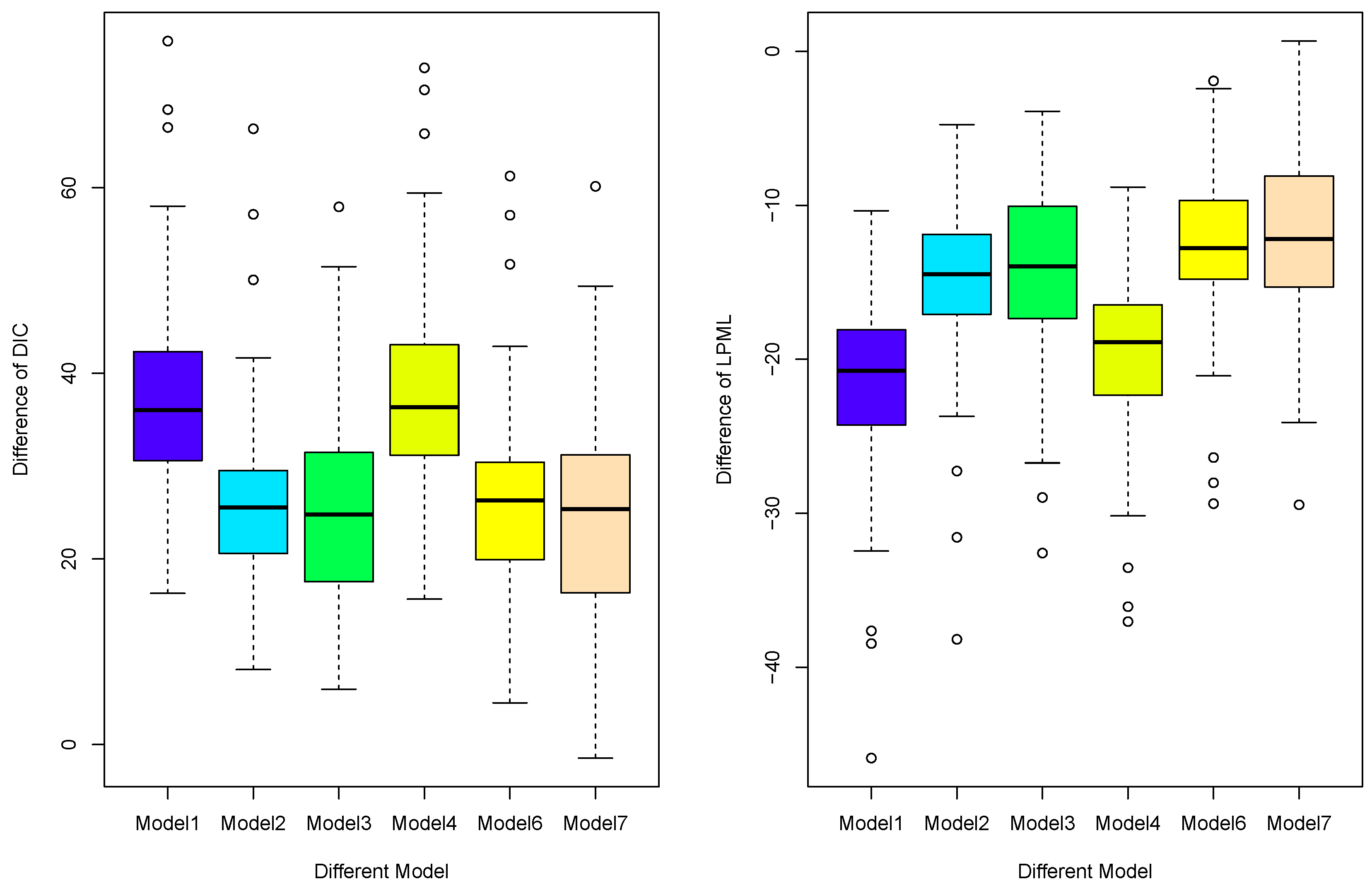
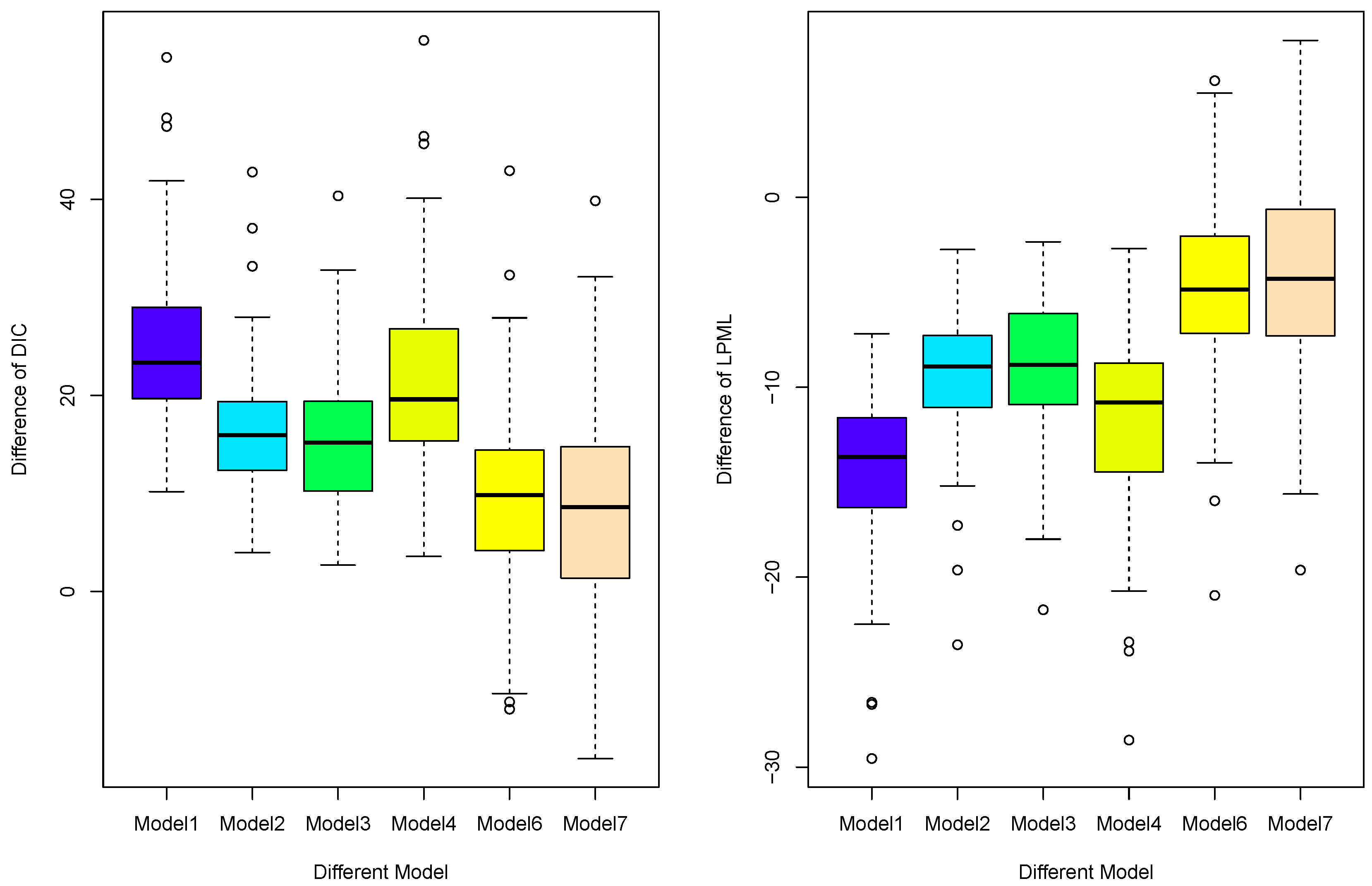
4.4. Simulation for Model Comparison

In this simulation study, our goal is to evaluate the accuracy of our model selection criteria for different spatial random effects model. In this section, we generate the spatial random effects from MLG, W MLG ( 0 n , Σ W 1 / 2 , α W 1 n , κ W 1 n ) , where α W = κ W = 1 . Other settings are same with previous simulations. We generated 100 data sets in these settings. Then, we compared the model fitness based on two following priors:
Prior 1 : W | ϕ , σ w MLG ( 0 n , Σ W 1 / 2 , α W 1 n , κ W 1 n ) , Prior 2 : W | ϕ , σ w N ( 0 n , Σ W ) .
For each replicate dataset, we fit our model with 5000 Markov chain Monte Carlo iterations and treat first 2000 iterations as burn-in. Then, we calculated the difference of DICs and the difference of LPMLs between these two priors. In Figure 4, the values below zero in the left plot imply that prior 1 has smaller DIC than prior 2. Also, the values above zero in the right plot in Figure 4 indicate that prior 1 has higher LPML than prior 2. The results shown in Figure 4 that we have a better result when we use the MLG prior than the Gaussian prior.

5. A Real Data Example

5.1. Data Description

We analyzed seven days of US earthquake data collected in 2018, which includes n = 228 earthquakes that have magnitudes over Z m = 2.44 (https://earthquake.usgs.gov/). We present the earthquake data in Figure 5. We find the data most lie in seismic belts. In Figure 6 and Figure 7, we present the histogram of this data and the scatter plot of this data set. In this analysis we have three variables (depth, gap, rms). The depth is where the earthquake begins to rupture. The gap is the largest azimuthal gap between azimuthally adjacent stations (in degrees). RMS is the root-mean-square (RMS) travel time residual, in sec, using all weights.

5.2. Analysis

We consider the model in Equation (7) and specify α β = 10 5 and κ β = 10 5 . These choices lead to an MLG that approximates a multivariate normal distribution. This choice of hyper-parameters will give an approximately normal prior on β . Inverse gamma priors are chosen for variance parameters σ w 2 and σ 2 , which is a usual choice of the variance parameters in Bayesian analysis. The full conditionals in the Appendix A are used to run a Gibbs sampler. We have seven candidate models in total, and β = ( β 1 , β 2 , β 3 ) = (depth, gap, rms). The number of iterations of the Gibbs sampler is 15,000, and the number of burn-in iterations is 10,000. The trace plots of posterior samples are provided in the Appendix B to show the convergence of MCMC chain. We also compare to a model when W approximates to Normal. The “DIC N ” and “LPML N ” denote the DIC and LPML for a model when W approximates to normal respectively. Furthermore, we calculated the log probability density (LPD) for candidate models. Based on the results in Table 2, the three criteria selected the same model with β 1 and MLG spatial random effects. Our proposed criteria had consistent results with the LPD.
From Table 2, we know that the model with β = ( β 1 , 0 , 0 ) has the smallest DIC and largest LPML. We also report the posterior estimates under the best model in Table 3 according to both DIC and LPML.
From these posterior estimates, the model we select just contains depth as the important covariates and 95% credible interval does not contain zero. We see that as the depth increases, the expected value of earthquakes magnitudes increases. The other two covariates, gap and RMS, have no significant effects on earthquake magnitudes. In other words, from these seven-day earthquake data, deep earthquakes will have bigger magnitudes than shallow earthquakes. From the posterior estimates of ϕ and σ w 2 , we can find that there exists spatial correlation of earthquake magnitudes between different locations. In addition, using MLG as spatial random effects increases the goodness of fit of regression model in this data. This result is consistent with the earthquake literature [2].

6. Discussion

In this paper, we propose a Bayesian variable selection criterion for a Bayesian spatial-temporal model for analyzing earthquake magnitudes. Our main methodological contributions are to use the multivariate log-gamma model for both the regression coefficients and spatial random effects and to do variable selection for regression covariates with spatial random effects. Both DIC and LPML have a good selection power to choose the true model. But Bayesian model assessment criteria such as DIC and LPML do not perform well in the high-dimensional case, because the number of candidate models is very large when the number of covariates increases a lot. Developing a high-dimensional variable selection procedure is one of the important future works. The other future work is to fit other earthquake magnitudes models such as the gamma model or the Weibull model. In addition, we need to propose some Bayesian model assessment criterion to select the true data model for earthquake magnitudes. For the nature hazards problem, we need to incorporate the temporal dependent structure of earthquakes. Recently, the ETAS model [24] (combining the Gutenberg–Richter law and the Omori law) has been widely studied. Modelling earthquake dynamics is an important approach for preventing economic loss caused by an earthquake. Incorporating self-exciting effects in our generalized linear model with spatial random effects is another important future work. Furthermore, we only consider earthquake information as the covariates in our model. It will increase the predictive accuracy for us to combine more geographical information such as fault line information or crustal movement in the future.

Author Contributions

Data curation, G.H.; Formal analysis, H.-C.Y.; Investigation, H.-C.Y.; Methodology, G.H.; Project administration, G.H.; Software, H.-C.Y.; Supervision, M.-H.C.; Visualization, H.-C.Y.; Writing—original draft, G.H.; Writing—review & editing, M.-H.C.

Funding

Chen’s research was partially supported by NIH grants #GM70335 and #P01CA142538. Hu’s research was supported by Dean’s office of College of Liberal Arts and Sciences in University of Connecticut.

Conflicts of Interest

The authors declare no conflict of interest.

Appendix A. Full Conditionals Distributions for Pareto Data with Latent Multivariate Log-Gamma Process Models

From the hierarchical model in Equation (7), the full conditional distribution for β satisfies:
f ( β | · ) f ( β ) f ( Z | · ) exp i ( X ( s i ) β + W ( s i ) ) i ( log ( Z ( s i ) log ( Z m ) ) exp ( X ( s i ) β + W ( s i ) ) × exp α β 1 p Σ β 1 / 2 β κ β 1 p exp ( Σ β 1 / 2 β ) .
Rearranging terms we have
f ( β | · ) exp α β H β β κ β exp ( H β β ) ,
which implies that f ( β | · ) is equal to cMLG ( H β , α β , κ β ) , which is a shorthand for the conditional MLG distribution used in [20].
Similarly, the full conditional distribution for W satisfies:
f ( W | · ) f ( W ) f ( Z | · ) exp i ( X ( s i ) β + W ( s i ) ) i ( log ( Z ( s i ) log ( Z m ) ) exp ( X ( s i ) β + W ( s i ) ) × exp α W 1 n Σ W 1 / 2 W κ W 1 n exp ( Σ W 1 / 2 W ) .
Rearranging terms we have
f ( W | · ) exp α W H W W κ W exp ( H W W ) ,
which implies that f ( W | · ) is equal to cMLG ( H W , α W , κ W ) . Thus we obtain the following full-conditional distributions to be used within a Gibbs sampler:
β cMLG ( H β , α β , κ β ) W cMLG ( H W , α W , κ W ) σ 2 MLG ( 0 , Σ β 1 / 2 , α β 1 p , κ β 1 p ) × IG ( a 1 , b 1 ) σ w 2 MLG ( 0 , Σ W 1 / 2 , α w 1 n , κ w 1 n ) × IG ( a 2 , b 2 ) ϕ MLG ( 0 n , Σ W 1 / 2 , α w 1 n , κ w 1 n ) × IG ( a 3 , b 3 ) ,
where “cMLG” is the conditional multivariate log gamma distribution from [20]. A motivating feature of this conjugate structure is that it is relatively straightforward to simulate from a cMLG. For σ 2 , σ w 2 and ϕ , we consider using a Metropolis–Hasting algorithm or slice sampling procedure [25].
The parameters of the conditional multivariate log gamma distribution are organized into in Table A1.
Table A1. Parameters of the full conditional distribution.
ParameterForm
H β X Σ β 1 / 2
α β 1 n × 1 α β 1 p × 1
κ β ( 1 ) ( log ( Z ( s ) ) log ( Z m ) ) 1 n e W 1 κ β 1 p
H W I n Σ W 1 / 2
α W 1 n × 1 α W 1 n × 1
κ W ( 1 ) ( log ( Z ( s ) ) log ( Z m ) ) 1 n ( e X β ) 1 κ W 1 n

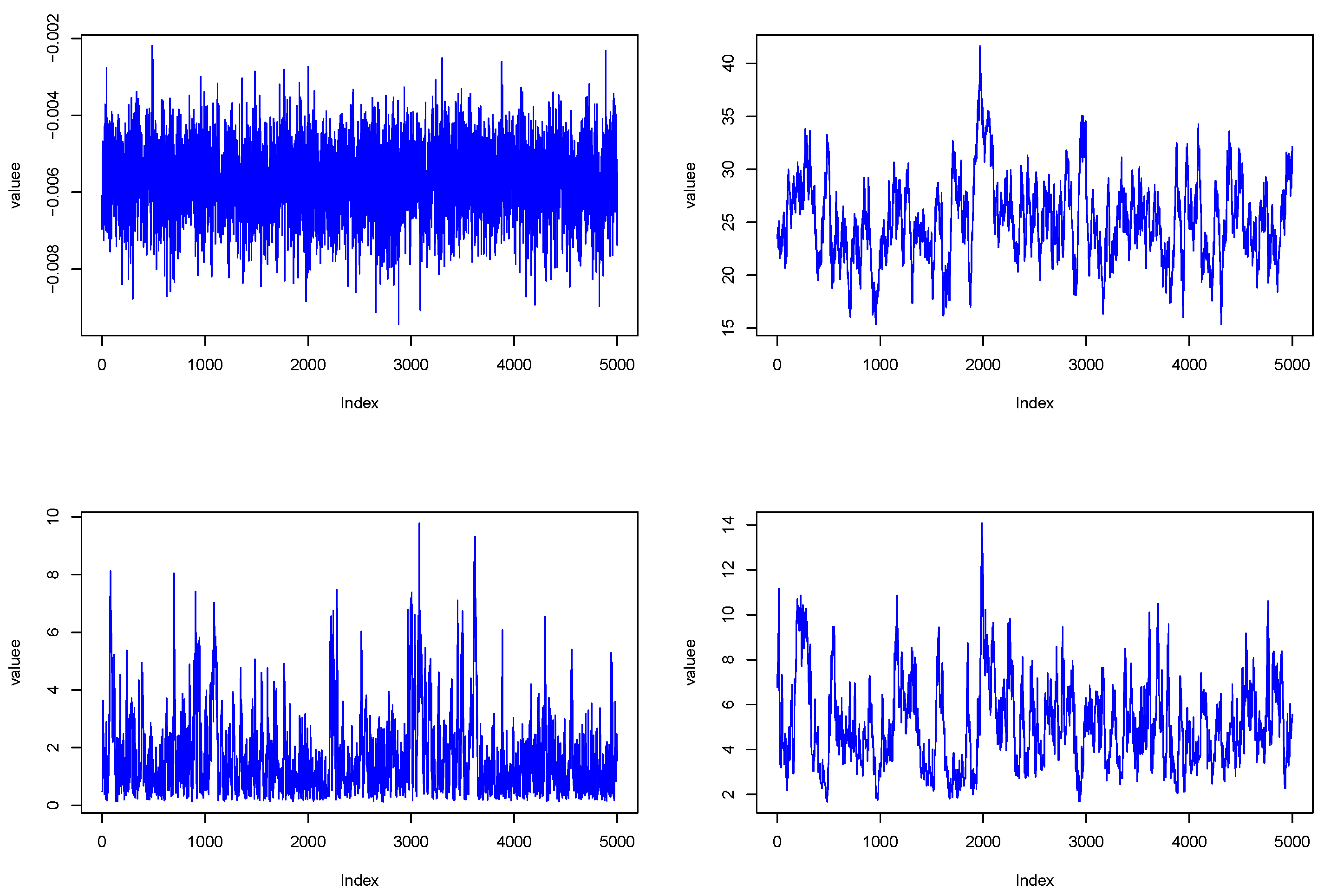
Appendix B. Trace Plot in Real Data Analysis

Figure A1. (upper left) Trace plot for β ; (upper right) Trace plot for ϕ ; (lower left) Trace plot for σ 2 ; (lower right) Trace plot for σ w 2 .
Geosciences 09 00169 g0a1

References

  1. Mega, M.S.; Allegrini, P.; Grigolini, P.; Latora, V.; Palatella, L.; Rapisarda, A.; Vinciguerra, S. Power-law time distribution of large earthquakes. Phys. Rev. Lett. 2003, 90, 188501. [Google Scholar] [CrossRef] [PubMed]
  2. Kijko, A. Estimation of the maximum earthquake magnitude, m max. Pure Appl. Geophys. 2004, 161, 1655–1681. [Google Scholar] [CrossRef]
  3. Vere-Jones, D.; Robinson, R.; Yang, W. Remarks on the accelerated moment release model: Problems of model formulation, simulation and estimation. Geophys. J. Int. 2001, 144, 517–531. [Google Scholar] [CrossRef]
  4. Charpentier, A.; Durand, M. Modeling earthquake dynamics. J. Seismol. 2015, 19, 721–739. [Google Scholar] [CrossRef] [Green Version]
  5. Hu, G.; Bradley, J. A Bayesian spatial—Temporal model with latent multivariate log-gamma random effects with application to earthquake magnitudes. Stat 2018, 7, e179. [Google Scholar] [CrossRef]
  6. Johnson, J.B.; Omland, K.S. Model selection in ecology and evolution. Trends Ecol. Evol. 2004, 19, 101–108. [Google Scholar] [CrossRef] [PubMed] [Green Version]
  7. Cressie, N.; Calder, C.A.; Clark, J.S.; Hoef, J.M.V.; Wikle, C.K. Accounting for uncertainty in ecological analysis: The strengths and limitations of hierarchical statistical modeling. Ecol. Appl. 2009, 19, 553–570. [Google Scholar] [CrossRef] [PubMed]
  8. Akaike, H. Information theory and an extension of the maximum likelihood principle. In Selected Papers of Hirotugu Akaike; Springer: Berlin, Germany, 1973; pp. 199–213. [Google Scholar]
  9. Schwarz, G. Estimating the dimension of a model. Ann. Stat. 1978, 6, 461–464. [Google Scholar] [CrossRef]
  10. Gelfand, A.E.; Dey, D.K. Bayesian model choice: Asymptotics and exact calculations. J. R. Stat. Soc. Ser. B (Methodol.) 1994, 56, 501–514. [Google Scholar] [CrossRef]
  11. Geisser, S. Predictive Inference; Routledge: Abingdon, UK, 1993. [Google Scholar]
  12. Ibrahim, J.G.; Laud, P.W. A predictive approach to the analysis of designed experiments. J. Am. Stat. Assoc. 1994, 89, 309–319. [Google Scholar] [CrossRef]
  13. Spiegelhalter, D.J.; Best, N.G.; Carlin, B.P.; Van Der Linde, A. Bayesian measures of model complexity and fit. J. R. Stat. Soc. Ser. B Stat. Methodol. 2002, 64, 583–639. [Google Scholar] [CrossRef] [Green Version]
  14. Chen, M.H.; Huang, L.; Ibrahim, J.G.; Kim, S. Bayesian variable selection and computation for generalized linear models with conjugate priors. Bayesian Anal. 2008, 3, 585. [Google Scholar] [CrossRef] [PubMed]
  15. Bradley, J.R.; Holan, S.H.; Wikle, C.K. Bayesian Hierarchical Models with Conjugate Full-Conditional Distributions for Dependent Data from the Natural Exponential Family. arXiv, 2017; arXiv:1701.07506. [Google Scholar]
  16. Chen, M.H.; Ibrahim, J.G. Conjugate priors for generalized linear models. Stat. Sin. 2003, 13, 461–476. [Google Scholar]
  17. Geisser, S.; Eddy, W.F. A predictive approach to model selection. J. Am. Stat. Assoc. 1979, 74, 153–160. [Google Scholar] [CrossRef]
  18. Tobler, W.R. A computer movie simulating urban growth in the Detroit region. Econ. Geogr. 1970, 46, 234–240. [Google Scholar] [CrossRef]
  19. Gelfand, A.E.; Schliep, E.M. Spatial statistics and Gaussian processes: A beautiful marriage. Spat. Stat. 2016, 18, 86–104. [Google Scholar] [CrossRef]
  20. Bradley, J.R.; Holan, S.H.; Wikle, C.K. Computationally Efficient Distribution Theory for Bayesian Inference of High-Dimensional Dependent Count-Valued Data. arXiv, 2015; arXiv:1512.07273. [Google Scholar]
  21. Chen, M.H.; Shao, Q.M.; Ibrahim, J.G. Monte Carlo Methods in Bayesian Computation; Springer Science and Business Media: Berlin/Heidelberg, Germany, 2012. [Google Scholar]
  22. Liang, H.; Wu, H.; Zou, G. A note on conditional AIC for linear mixed-effects models. Biometrika 2008, 95, 773–778. [Google Scholar] [CrossRef] [PubMed]
  23. Baringhaus, L.; Franz, C. On a new multivariate two-sample test. J. Multivar. Anal. 2004, 88, 190–206. [Google Scholar] [CrossRef]
  24. Ogata, Y. Statistical models for earthquake occurrences and residual analysis for point processes. J. Am. Stat. Assoc. 1988, 83, 9–27. [Google Scholar] [CrossRef]
  25. Neal, R.M. Slice sampling. Ann. Stat. 2003, 31, 705–741. [Google Scholar] [CrossRef]
Figure 1. QQ-plot.
Figure 1. QQ-plot.
Geosciences 09 00169 g001
Figure 2. Deviance information criterion (DIC) and logarithm pseudo marginal likelihood (LPML) difference between candidate models and true model (model 5) of Simulation 1 ((left) DIC, (right) LPML).
Geosciences 09 00169 g002
Figure 3. DIC and LPML difference between candidate models and true model (model 5) of Simulation 2 ((left) DIC, (right) LPML).
Geosciences 09 00169 g003
Figure 4. DIC and LPML difference ((left) DIC, (right) LPML).
Geosciences 09 00169 g004
Figure 5. Map of US earthquake data.
Geosciences 09 00169 g005
Figure 6. Histogram of US earthquake data collected in 2018.
Geosciences 09 00169 g006
Figure 7. Scatter plot of earthquakes magnitudes, depth, gap and root-mean-square (RMS).
Geosciences 09 00169 g007
Table 1. Estimation performance.
ParameterTrue ValueBiasSEMSECoverage Probability
β 1 1−0.02720.29030.0850.94
β 2 1−0.00240.29390.08630.94
β 3 1−0.01020.33690.11350.94
Table 2. Deviance information criterion (DIC) logarithm pseudo marginal likelihood (LPML), and log probability density (LPD) of candidate models.
ModelDICLPMLLPDDIC N LPML N LPD N
β 1 , β 2 , β 3 3058.71−1535.68−1528.583325.47−1669.44−1661.86
β 1 , β 2 2936.72−1472.54−1469.383130.42−1569.94−1564.33
β 1 , β 3 3037.96−1522.69−1516.973258.84−1633.79−1628.54
β 2 , β 3 3056.02−1533.71−1526.383322.33−1666.84−1660.28
β 1 2890.80−1446.60−1445.7892958.61−1480.68−1478.42
β 2 2908.10−1457.28−1452.353073.28−1540.16−1535.76
β 3 3034.67−1519.84−1518.623896.29−1951.31−1947.27
Table 3. Posterior estimation under the best model.
Posterior MeanStandard Error95% Credible Interval
β 1 −0.005680.0009616(−0.00763, −0.00389)
ϕ 24.86934.5693(17.5827, 35.1427)
σ 2 2.16202.4563(0.2642, 9.1086)
σ w 2 4.93041.7632(2.1670, 8.8958)

