Meta-Analysis of Satellite Observations for United Nations Sustainable Development Goals: Exploring the Potential of Machine Learning for Water Quality Monitoring

Abstract

This review paper adopts bibliometric and meta-analysis approaches to explore the application of supervised machine learning regression models in satellite-based water quality monitoring. The consistent pattern observed across peer-reviewed research papers shows an increasing interest in the use of satellites as an innovative approach for monitoring water quality, a critical step towards addressing the challenges posed by rising anthropogenic water pollution. Traditional methods of monitoring water quality have limitations, but satellite sensors provide a potential solution to that by lowering costs and expanding temporal and spatial coverage. However, conventional statistical methods are limited when faced with the formidable challenge of conducting pattern recognition analysis for satellite geospatial big data because they are characterized by high volume and complexity. As a compelling alternative, the application of machine and deep learning techniques has emerged as an indispensable tool, with the remarkable capability to discern intricate patterns in the data that might otherwise remain elusive to traditional statistics. The study employed a targeted search strategy, utilizing specific criteria and the titles of 332 peer-reviewed journal articles indexed in Scopus, resulting in the inclusion of 165 articles for the meta-analysis. Our comprehensive bibliometric analysis provides insights into the trends, research productivity, and impact of satellite-based water quality monitoring. It highlights key journals and publishers in this domain while examining the relationship between the first author’s presentation, publication year, citation count, and journal impact factor. The major review findings highlight the widespread use of satellite sensors in water quality monitoring including the MultiSpectral Instrument (MSI), Ocean and Land Color Instrument (OLCI), Operational Land Imager (OLI), Moderate Resolution Imaging Spectroradiometer (MODIS), Thematic Mapper (TM), Enhanced Thematic Mapper Plus (ETM+), and the practice of multi-sensor data fusion. Deep neural networks are identified as popular and high-performing algorithms, with significant competition from extreme gradient boosting (XGBoost), even though XGBoost is relatively newer in the field of machine learning. Chlorophyll-a and water clarity indicators receive special attention, and geo-location had a relationship with optical water classes. This paper contributes significantly by providing extensive examples and in-depth discussions of papers with code, as well as highlighting the critical cyber infrastructure used in this research. Advances in high-performance computing, large-scale data processing capabilities, and the availability of open-source software are facilitating the growing prominence of machine and deep learning applications in geospatial artificial intelligence for water quality monitoring, and this is positively contributing towards monitoring water pollution.

1. Introduction

Water pollution is a growing global concern due to its adverse effects on the economy, safety, the environment, and human health [1]. Despite this problem, there is a lack of proper monitoring, and as a result, there are insufficient water quality monitoring data to show the extent of pollution [2]. Traditional sampling and laboratory methods used for water quality monitoring are constrained by several limitations. These limitations include high costs, time-consuming procedures, exposure to safety risks during sampling and laboratory analysis, and low spatial and temporal resolution [3,4,5,6]. As a result, these constraints lead to inadequate and insufficient water quality monitoring data. However, satellite data can effectively bridge this gap by offering a cost-effective and convenient method that yields real-time results [7]. This enables the timely and accurate identification of water quality problems, facilitating the monitoring of water quality [8]. Thus, satellite data has the potential to revolutionize the way water quality monitoring is conducted, providing a more comprehensive understanding of water pollution at a planetary scale [9].

The growth of satellite remote sensing has led to a significant increase in the production of geospatial big data. This expansion of capabilities in global environmental monitoring from space is made possible by the in-depth historical archives and long-time series satellite data that is now available [10]. This has resulted in opportunities for users to understand how anthropogenic pressures, land use and land cover changes (LULCCs), climate change, industrial and agricultural productivity, global population growth, and rapid urbanization have affected water quality. The rapid production and availability of geospatial data have led to a significant surge in its volume, velocity, and variety, commonly referred to as the 3Vs [11]. This surge presents challenges in archiving, storing, analyzing, and interpreting the data. To tackle these challenges, cluster-based high-performance computing (HPC) systems and cloud platforms have emerged as popular solutions [12]. As the volume, variety, and velocity of geospatial data continue to grow, cluster-based HPC systems provide powerful computing capabilities by utilizing a network of interconnected computers.

These systems enable the parallel processing of large-scale geospatial data, allowing for efficient data analysis and interpretation. With their ability to distribute computational tasks across multiple nodes, cluster-based HPC systems can significantly enhance the speed and scalability of geospatial data processing [12]. Cloud platforms, on the other hand, provide a flexible and scalable infrastructure for managing geospatial data. Cloud platforms enable the seamless storage, retrieval, and analysis of large volumes of geospatial data by leveraging the resources of remote servers. Cloud services’ on-demand nature allows researchers to adapt their computational resources based on fluctuating data demands, resulting in cost-efficiency and scalability. Both cluster-based HPC systems and cloud platforms contribute to mitigating the 3Vs of geospatial data challenges. They enable researchers, scientists, and data analysts to leverage advanced computing capabilities and scalable infrastructure for efficient and effective geospatial data management. They provide new opportunities to derive valuable insights from satellite data by leveraging visualization techniques and trend analyses, enhancing their application in the field of water quality monitoring.

These valuable satellite-derived insights can be applied to a variety of environmental issues affecting water quality, including climate change and variability, ecosystem degradation, LULCCs, and natural resource management. In the field of data-driven satellite-based water quality monitoring, various AI techniques, including time-series forecasting, classification, regression predictions, computer vision, and natural language processing (NLP), play pivotal roles. These techniques predict and forecast emergency critical events such as algal blooms, ensuring the safety and sustainability of our water resources. The application of these insights has the potential to significantly improve water resources management, sustainability, and resilience.

2. Scope and Objectives of the Review

This section will outline the previous reviews on the topic and describe the contributions of this study. The scope and objectives of the review, including the research questions and inclusion or exclusion criteria, will also be presented. Previous reviews of the remote sensing literature have been marked by a proclivity towards a broad and generalized overview of the field, owing to their focus on multiple types of remote sensing approaches or on expansive fields of specialization that encompass diverse areas such as forestry, water, agriculture, urban planning, environmental monitoring, disaster management, defense, wildlife, and many more. Additionally, these reviews have been found to lack comprehensive bibliometric analyses or meta-analyses, which could potentially offer an in-depth understanding of the existing body of literature.

Ogashawara [13] analyzed trends in Phycocyanin detection using bibliometric analysis, while Khan et al. [14] applied a meta-analysis approach to give an overview of spatiotemporal trends in HAB determination using remote sensing techniques on a planetary scale. Holloway and Mengersen [15] broadly reviewed statistical machine learning applications for the attainment of United Nations World Bank Sustainable Development Goals, including water quality. Gholizadeh et al. [16] evaluated the use of sensors on board various remote sensing platforms to monitor eleven water quality parameters (WQPs). Wang and Yang [17] tracked progress made in the monitoring and evaluation of WQPs using remote sensing methods but focused only on China inland lakes. Hassan and Woo [18] reviewed machine learning applications in water quality using satellite data but did not review the performance used in method evaluation for ML, and their review did not include bibliometric analysis to show research trends.

Mukonza and Chiang [19] conducted another review highlighting the potential of machine and deep learning classifiers, based on high-resolution optical sensors and synthetic-aperture radar (SAR) satellites, for monitoring micro- and macroplastics in aquatic ecosystems. Specifically, SAR satellites can detect changes in backscatter signal, which is a function of surface roughness in water bodies, primarily caused by wind-driven waves. Microplastics present on the ocean surface can also impact surface roughness, leading to a weaker radar backscatter signal. High-resolution optical sensors can also be used to detect microplastics in water by measuring spectral reflectance. Reviews previously conducted on the subject of satellite-based water quality monitoring using machine and deep learning have identified several gaps. These gaps include a lack of specific focus on the use of AI for water quality monitoring, as well as the absence of a critical analysis that quantifies the performance, application, and effectiveness of satellites, AI algorithms, geolocation, and WQPs.

A multitude of studies exploring the potential of leveraging machine and deep learning to monitor water quality through satellite observations have in some cases produced divergent and conflicting results. These studies have reported inconsistent and contrasting model performance across a range of water quality parameters, satellite sensors, and algorithms, ultimately leading to divergent and contradictory findings. As a result, significant evidence gaps exist in the application of machine and deep learning techniques to satellite-based water quality monitoring. The current review uses a rigorous approach that combines both bibliometric and meta-analysis to systematically evaluate and synthesize previous research in order to address this evidence gap. The review’s specific goal is to derive conclusions regarding the different factors affecting and influencing the performance of regression algorithms in predicting water quality using satellite data.

These factors include the form of satellite sensor used, the particular AI technique applied, the water quality parameter being investigated, and the geographic location of the study area. Despite the fact that image preprocessing methods such as geometric correction (GC), atmospheric correction (AC), and radiometric correction (RC) methods may have an impact on how accurately satellite images turn to estimate water quality, this review does not include them because of the inconsistent ways in which they have been reported in the literature. As a result, there are not sufficient points of information to conduct a thorough analysis in this regard. Instead, a lot of researchers have made use of easily accessible items like analysis ready data (ARD), which does not require a lot of preprocessing.

Our study, in contrast to the highlighted reviews, focuses on streamlining specific tasks related to machine and deep learning for satellite-based water quality monitoring. The primary objective of our research is to highlight the challenges associated with water quality while demonstrating how machine learning can improve the accuracy, certainty, and reliability of estimation using regression prediction tasks. This review aims to provide a focused and thorough analysis of the use of satellite sensors in monitoring water quality using machine and deep learning, with a particular focus on water pollution research. The following are the objectives of this review:

• To provide up-to-date insights into the latest trends and advancements in the application of artificial intelligence for water quality monitoring using satellite remote sensing.
• To provide a comprehensive overview of the topic of satellite remote sensing and its specific applications in monitoring water quality with machine and deep learning.
• To evaluate the strengths and limitations of various satellite sensors and machine/deep learning techniques used for water quality monitoring.
• To identify gaps in the existing body of remote sensing water quality literature and suggest future research directions.

The following research questions will guide this review:

• What are the current trends and advancements in the use of satellite remote sensing and AI for water quality monitoring, and what implications do they have for the field?
• What are the different types of satellite sensors used for water quality monitoring, and how have they been utilized in various domains?
• What are the different types of machine learning algorithms used in water quality monitoring, and how have they been applied?
• What are the strengths and limitations of various sensors and machine/deep learning techniques in solving specific research questions related to water quality monitoring?
• What are the gaps in the existing remote sensing literature on water quality monitoring, and what future research directions can be suggested to address these gaps?

The paper is structured into a comprehensive framework of eleven cohesive sections, each playing a crucial role in unraveling the complexities of machine and deep learning applications in satellite-based water quality observations. Commencing with Section 1, the introduction of the domain research area, laying the groundwork for understanding the profound impact of these advanced techniques on water quality monitoring. Section 2 proceeds to explain the research landscape, navigating through related works that have been published prior to this research to pinpoint existing gaps and limitations, setting the stage for our innovative contributions. In Section 3, the methods applied in this study come to the fore, meticulously synthesizing, collecting, presenting, visualizing, and rigorously analyzing the data underpinning our investigation. The ensuing Section 4, Section 5 and Section 6—embody the heart of our findings, with Section 4 presenting bibliometric results, while Section 5 and Section 6 deftly summarize the intricate machine and deep learning algorithms and satellite sensors deployed, respectively.Section 7 undertakes a sweeping exploration of global water resources status in light of pollution and water quality, unearthing the transformative role played by satellite sensors in monitoring pollution levels in these vital resources. Section 8 also makes an important contribution by further enhancing our insights through a comprehensive meta-analysis, scrutinizing model performance across various domains, including how our choices of machine or deep learning models, satellite sensors, water quality parameters, water classes, and geo-locations of water bodies can affect the accuracy of our results, methodically analyzing 165 studies to extract meaningful and contextualized results.

Section 9 and Section 10 list the hardware and software cyber infrastructure requirements in this research domain, disclosing essential online resources and programming languages that play pivotal roles in executing these complex tasks. Notably, our research takes a pioneering step, providing publicly available code for free, empowering the wider community with the tools to advance their own investigations. In Section 11, we address the inherent limitations and research gaps, outlining valuable recommendations and the prospects for future studies. Lastly, our major findings are summarized in the conclusion.

3. Methods

We aim to investigate the extent to which machine and deep learning applications have been utilized and performed in satellite-based water quality monitoring. While previous studies have suggested that these artificial intelligence techniques are gaining traction in this field, few have conducted a quantitative assessment of their usage. Therefore, we conducted a comprehensive search of the Scopus indexed database from 2005 to the present, using the query string: (TITLE-ABS-KEY (Water quality) AND TITLE-ABS-KEY (“Satellite sensors”) OR TITLE-ABS-KEY (“Machine learning/Deep learning”) OR TITLE-ABS-KEY (neural networks, support vector machines, linear regression, random forest, boosted trees, Gaussian process regression) OR TITLE-ABS-KEY (artificial intelligence) OR TITLE-ABS-KEY (water pollution)) AND PUBYEAR > 2004 AND (LIMIT-TO (DOCTYPE, “ar”)). The Preferred Reporting Items for Systematic Reviews and Meta-analyses (PRISMA) 2020 [20] flow diagram for new systematic reviews, shown in Figure 1, was used to review literature for satellite-based water quality monitoring in the following steps: define research questions, study selection, data extraction, data synthesis, and reporting.

4. Bibliometric Results

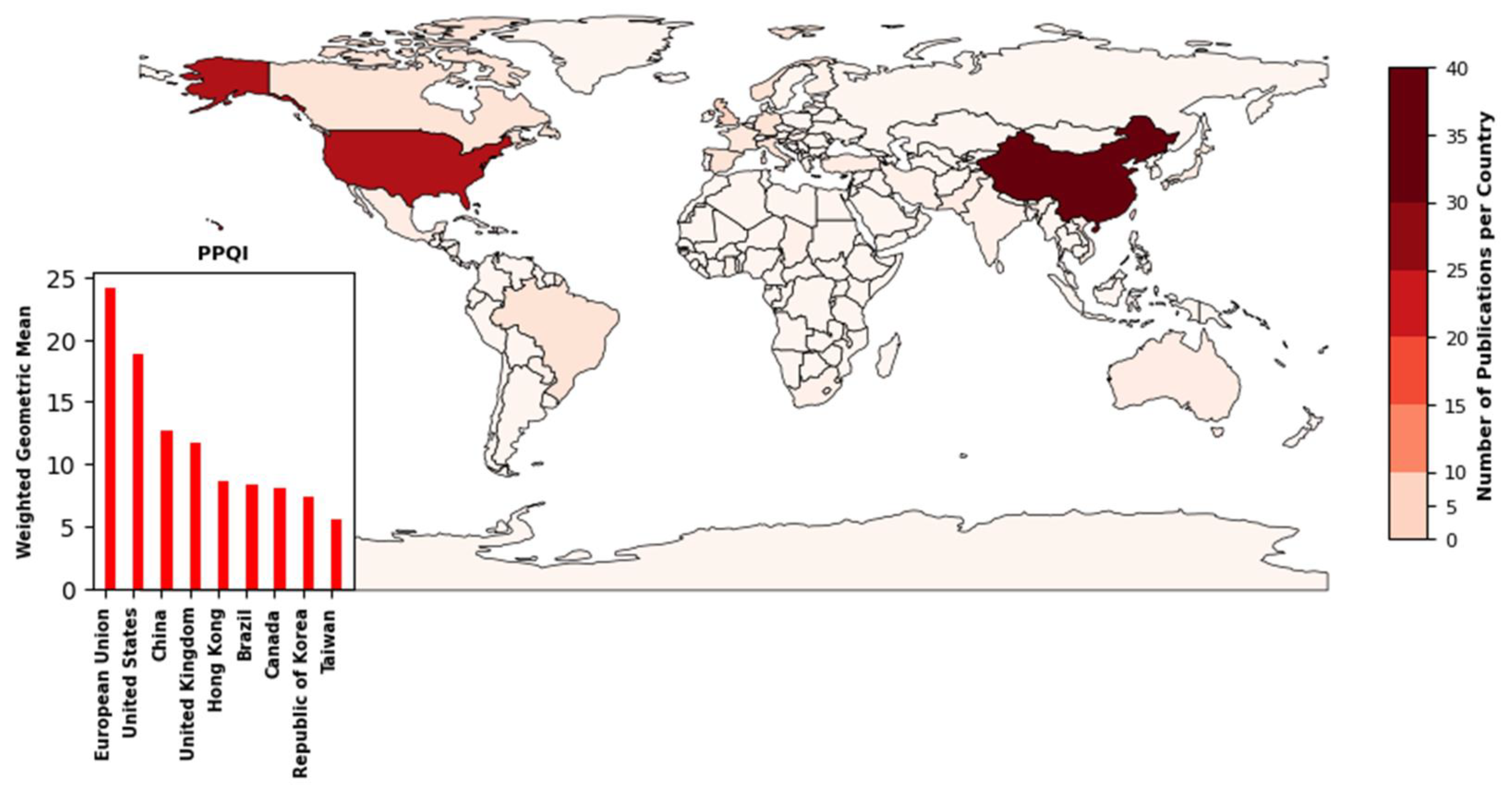
4.1. Author Affiliation, Country and Productivity

After reviewing all the relevant literature used in the meta-analysis, it was found that 35 publications (21.2%) on machine and deep learning for satellite-based water quality monitoring were authored by researchers from China, with 32 (19.4%) and 30 (18.2%) publications by researchers from the United States of America (U.S) and the European Union (EU) excluding the United Kingdom (UK), respectively (refer to Figure 2). These regions have made significant investments in research and development of satellites, machine and deep learning, and artificial intelligence technologies resulting in the development of specialized expertise and resources in these areas. This could be a possible explanation as to why researchers from the U.S. and China have emerged as dominant players in this field. Additionally, the presence of well-established space agencies and satellite manufacturing companies in these countries could also provide an advantage to researchers in this area.

Our bibliometric analysis looked at the number of machine and deep learning satellite-based water quality monitoring articles published in the 165 high-quality Scopus index journals tracked by an index we developed based on a weighted geometric mean called the publication production quality index (PPQI), which takes into account total number of publications per country, the impact factor of journals where papers where published, and the number of citations the papers received, to measure the quality of the AI papers. The data used for computing these indices were based on the journal metrics of the selected 165 articles for the meta-analysis. The PPQI was crafted through a methodical process that assigned specific relevance weights to key metrics: the number of citations (weighted as high relevance = 3), impact factor (moderate relevance = 2), and the number of publications (minimum relevance = 1). These relevance weights were normalized to maintain proportionality, resulting in a balanced evaluation. Firstly, the geometric mean for each factor is determined by taking the nth root of the product of the factor raised to its corresponding geometric weight, where n is the total number of considered factors. Subsequently, the weighted geometric mean is calculated by combining the normalized weights and the geometric means of each factor.

$$PPQI=\sqrt{{GM}_{NC}^{1/2}\times {GM}_{IF}^{1/3}\times {GM}_{NP}^{1/6}}$$

(1)

where ${GM}_{NC},{GM}_{IF},and{GM}_{NP}$ represents the geometric mean of number of citations, geometric mean of impact factor, and geometric mean of number of publications, respectively.

The EU combined (excluding the United Kingdom) outperformed the U.S, China, the UK, and Hong Kong in that descending order. China, having increased its output in journals over recent years, leads in terms of productivity. Although it is third in terms of both productivity and quality, publication numbers are not the whole story, and papers from China were cited about 20% less than the world average for the whole period considered, whereas papers from the US were cited about 40% more than average (see Figure 2). Producing a large quantity of papers without ensuring their lasting impact may not be the most effective approach.

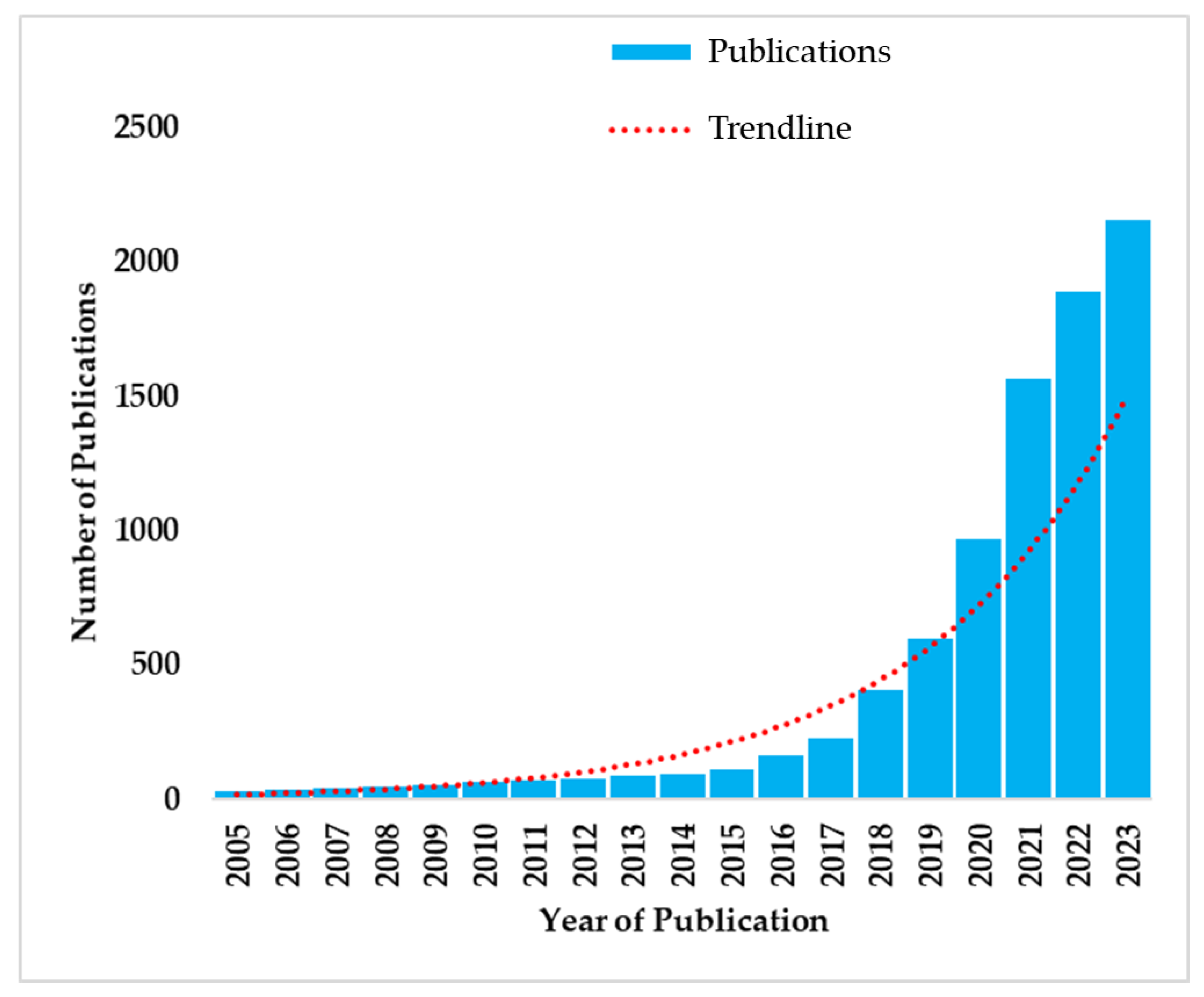
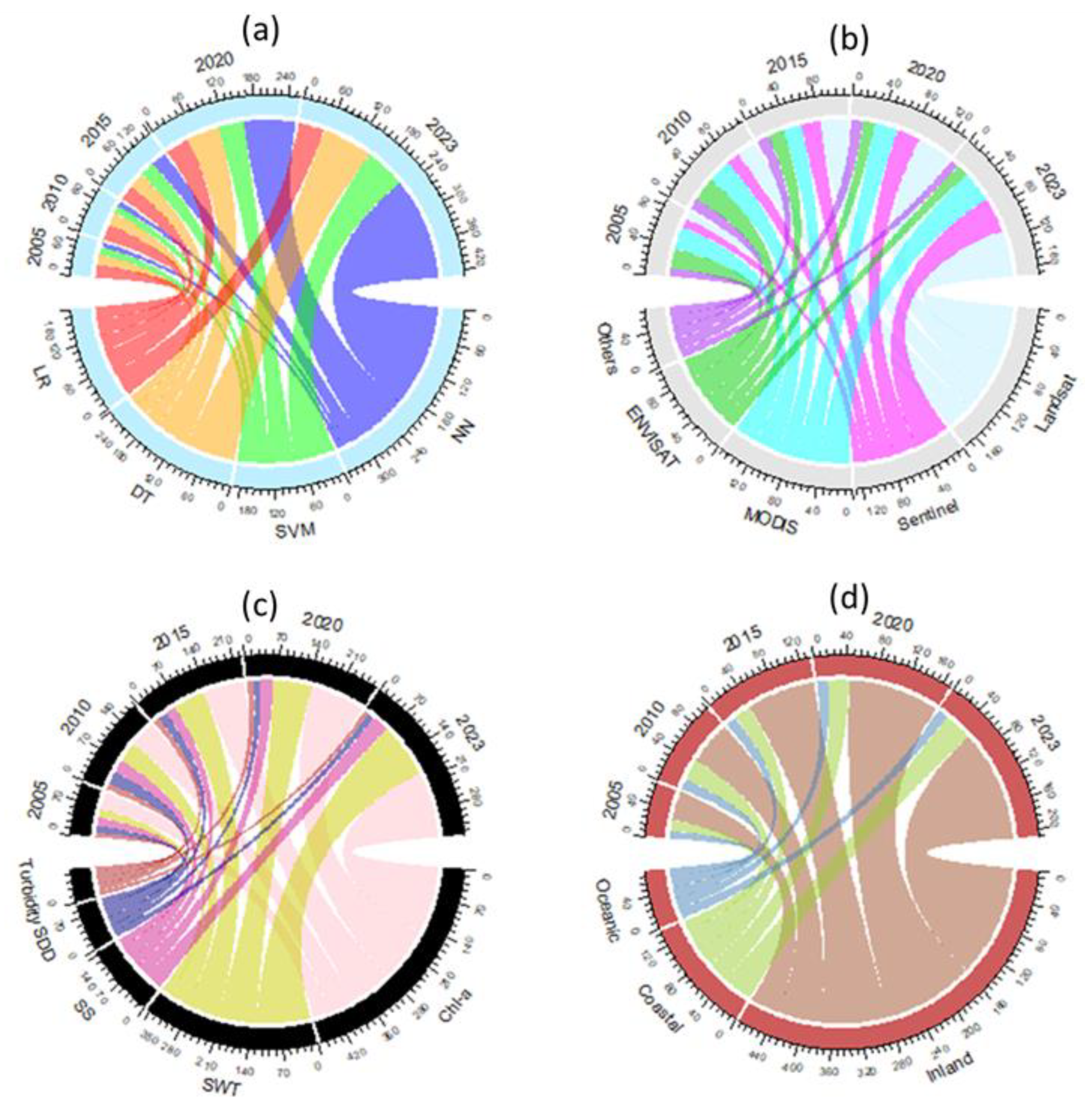
4.2. Research Trends

Through analyzing the frequency and trends of publications in this domain, we provide an understanding of the growth and potential impact of machine and deep learning techniques in water quality monitoring using satellite observations. Overall, we identified an increasing number of publications over time for all search criteria (Figure 3).

Notably, the number of publications related to machine and deep learning methodologies has grown rapidly in comparison to those related to satellite technology (Figure 4a,b). However, both trends are slightly lower than the trend for the specific water quality search (Figure 4c). This indicates that machine learning techniques, particularly neural networks (NNs), random forests (RFs), and support vector machine (SVM), have become increasingly popular in recent years, likely due to their accuracy and ability to handle complex data. On the other hand, traditional methods, like principal component analysis (PCA) and linear regression (LR), are being used less frequently. Neural networks, are experiencing faster growth than satellite technology. Satellite-based water quality investigations coupled with artificial intelligence have gained significant attention in inland ecosystems applications, followed by estuaries and coastal ecosystems. Surprisingly, oceanic water ecosystems, despite having a significant role in regulating climate change, have been the least explored in this regard (see Figure 4d). Our findings thus highlight the importance of understanding and utilizing machine learning techniques for water quality researchers in order to stay appraised of the latest developments in the field because the day-to-day human responsibilities in water quality monitoring are evolving.

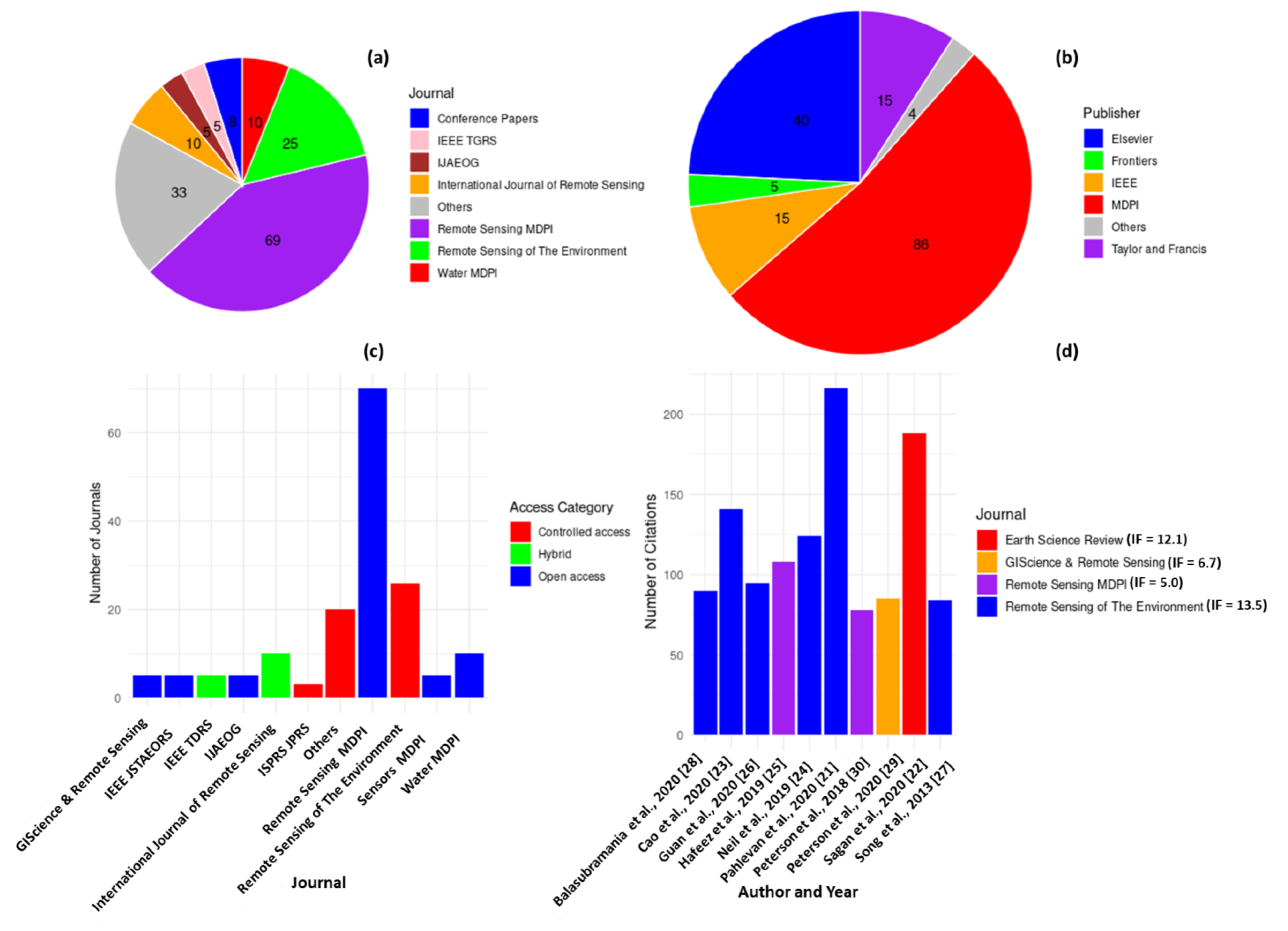
4.3. Influential Papers, Journals, and Publishers

We performed a bibliometric analysis on a curated selection of papers within the domain of satellite observations for water quality monitoring. The objective was to assess the research output and impact of this field, while also identifying emerging research trends.

Notably, our results emphasize the prominence of the journals Remote Sensing (42%) and Remote Sensing of the Environment (15%), and the International Journal of Remote Sensing and MDPI Water tied at 6% (Figure 5a). The publisher MDPI was associated with the majority of publications (52.1%), followed by Elsevier (24%), and Taylor and Francis and IEEE are tied at 12.1%, also having a significant presence (Figure 5b). This analysis categorized research paper journals into open access, controlled access, and a hybrid approach, visually represented by a bar chart. While open access journals contained more articles, this did not significantly impact the number of citations for these papers. MDPI dominates open access journals, making up over half of the total considered journal papers. In contrast, controlled access, primarily represented by Elsevier, comprises roughly one-third of the studied journals. This discrepancy is attributed to cost considerations; open access often involves article processing charges (APCs), while controlled access may require subscription fees or paywalls for readers. (Figure 5c). Elsevier journals with high publication activity included Remote Sensing of the Environment, International Journal of Applied Earth Observation and Geoscience (IJAEOG), and ISPRS Journal of Photogrammetry and Remote Sensing (ISPRS JPRS). Furthermore, the study successfully identified the top ten most cited papers in this research area, with citation counts ranging from 78 to 216 [21,22,23,24,25,26,27,28,29,30] (Figure 5d). Notably, the paper by Pahlevan et al. [21] received the most citations, totaling 216. Sagan et al. [22], Cao et al. [23], Neil et al. [24], and Hafeez et al. [25] were close behind. The top ten cited papers in the field of remote sensing for water quality research that received significant attention had impact factors ranging from 5 to 13.5 [21,22,23,24,25,26,27,28,29,30] (Figure 5d). This range underscores the significant influence these papers have on the scholarly community and solidifies their importance within the domain.

5. An Overview of Machine and Deep Learning Techniques Used in Satellite-Based Water Quality Monitoring

Table 1. Summary of machine and deep learning techniques used in satellite-based water quality monitoring.

Learning Method	Task Application Type	Algorithm Type	Algorithm Name	Reference
Supervised	Regression	Linear	OLS	Ansari et al. [31]
			RR	Tenjo et al. [35]
			LASSO	Silveira Kupssinskü et al. [34]
			EN	Acar-Denizli et al. [37]
			PLSR	Sagan et al. [22]
		Polynomial	Cubic	Ruescas et al. [33]
		SVM	Linear	Zhang et al. [44]
			Gaussian Radial Basis Function (RBF) kernel	Zhang et al. [45]
			Polynomial	Ruescas et al. [33]
		BTs	Adaptive Boosting (AdaBoost)	Leggesse et al. [47]
			Gradient Boosting Models (GBM)	Leggesse et al. [47]
			eXtreme Gradient Boosting (XGBoost)	Cao et al. [23]
			Light Gradient-Boosting Machine (LightGBM)	Su et al. [48]
			Categorical Data Gradient Boosting (CatBoost)	Chen et al. [3]
		DTs	Classification and Regression Trees (CARTs)	Xu et al. [49]
		Ensemble Trees	RFs	Du et al. [39]
		Neural networks	Multilayer Perceptron (MLP)	Martinez et al. [40]
			RNN	Qi et al. [41]
			Long Short-Term Memory (LSTM)	Kim et al. [42]
			CNN	Syariz et al. [43]
			Data INterpolating Convolutional Auto-Encoder (DINCAE)	Jung et al. [50]
		Lazy learner	k-Nearest Neighbor (k-NN)	Qiao et al. [51]
Unsupervised	Dimensionality Reduction	Feature extraction	PCA	Kong et al. [52]
			Data INterpolating Empirical Orthogonal Function (DINEOF)	Guo et al. [53]

is an organized taxonomy providing an overview of commonly used machine and deep learning techniques in satellite-based water quality monitoring. The table is organized with techniques classified according to their learning type and further subcategorized according to their application type and specific algorithm names. Different machine and deep learning regressors have been used in satellite-based water quality monitoring. Table 1 provides an overview of these algorithms, which include ordinary least square (OLS)-based methods and their variants, such as simple linear regression [31], multiple linear regression (MLR) [32], polynomial regression [33], least absolute shrinkage and selection operator regression (LASSO) or L1 [34], ridge regression (RR) or L2 [35], Bayesian ridge regression (BRR) [36], and elastic net (EL) or L1&2 [37]. There are also tree-based algorithms such as decision trees (DTs) [38], boosted trees (BTs) [23], and ensemble trees, like RFs [39], included. Neural networks (NNs) or artificial neural networks (ANNs) as they are commonly known [40], which include feed-forward neural networks (FFNN) [30], recurrent neural networks (RNN) [22,41,42], and convolutional neural networks (CNN) [43], have emerged as the go-to algorithms in this field. In this domain, SVMs have also proven to be highly adaptable, with researchers experimenting through selecting different kernel functions that best suit their data, such as sigmoid, linear, radial basis function (RBF), or polynomial [44]. Researchers have paid less attention to gene programming (GP) [45], Gaussian process regression (GPR) [46], and partial least-squares regression (PLSR) algorithms [47].

6. An Overview of Satellite Ocean Color Sensor Design Concepts and Performance Requirements

Table 2 provides an overview of the identified 20 satellite sensors that have been utilized in satellite-based water quality monitoring. The specific examples of sensor categorization as listed in Table 2 is outlined as follows: whisk-broom scanning spectroradiometers include Landsat 5 Multispectral Scanner (MSS), Landsat 7 Enhanced Thematic Mapper Plus (ETM+), Geostationary Ocean Color Imager II (GOCI-II), and HuanJing (HJ)—Charge-Coupled Device (CCD). Push-broom imaging spectrometers are represented by Wide Field View Multispectral Camera (GF-6 WFV), Environmental Mapping and Analysis Program (EnMAP), Sea-viewing Wide Field-of-view Sensor (SeaWiFS), Sentinel-3 Ocean and Land Color Instrument (OLCI), Landsat 8 Operational Land Imager (OLI), Sentinel-2 MultiSpectral Instrument (MSI), and WorldView-2 and -3 (WV-2 and -3). Typical linear variable filter imaging spectrometers include the Airborne Visible/Infrared Imaging Spectrometer (AVIRIS). Staring image radiometers are exemplified by Landsat 8 Thermal Infrared Sensor (TIRS), Visible Infrared Imaging Radiometer Suite (VIIRS), and Moderate Resolution Imaging Spectroradiometer (MODIS). Imaging radar is represented by Sentinel-1 Synthetic-Aperture Radar (SAR). Image Fourier transform spectrometers are showcased by EO-1 Hyperion.

The summary emphasizes that the predominant imaging system designs used for water quality monitoring are push-broom spectroradiometry imaging, followed closely by whisk-broom scanning spectroradiometry and staring imaging spectrometry. In contrast, Linear Variable Filter Imaging Spectrometer, Imaging Fourier Transform Spectrometer, and imaging radar sensor satellites have been employed to a much lesser extent, with only one instance of use reported for each. The different types of satellite sensors used in water quality monitoring have their unique advantages and disadvantages. Push-broom scanning spectroradiometers have been widely used due to their long dwell time over each ground resolution cell, which increases the signal strength and results in high radiometric resolution [54,55,56,57]. However, these sensors have low spatial resolution. Additionally, the data collected by push-broom sensors may contain cross-track camera discontinuities.

Whisk-broom scanning spectroradiometry and staring imaging spectrometry are also commonly used sensor designs for water quality monitoring. These sensors are capable of covering a wider swath width compared to push-broom sensors, allowing them to cover a larger area of the Earth’s surface in a single pass. However, the along-track striping artifacts are common in these sensors, which can result in reduced image quality. The Linear Variable Filter Imaging Spectrometer and Imaging Fourier Transform Spectrometer are two other sensor designs that have been used to a lesser extent. These sensors use different mechanisms to separate incoming light into its spectral components, resulting in high spectral resolution [54,55,56,57]. However, the spatial resolution of these sensors is typically lower compared to push-broom and whisk-broom sensors [54,55,56,57]. Finally, imaging radar sensor satellites are another alternative for water quality monitoring. These sensors use microwave frequencies to penetrate through the water surface and retrieve information about subsurface features such as water depth and bottom type. However, these sensors have limited spatial resolution and may not be suitable for certain applications where high-resolution imagery is required [58]. The selection of the appropriate sensor design for water quality monitoring depends on the specific application and the trade-offs between spectral, spatial, and radiometric resolutions. Table 2 specifically categorizes the different sensors applied to water quality into their imaging systems, stating their advantages and disadvantages.

Table 2. Overview of Satellite Sensor Imaging Systems and Their Applications in Water Quality Monitoring.

Sensor Name	Type of Imaging System	Advantages	Disadvantages	Applications in Water Quality	References
MSS	Whisk-broom Scanning Spectroradiometer	Provides relatively high resolution in terms of both spatial and spectral domains, and a wider swath width compared to push-broom sensors, allowing them to cover a larger area of the Earth’s surface in a single pass	Limited to only four spectral bands and a single detector resulting in low spatial resolution	Used for mapping water resources and monitoring water quality	[59]
AVIRIS	Linear Variable Filter Imaging Spectrometer	High spectral resolution (up to 224 bands)	Slow scanning speed and high data storage requirements	Used for mapping water resources, water quality monitoring, and bathymetry	[60]
Hyperion	Imaging Fourier Transform Spectrometer	High spectral resolution (up to 242 bands)	Relatively small coverage area and low spatial resolution	Used for mapping water resources and water quality monitoring	[61]
SeaWiFS	Push-broom Imaging Spectrometer	High radiometric resolution and low noise	Limited spectral range and low spatial resolution	Used for monitoring ocean color and primary productivity	[62]
OLCI	Push-broom Imaging Spectrometer	Longer dwell time over each ground resolution cell increases the signal strength (high radiometric resolution, no pixel distortion)	Varying sensitivity for detectors	Applied in ocean color	[63]
ETM+	Whisk-broom Scanning Spectroradiometer	Improved signal-to-noise ratio and spatial resolution compared to previous Landsat sensors	Limited to only seven spectral bands	Used for monitoring water resources and detecting water quality changes	[64]
OLI	Push-broom Imaging Spectrometer	Higher signal-to-noise ratio and improved spatial resolution compared to previous Landsat sensors	Limited to only nine spectral bands	Used for monitoring water resources and detecting water quality changes	[65,66]
TIRS	Staring Imaging Radiometer	Measures thermal radiation, provides temperature data	No visible light data, lower spatial resolution	Used for monitoring surface water temperature	[67]
MSI	Push-broom Imaging Spectrometer	High spatial resolution (up to 10 m)	Limited to only 13 spectral bands	Used for monitoring water resources and detecting water quality changes	[68]
MODIS) Aqua & Terra	Staring Imaging Spectrometer	Large spatial coverage with global coverage in 1–2 days	Relatively low spatial resolution and limited spectral range	Used for monitoring water temperature, ocean color, and aquatic vegetation	[18]
HJ—CCD	Whisk-broom Scanning Spectroradiometer	High spatial resolution (up to 2.5 m)	Limited spectral range and lower radiometric resolution	Used for monitoring water resources and detecting water quality changes	[69]
SAR	Imaging Radar	All-weather and day-and-night imaging capability	Limited to only detecting surface features and roughness	Used for monitoring water resources and detecting water quality changes	[70]
VIIRS	Staring Imaging Spectrometer	High spatial resolution and spectral range	Limited to only 22 spectral bands	Used for monitoring water temperature, ocean color, and aquatic vegetation	[71]
GOCI-II	Whisk-broom Scanning Spectroradiometer	High temporal resolution and large coverage area	Limited to only eight spectral bands	Used for monitoring water quality and marine ecosystem health	[72]
EnMAP	Push-broom Imaging Spectrometer	High spectral resolution and accurate calibration	Limited spatial coverage and spectral range	Used for monitoring water quality, aquatic vegetation, and bathymetry	[73]
GF-6 WFV	Push-broom Imaging Spectrometer	High spatial resolution and spectral range	Limited to only four spectral bands	Used for monitoring water quality, aquatic vegetation, and bathymetry	[74]
WV 2	Push-broom Imaging Spectrometer	High spatial resolution and spectral range	Limited to only eight spectral bands	Used for monitoring water quality and aquatic vegetation	[75]
WV 3	Push-broom Imaging Spectrometer	High spatial resolution and spectral range	Limited to only eight spectral bands	Used for monitoring water quality and aquatic vegetation	[76]

Table 2. Overview of Satellite Sensor Imaging Systems and Their Applications in Water Quality Monitoring.

Sensor Name	Type of Imaging System	Advantages	Disadvantages	Applications in Water Quality	References
MSS	Whisk-broom Scanning Spectroradiometer	Provides relatively high resolution in terms of both spatial and spectral domains, and a wider swath width compared to push-broom sensors, allowing them to cover a larger area of the Earth’s surface in a single pass	Limited to only four spectral bands and a single detector resulting in low spatial resolution	Used for mapping water resources and monitoring water quality	[59]
AVIRIS	Linear Variable Filter Imaging Spectrometer	High spectral resolution (up to 224 bands)	Slow scanning speed and high data storage requirements	Used for mapping water resources, water quality monitoring, and bathymetry	[60]
Hyperion	Imaging Fourier Transform Spectrometer	High spectral resolution (up to 242 bands)	Relatively small coverage area and low spatial resolution	Used for mapping water resources and water quality monitoring	[61]
SeaWiFS	Push-broom Imaging Spectrometer	High radiometric resolution and low noise	Limited spectral range and low spatial resolution	Used for monitoring ocean color and primary productivity	[62]
OLCI	Push-broom Imaging Spectrometer	Longer dwell time over each ground resolution cell increases the signal strength (high radiometric resolution, no pixel distortion)	Varying sensitivity for detectors	Applied in ocean color	[63]
ETM+	Whisk-broom Scanning Spectroradiometer	Improved signal-to-noise ratio and spatial resolution compared to previous Landsat sensors	Limited to only seven spectral bands	Used for monitoring water resources and detecting water quality changes	[64]
OLI	Push-broom Imaging Spectrometer	Higher signal-to-noise ratio and improved spatial resolution compared to previous Landsat sensors	Limited to only nine spectral bands	Used for monitoring water resources and detecting water quality changes	[65,66]
TIRS	Staring Imaging Radiometer	Measures thermal radiation, provides temperature data	No visible light data, lower spatial resolution	Used for monitoring surface water temperature	[67]
MSI	Push-broom Imaging Spectrometer	High spatial resolution (up to 10 m)	Limited to only 13 spectral bands	Used for monitoring water resources and detecting water quality changes	[68]
MODIS) Aqua & Terra	Staring Imaging Spectrometer	Large spatial coverage with global coverage in 1–2 days	Relatively low spatial resolution and limited spectral range	Used for monitoring water temperature, ocean color, and aquatic vegetation	[18]
HJ—CCD	Whisk-broom Scanning Spectroradiometer	High spatial resolution (up to 2.5 m)	Limited spectral range and lower radiometric resolution	Used for monitoring water resources and detecting water quality changes	[69]
SAR	Imaging Radar	All-weather and day-and-night imaging capability	Limited to only detecting surface features and roughness	Used for monitoring water resources and detecting water quality changes	[70]
VIIRS	Staring Imaging Spectrometer	High spatial resolution and spectral range	Limited to only 22 spectral bands	Used for monitoring water temperature, ocean color, and aquatic vegetation	[71]
GOCI-II	Whisk-broom Scanning Spectroradiometer	High temporal resolution and large coverage area	Limited to only eight spectral bands	Used for monitoring water quality and marine ecosystem health	[72]
EnMAP	Push-broom Imaging Spectrometer	High spectral resolution and accurate calibration	Limited spatial coverage and spectral range	Used for monitoring water quality, aquatic vegetation, and bathymetry	[73]
GF-6 WFV	Push-broom Imaging Spectrometer	High spatial resolution and spectral range	Limited to only four spectral bands	Used for monitoring water quality, aquatic vegetation, and bathymetry	[74]
WV 2	Push-broom Imaging Spectrometer	High spatial resolution and spectral range	Limited to only eight spectral bands	Used for monitoring water quality and aquatic vegetation	[75]
WV 3	Push-broom Imaging Spectrometer	High spatial resolution and spectral range	Limited to only eight spectral bands	Used for monitoring water quality and aquatic vegetation	[76]

7. Satellite Applications for Water Resources and Quality Monitoring

Water covers approximately two-thirds of the Earth’s surface, amounting to a total volume of 332.5 million cubic miles [77,78,79,80]. Unfortunately, 97.5% of the world’s water resources are saline, with 96.5% being oceanic water and the remaining 1% being saline inland water resources [77,78,79,80]. This leaves only 2.5% global freshwater resources available, and out of this freshwater, over 68% is frozen in ice and glaciers, while the remaining 30% is stored as groundwater [77,78,79,80]. Despite their scarcity, groundwater and surface freshwater sources such as wells, aquifers, springs, rivers, and lakes are the primary sources of water for human consumption [77,78,79,80]. However, they only account for about 22,300 cubic miles of water, and this translates to approximately 0.7% of the total water resources. Freshwater ecosystems serve as the primary sources of water for various essential purposes, such as drinking, hydro-power generation, industrial water supply, support for biodiversity, recreation, water transportation, waste management, irrigation, and aquaculture [77,78,79,80]. In addition, freshwater aquatic ecosystems play a crucial role in supporting human development activities; however, these same activities have a negative impact on the same water resources. Climate change, industrialization, urbanization, population dynamics, agricultural development, and changes in land use and land cover have all contributed to environmental changes in aquatic systems [80,81,82,83,84,85,86,87,88]. An estimated 80% of municipal and industrial wastewater is being discharged into freshwater ecosystems annually without prior treatment, recycling, or reuse [89]. These changes result in nutrient pollution, drought, extreme events, and contamination, all of which adversely affect aquatic ecosystems. The negative effects include the proliferation of toxic blue-green algae, extreme turbidity, ocean heat waves, warming water bodies, and accelerated eutrophication, which significantly impact the sustainability of water resources.

Pollution of water resources is a complex and ubiquitous environmental issue that can have severe and often interconnected impacts on aquatic ecosystems. Eutrophication [90], acidification [91], sedimentation [92], toxic chemicals [93,94], microplastics [95,96], and thermal pollution [97] are some of the most serious manifestations of this problem. Eutrophication is a condition that occurs when excessive nitrogen and phosphorus nutrient loads enter a water body, leading to a series of acute symptoms with two primary symptoms of eutrophication which are hypoxia (or oxygen depletion) and the proliferation of harmful algal blooms, which can severely affect aquatic ecosystems through destroying aquatic life in affected areas [98]. Irrigation and rain-fed induced surface run-off, the application of fertilizer, grazing, indiscriminate discharge of untreated sewage from wastewater treatment plants, and economic growth around watersheds, particularly in industrial areas, are contributory factors towards eutrophication [99].

The rapid expansion of urban areas in many watersheds is transforming the natural landscape and replacing wetlands, forests, and grasslands with impermeable pavements that reduce the infiltration rate of rainwater into the ground [100,101]. This phenomenon causes an increase in the volume and speed of stormwater runoff, which leads to decreased groundwater recharge, erosion of sediment, and an overall decline in water quality [102]. The growing urban population exacerbates these challenges by placing increasing pressure on wastewater treatment infrastructure. The volume of sewage and other pollutants produced by human activity can quickly surpass the capacity of existing wastewater treatment facilities, leading to overflow and runoff into freshwater sources [102]. Climate-change-induced extreme rainfall events, such as floods, compound these issues by further overwhelming wastewater treatment infrastructure and causing an increase in wastewater treatment plant (WWTP) runoff and overflow [103]. The negative impact of urbanization on water resources manifests in several ways, including increased flooding, sediment erosion, and stormwater overflow. These challenges have a significant effect on water quality degradation and can also impact the availability of water resources for human and ecological use. In addition to its negative impact on water quality, eutrophication is recognized as a significant contributor to greenhouse gas emissions, which have far-reaching effects on the global environment [104].

Water acidification is a form of pollution that occurs when water pH decreases due to elevated atmospheric CO₂ levels and organic matter respiration. The relationship between eutrophication-induced algal blooms and water pH is complex; while some blooms can temporarily increase pH through photosynthesis, the overall impact varies based on factors like bloom size, duration, and respiratory processes during decay. Acidification is mainly due to CO₂ reaction with water, forming carbonic acid and releasing hydrogen ions (H⁺) and bicarbonate ions (${HCO}_3^{-}$). Sulfur dioxide and nitrogen oxide uptake can also create acidic compounds, like carbonic, nitrous, and sulfuric acids, further affecting pH. These pH fluctuations harm aquatic life, especially pH-sensitive species like fish, amphibians, and invertebrates, and can trigger the release of toxic metal contaminants from sediment, which are harmful to aquatic ecosystems [105].

Sedimentation is a form of water pollution caused by the introduction of organic and inorganic matter, including soil particles, into rivers, lakes, and streams as suspended or settleable solids in the water column [106]. Excessive sedimentation can reduce water clarity and increase turbidity, decreasing light penetration and dissolved oxygen levels and harming aquatic organisms [106,107]. In addition to reducing clarity, increasing turbidity, and decreasing dissolved oxygen levels, sedimentation can also contribute to the transport of various pollutants [92,106,107,108,109]. For example, sediment-laden pollutants such as agrochemicals, including herbicides, pesticides, and fertilizer nutrients, as well as microplastics, can be carried into water bodies by sedimentation [92,106,107,108,109]. These pollutants transported by sedimentation contribute towards eutrophication, toxic chemical pollution, and microplastic pollution in water. Sediment transport into water is not only influenced by natural processes, such as rainfall run-off and ice-melt, but also by human activities that increase soil erosion, such as land use changes, construction activities, and deforestation. Climate-change-induced extreme rainfall events, landslides, or glacial melts can exacerbate the issue by increasing sediment-laden pollutants based soil erosion into aquatic ecosystems [106,107,108,109]. These events can cause more soil erosion and transport, leading to higher sedimentation rates in water bodies. Furthermore, sedimentation can change the physical structure of an ecosystem, affecting aquatic organism habitats and altering the food chain. Human activities such as mining and dredging can also contribute to sedimentation. In addition to reducing water quality, sedimentation can also have economic impacts by reducing the capacity of water storage reservoirs and hydropower plants [110,111]. It can also increase the risk of flooding by reducing the capacity of rivers and streams to carry water.

Toxic chemical water pollution comes from sources such as industrial activities, agricultural practices, and untreated industrial, human, and animal effluents [112,113]. Heavy metals, pesticides, and pharmaceuticals are among the toxic chemicals that can contaminate water, posing significant health risks to aquatic life and humans who use or come into contact with contaminated water [112,113]. Macro-, meso-, micro-, and nanoplastics, a range of small to large plastic particles, have become a growing concern in recent years [114]. They can enter freshwater ecosystems and harm aquatic organisms as well as accumulate in the food chain, potentially impacting human health. Thermal pollution and warming water bodies are as a result of increase in water temperature caused by human activities [115,116]. These activities can range from the discharge of warm water from power plants, deforestation, urbanization, industrial or power generation processes, and the discharge of heated water into natural water bodies [115,116]. This can harm aquatic life and disrupt the natural balance of the ecosystem. Climate change represents a critical and ongoing stressor that affects the ecological health of water systems. Extensive research has clearly shown that climate change has a negative impact on water quality in a variety of aquatic ecosystems. Nonetheless, isolating the precise effects of climate change from the complex interaction of multivariate factors influencing water quality is a formidable challenge. Water pollution is an urgent global environmental challenge that requires immediate attention. To effectively protect, restore, and manage water resources, it is essential to understand water quality and monitor it regularly.

Water quality is a multidimensional evaluation of the overall state of health, and characteristics of an aquatic ecosystem encompass physical, chemical, biological, thermal and radiological properties [117,118]. WQPs are traditionally classified into physical, chemical, and biological indicators [117,118]. Physical parameters include properties such as pH, water temperature, dissolved oxygen (DO), total suspended solids (TSS), electrical conductivity (EC), salinity or total dissolved solids (TDS), nutrients like nitrogen and phosphorus, and aesthetics (such as odor, color, and taints) [119]. Chemical parameters include cations (e.g., calcium, potassium, and magnesium) and anions (e.g., nitrates, sulfates, and chlorides) [119]. Biological parameters include the presence of microorganisms, like viruses, algae, and bacteria, like Escherichia coli (E. coli) and total coliforms [120]. The traditional system of water quality classification covers all forms of pollution except for toxic chemicals and microplastics pollution [121,122,123].

Traditional methods of water quality monitoring, such as field measurements and laboratory analysis, are commonly used in water quality monitoring. Wet chemical analysis involves the separation of samples based on characteristics such as color, odor, or melting point using techniques such as extraction, precipitation, or distillation [124,125]. The substance’s quantity is then determined by measuring its weight, volume, or color. Modern analytical chemistry, on the other hand, is based on instrumental analysis. Analytical instruments such as atomic and molecular spectrometers, electrochemical analysis instruments, nuclear magnetic resonance, X-rays, and mass spectrometers are available [126]. While traditional methods for monitoring water quality, such as field measurements and laboratory analysis, are widely accepted for their accuracy and reliability, they are often constrained by various factors, including limited spatiotemporal resolution, high costs, and time-consuming and labor-intensive processes [127,128,129,130]. These limitations make it challenging to obtain real-time data and monitor water quality on a large scale. As a result, alternative methods, such as remote sensing and machine learning algorithms, have gained popularity for their ability to overcome these constraints and provide more efficient and effective water quality monitoring solutions [131,132,133,134,135]. These methods can enable the collection and analysis of data from large water bodies, and can provide a more comprehensive understanding of water quality conditions at a higher spatiotemporal resolution, at a lower cost, and with less labor intensity [131,132,133,134,135].

Water quality monitoring is transitioning away from traditional sampling and laboratory methods and advancing towards the use of remote sensing technologies, specifically satellite remote sensing. Since their inception, satellite sensors have undergone significant evolution and improvement, enabling the acquisition of increasingly detailed and precise information for the assessment and management of water quality. The Landsat mission pioneered the observation of the Great Lakes in the 1970s, where data obtained from satellite sensors enabled the identification of various parameters such as particulate contaminants, whiting events, and Chl-a concentration [136,137,138,139,140,141]. The National Aeronautics and Space Administration (NASA)’s launch of the Coastal Zone Color Scanner (CZCS) aboard the Nimbus-7 satellite in 1978 was a significant breakthrough [136,137,138,139,140,141]. The CZCS is designed to collect ocean color data, providing valuable insights into water quality parameters such as chlorophyll-a (Chl-a) concentration, suspended sediment levels (SS), and the presence of harmful algal blooms (HABs) [136,137,138,139,140,141]. Notable advancements in water quality satellite sensor technology include the CZCS in 1978 [136,137,138,139,140,141], Nimbus 7 Coastal Zone Mapping Experiment (CZME) in 1981 [136,137,138,139,140,141], Landsat-4 Thematic Mapper (TM) in 1982 [136,137,138,139,140,141], SeaWiFS in 1984 [136,137,138,139,140,141], and MODIS in 1999 [136,137,138,139,140,141].

Additional noteworthy contributions also came from the launch of European Space Agency I (ERS-1) SAR in 1992 [136,137,138,139,140,141], Landsat 7 ETM+ and Advanced Spaceborne Thermal Emission and Reflection Radiometer (ASTER) in 2002 [136,137,138,139,140], Terra Aqua MODIS in 2002 [136,137,138,139,140,141], Sentinel-1A in 2014 [136,137,138,139,140,141], Sentinel-2A in 2015 [142], Landsat 8 OLI in 2013 [142], Sentinel-2B in 2017 [142], Sentinel-1B SAR in 2016 [143], Sentinel-3A OLCI in 2016 [144], Sentinel-3B OLCI in 2018 [144], and most recently, Landsat-9 OLI-2 in 2021 [66]. Machine and deep learning techniques have contributed remarkably towards research advancements and achievements in the field of satellite-based water quality monitoring. These approaches have extended the monitoring capabilities beyond optically active matter in water, such as Chl-a and suspended solids [22], to include non-optically-active matter, including DO, EC, and nutrients. Furthermore, recent developments have even ventured into monitoring emerging pollutants, such as microplastics [145,146], enabling a broader and more comprehensive assessment of water quality.

The continuous advancements in satellite sensors has generated massive amounts of high-dimensional data, posing challenges for traditional statistical analysis methods. Consequently, the integration of machine and deep learning techniques has emerged as a powerful approach to leverage the potential of satellite data offering distinct advantages in monitoring optically inactive substances within the water column, showcasing its remarkable flexibility. Such interdisciplinary methodologies for water quality monitoring can be advanced, to facilitate better understanding and monitoring of aquatic ecosystems on a global scale. Despite significant advances in machine learning for satellite-based water quality monitoring, several challenges remain in its application. These difficulties include issues such as bias, trust, privacy, interpretability, and accountability. Addressing these concerns is critical to ensuring the dependability and integrity of the models and data used in water quality monitoring. We can improve the effectiveness and acceptance of machine learning approaches in this critical domain by mitigating bias, increasing transparency, protecting privacy, and establishing accountability mechanisms.

8. Factors Influencing Model Performance in Satellite-Based Water Quality Monitoring Using a Meta-Analysis Approach

This section incorporates a meta-analysis combining and analyzing data from multiple independent studies on the same topic to systematically compare model performance from different studies. Our primary objective was to develop a hypothesis regarding the factors that influence model performance, collect reliable data on model performance, and apply appropriate statistical methods for analyzing the data. Through this process, we drew conclusions and interpreted the results within the context of existing knowledge. Furthermore, the hypothesized factors that potentially influence model performance are analyzed in greater detail.

Silveira Kupssinskü et al. [34] compare machine learning algorithms in monitoring Chl-a and SS, highlighting the influence of different algorithms and water quality parameters on model performance. Modiegi et al. [147] confirm the superior performance of the Sentinel-2 MSI sensor compared to Landsat 8 OLI, Advanced Spaceborne Thermal Emission and Reflection Radiometer (ASTER), and Satellite Pour l’Observation de la Terre 6 (SPOT 6) sensors. Knaeps et al. [148] compare algorithms across different water quality classes, revealing performance variations based on water quality class. Nasir et al. [149] investigate classifier performance across water classes, noting suboptimal performance for the stream class. The aforementioned studies collectively validate the hypothesized factors that have the potential to influence predictive models in the assessment of water quality based on satellite data. These factors include the choice of machine or deep learning algorithm used, the specific satellite sensor employed, the water quality parameters (WQPs) being considered for analysis, and the classification of water quality classes under investigation. This literature focuses primarily on model performance comparisons within the context of single studies. The emphasis in these studies is on providing detailed descriptions of the experimental setup, data collection procedures, and specific evaluation metrics used. The findings are then presented and analyzed in light of the study’s research question or objective.

Single studies are limited by small sample sizes, potential biases, low statistical power, a narrow scope, and a lack of replication. Meta-analysis, the combination of data from multiple studies, can overcome these limitations, resulting in increased statistical power, improved generalizability, reduced bias, quantification of effect sizes, and identification of sources of variability. A meta-analysis is a comprehensive and rigorous approach to evidence synthesis that provides a broader understanding of the research topic while overcoming the limitations of individual studies. To accomplish this, we used R² values as a reliable evaluation metric, allowing us to quantify and compare the predictive capabilities of various models across multiple studies. We hoped to provide a comprehensive and robust analysis of the subject matter by leveraging the power of meta-analysis, ensuring the reliability and validity of our findings.

When comparing the accuracy of models applied in different studies to different datasets or time periods, it is often necessary to use accuracy measures that are independent of the scale of the data. This is because different datasets may have different scales, making direct comparison of accuracy measures difficult and irrational. For example, consider two datasets, one with values ranging from 0 to 100, and another with values ranging from 0 to 1000. If we use a measure like root mean squared error (RMSE), which is calculated by taking the square root of the average squared difference between predicted and actual values, we may find that the RMSE is higher for the second dataset, simply because the values are on a larger scale. To overcome this issue, we can use measures like percentage error or coefficient of determination (R-squared), which are not dependent on the scale of the data [150]. Percentage error is calculated by taking the absolute difference between predicted and actual values, dividing by the actual value, and multiplying by 100. One way to address the issue of giving unequal weight to errors across multiple scales is to utilize metrics based on relative errors or scaled to normalize errors an approach recommended by various researchers, such as Subbotin and Shprits [151] and Zhelavskaya et al. [152]. Athanasiu et al. [153] and Welling [154] also propose using metrics that are scaled to normalize errors.

In our study, a comprehensive examination of the literature was conducted, establishing that most researchers in the field of satellite-based water quality regression modeling prefer to use both the coefficient of determination (R²) and the RMSE as the primary metrics for evaluating model performance. These metrics are widely considered to be the gold standard for evaluating models in this domain. However, there are some exceptions to this trend, as seen in studies conducted by Svendsen et al. [155] and Pahlevan et al. [21], where these researchers primarily focused only on the RMSE as the sole metric for model evaluation. In contrast, there are researchers who have also reported using R² alone or in combination with other evaluation metrics to assess model performance. Notable examples include Song et al. [156], Balasubramanian et al. [28], Bertani et al. [157], Chang et al. [158], Chen et al. [159], Fan et al. [160], and Kravitz et al. [161]. These researchers have utilized a variety of metrics, including mean absolute percentage error (MAPE), mean absolute error (MAE), and bias relative error (RE), to evaluate model performance. In cases where data are normally fitted, the R² value typically falls within the range of 0 to 1. However, it is important to acknowledge that poorly fitted data can sometimes yield negative R² values, as demonstrated by Asim et al. [162]. Their study focused on the development of a Case 2 Regional CoastColour (C2RCC)-net model for Chl-a retrieval, utilizing a match-up criterion based on C2RCC in situ Chl-a measurements. The results of this study revealed negative R² values along with relatively high error evaluation metrics such as RMSE, MEA, and bias. The negative R² values indicate that the chosen C2RCC model’s performance is worse than the null hypothesis, which assumes an identity line fit. It is crucial to emphasize that a negative R² value should not be misconstrued as a mathematical impossibility or a result of a computer bug. Instead, it signifies that the chosen model, with its specific constraints, inadequately captures the underlying trend within the data.

R² provides insights into model data variance explanations, but in complex models, a high R² does not always imply high model performance; it could be due to overfitting and inclusion of irrelevant variables. This requires a cautious use and consideration of other metrics for robust model evaluation. Drawing upon our hypothesized factors that influence satellite-based machine and deep learning models for water quality monitoring, we thoroughly examine the impact of these factors on model performance based on the R² metric. We hope to elucidate the intricate relationships between algorithm selection, sensor selection, water quality parameters, and optical water types by closely examining each factor and how these factors potentially affect the predictive abilities of the models.

8.1. Machine or Deep Learning Model Choice

In our study, we conducted a comprehensive comparative analysis of various supervised machine learning techniques to assess their model performance (Figure 6a). The techniques examined include LR [29,30,31,32,33,34,35,36,45,46,51,65,75,163,164,165,166,167,168,169,170,171,172,173,174,175,176,177,178,179,180,181,182,183,184], PLSR [22,27,185,186,187,188,189], GPR [33,35,46,171,190,191,192,193,194], GP [45,158,175,192,195,196,197,198,199], SVM [22,25,26,29,30,31,33,34,35,40,44,46,51,65,75,168,170,172,174,178,180,181,182,183,184,185,188,192,193,194,200,201,202,203,204,205,206,207,208,209,210,211,212,213,214,215,216,217,218,219,220], DTs [25,51,221,222,223], RFs [25,30,32,33,34,39,46,50,159,167,168,170,176,177,182,183,185,188,193,202,204,206,209,211,215,216,217,218,219,220,222,224,225,226,227,228,229,230,231], BTs [157,193,201], XGBoost [23,36,180,193,209,211,217,219], K-NNs [34,51,166], seasonal autoregressive integrated moving average (SARIMA) [232], ANNs [25,30,31,34,35,36,39,40,51,52,65,131,155,156,160,161,162,168,169,170,171,183,185,188,194,195,197,202,203,204,205,206,207,210,214,216,217,224,232,233,234,235,236,237,238,239,240,241,242,243,244,245,246,247,248,249,250,251,252,253], deep neural networks (DNNs) [21,22,28,29,41,42,43,48,50,160,180,194,216,219,220,246,254,255,256,257,258,259,260,261,262,263,264,265,266,267,268,269,270,271,272,273,274,275,276,277], and LightGBM [48]. Supervised learning algorithms are frequently used in regression predictive models. Contrastingly, there are limited cases where unsupervised algorithms were incorporated into supervised algorithms to significantly improve model performance and interpretability.

Unsupervised methods, such as those used in data preprocessing or within complex data pipelines, have been successfully used in this research area. These include dimensionality reduction techniques such as PCA [52,65], variational autoencoders (VAEs) [50,255,258,259], and DINEOF [48,53,258,259,278,279]. They have been applied to deal with both high dimensionality and high spatial resolution of satellite data. These methods effectively extract informative features from data, allowing them to be used as inputs to regression models. As a result, this integration improves modeling capabilities and allows for more in-depth understanding of underlying data patterns. In general, NNs are the most popular and widely-used machine learning technique that is particularly well-suited to analyzing non-linear phenomena and complex datasets, including those related to water quality changes and parameter retrieval (Figure 6a). They offer significant flexibility in their application, making them an ideal choice for analyzing large amounts of geo-spatial data. Additionally, NNs are a non-parametric prediction technique, meaning that they do not require any assumptions about the distribution of data [251]. This makes them a valuable tool for analyzing and modeling a wide range of different water quality parameters and other environmental factors. On the one hand, because simple ANNs typically have only one or two hidden layers, their ability to capture complex patterns in data is diminished [28,251]. DNNs, on the other hand, typically have more layers and can capture increasingly complex and abstract features, making them better suited for complex regression problems. This is because the first layers of a neural network detect simple features in the input data, such as edges or local patterns, whereas the deeper layers detect more complex and abstract features, such as global patterns or relationships between input features [28,30,194,246,251]. For complex regression problems, DNNs have proven to be more effective than simple ANNs [28,30,194,246,251].

Deep learning techniques have emerged as the dominant algorithms in the field of satellite-based water quality monitoring, substantiated by the remarkable upsurge in the volume of peer-reviewed journal papers published recently [21,22,28,29,41,42,43,48,50,160,180,194,216,219,220,246,254,255,256,257,258,259,260,261,262,263,264,265,266,267,268,269,270,271,272,273,274,275,276,277] (Figure 6a). This dominance is attributed to advanced algorithms, increased computational power, and unprecedented access to massive datasets. Deep neural networks commonly outperform shallow neural networks in terms of accuracy; however, their superior performance comes at the expense of higher computational costs and a greater susceptibility to overfitting due to their greater model complexity [28,30,194,246,251]. As a result, determining the best conditions and parameters for deep neural networks remains an ongoing area of research and whether to use a simple ANN or a DNN ultimately depends on the specifics of the problem at hand. Some of the factors to consider when making a selection choice include training and validation strategies, which can affect the generalizability of the model to new data. The use of cross-validation techniques or a hold-out validation dataset can help in estimating the model’s performance on unseen data. Hyperparameter tuning, such as learning rate, number of layers, and neurons in each layer, can significantly impact the performance of the model [194]. The selection of appropriate hyperparameters can be achieved through optimization techniques like a grid search, random search, Bayesian optimization, and automated machine learning (AutoML).

Deep learning models for satellite-based water quality parameter regression are commonly classified into three types: FFNNs, recurrent neural networks (RNNs), and CNNs. FFNNs are simple models that process information in a single, forward direction, making them appropriate for tasks where the order of the data is not critical [30,242]. RNNs, on the other hand, are more complex models that can process information in both forward and backward directions, allowing them to capture temporal dependencies and sequential patterns in data, which can be especially useful in scenarios where the order and context of the information are important [194]. In this research, various subsets of deep learning models have been utilized, each with its own set of variants. Among the popular advanced networks for feed-forward neural networks (FNNs) are the MLP [31,40,161,162,238,240,245,248], mixture density networks (MDNs) [21,28,251,268], extreme learning machine (ELM) [30], cascade forward neural network (CFNN) [30], radial basis function neural network (RBFNN) [242], and Bayesian neural networks (BNNs) [251]. Additionally, recurrent neural networks, such as LSTM, and GRU have also gained significant popularity in this field due to their ability to handle sequential data and capture temporal dependencies [22,42,48,194,249,266]. CNNs, such as the well-known convolutional neural network [43,194,220,257,260,262,264,265], the DINCAE [50,255,259], and generative adversarial neural networks (GANs) [277], may not have been widely used, but they have a significant advantage in dealing with spatial dependencies.

Hybrid RNN-CNN ensembles, including architectures like ConvLSTM, ConvGRU, or ConvRNN, represent another class of DNN models that effectively address regression problems by leveraging the complementary strengths of RNNs and convolutional neural networks (CNNs) [48,194,246]. These architectures play a pivotal role in capturing both temporal dependencies and spatial relationships in the data, enabling accurate predictions and robust modeling of intricate regression tasks. Deep recurrent neural network architectures and their variants that are time- or sequence-dependent, such as gated recurrent units (GRUs), recurrent neural networks (RNNs), LSTM networks, and transformers, are specifically designed to handle sequential data where the current data point is dependent on previous ones and have performed exceptionally well in time-series analysis [22,42,48,194,249,266].

RNN is the most basic of these architectures, where the hidden state of the network is updated at each time step using the current input and the previous hidden state [194]. However, RNNs suffer from the vanishing and exploding gradient problem where the gradients become exponentially small or infinitely large during backpropagation, and this phenomenon results in model weights remaining constant during the training updates of long sequences [22,42,48,194,249,266]. LSTM and GRU are variant networks of the RNN which were designed to eliminate these problems. LSTM networks have a more complex architecture that includes a forget gate, an input gate, and an output gate, in addition to the hidden state. The forget gate controls the amount of information from the previous time step that is discarded, while the input gate controls the amount of new information that is added to the hidden state [194]. The output gate controls the amount of information that is output from the hidden state. Similarly, GRU networks have a gating mechanism that controls the flow of information in the network but with fewer parameters than the LSTM. Specifically, GRUs have a reset gate and an update gate that control the amount of information that is discarded and updated in the hidden state. In general, these time-dependent deep neural architectures have shown excellent performance in sequential data processing tasks, such as natural language processing, speech recognition, and time-series prediction [22,42,48,194,249,266]. The effectiveness of these architectures is largely due to their ability to selectively store and retrieve information from previous time steps, allowing them to capture complex patterns and dependencies in the data. However, the performance of these architectures depends on several factors, including the specific problem being addressed, the amount and quality of data available, and the hyperparameters selected during training. Therefore, it is important to carefully select the appropriate architecture and hyperparameters for a given problem to achieve optimal performance.

The use of NNs in satellite-based water quality monitoring goes beyond predictive modeling, demonstrating the algorithm’s broad technical appeal. For instance, New Neural Network version.1 (NNv1) and New Neural Network version.2 (NNv2) have been used specifically to develop neural network-based algorithms such as C2RCC, multilayer neural networks (MLNNs), and Case2extreme or Case2complex (C2X) [180,253,280,281,282,283,284,285,286,287,288,289,290]. These algorithms correct and retrieve water reflectances as well as water inherent optical properties (IOPs). While this class of NNs is commonly used for atmospheric correction and retrieval purposes, Asim et al. 2021 [162] used it to retrieve Chl-a levels. The proposed match-up criterion regressed C2RCC in situ Chl-a measurements, leading to negative R² values and relatively high error evaluation metrics like RMSE, MEA, and bias. These outcomes indicated subpar model performance and highlight their unsuitability for accurate predictions [162].

Linear regression models are low complexity but high bias models due to their assumptions of linearity about the target function, which limits their performance on complex non-linear problems. However, their architectural simplicity makes them easy to understand and implement, making them user friendly machine learning algorithms [31,32,33,45,46,179]. Additionally, their efficiency in training makes them a favorable option for large datasets, such as those derived from satellite images. Linear regression models are also relatively robust to overfitting. Despite their limitations, linear regressors remain popular and widely used, particularly in the field of satellite-based water quality monitoring (Figure 6a). They serve as a baseline model for comparison with more complex algorithms like neural networks [31,32,33,45,46,179]. This comparison helps evaluate the potential advantages of employing more intricate models while considering their additional complexity. To address the bias, prevent overfitting, and improve the generalization ability in OLS, a penalty term can be introduced to the objective function. This regularization approach expands the capabilities of OLS and results in many variants, including LASSO [34,168,176,177], RR [33,51], BRR [51], Kernelized-RR [33], and EL with combined L1 and L2 regularization [51]. These regularization techniques provide options to handle diverse modeling scenarios, address feature selection, combat overfitting, and enhance model stability [33,34,51,168,176,177]. Despite not matching the accuracy of neural networks and being sensitive to outliers, the simplicity, training efficiency, and resistance to overfitting make linear regressors a preferred choice for satellite-based water quality monitoring. Their benefits outweigh the limitations, establishing them as a reliable option in this domain.

Tree-based models, such as DTs [25,51,221,222,223], RFs [25,30,32,33,34,39,46], BST [157,193,201], and XGBoost [23,36,180,193], are effective methods for capturing complex patterns and relationships in datasets. They are particularly adept at handling both linear and non-linear associations between features and the target variable. However, their potential drawback lies in overfitting, especially when allowed to grow deep and complex. This can result in high variance and diminished generalization. Hence, hyperparameter optimization and regularization are required to achieve the desired balance between bias and variance. Evaluating performance and employing techniques like pruning, optimizing tree depth, and utilizing ensemble methods, such as random forests, can mitigate overfitting. Random forests currently dominate as the most popular tree-based algorithms, followed by decision trees (DTs) and XGBoost. However, XGBoost is gaining popularity due to its remarkable predictive accuracy, which rivals that of NNs [23,36,180,193,209,211,217,219]. Recent studies demonstrate XGBoost’s impressive capabilities in a variety of satellite-based water quality monitoring tasks [23,36,180,193,209,211,217,219]. They have excelled at modeling non-linear relationships within data, particularly for tabular datasets, which is a challenge for many other models. Notably, because their decision-making process is transparent and comprehensible, DTs offer a distinctive equilibrium of predictive power, interpretability, and complexity. This sets them apart from opaque algorithms like NNs and support vector machines (SVMs).

SVM algorithms hold a prominent position in the field of satellite-based water quality monitoring, and their inclusion in numerous studies showcases their remarkable potential for this application [22,25,26,30,33,34,40,44,46,75,178,181,182,185,192,194,200,201,202]. SVMs, in particular, prove to be highly suitable for satellite-based water quality monitoring due to their exceptional capability to handle large datasets characterized by a high number of features. GP [158,195,196,197,198,199], GPR [33,35,190,191,192,193,194], and PLSR [22,27,185,186,187,188,189] algorithms have received relatively less attention from researchers. Nonetheless, it is important to highlight that these methods have exhibited comparable and modest model performance relative to other algorithms commonly employed in the field of satellite-based water quality monitoring. Models applied in the selected studies have varying levels of complexity, and the performance of the chosen model may depend on the specific requirements of the study (Figure 6a).

8.2. Satellite Image Data Quality and Sensor Choice

The quality of image data produced by a satellite sensor is influenced by various factors intricately tied to the sensor’s characteristics and design, and this in turn also impacts the predictive performance of models [291]. These factors include spatial resolution, spectral resolution, radiometric resolution, temporal resolution, sensor calibration, signal-to-noise (ratio-SNR) and atmospheric interference [292]. They are closely linked to two complementary processes: image preprocessing and data preprocessing. Image preprocessing involves rectifying distortions and artifacts inherent in remote sensing data through techniques like radiometric correction, geometric correction, and atmospheric correction. On the other hand, data preprocessing, specific to machine learning, includes transformations like normalization, feature selection, and dimensionality reduction applied to the input data before model training. These processes collectively enhance the suitability and quality of the input data, optimizing the performance of predictive models.

In water quality remote sensing, atmospheric correction plays a critical role as it compensates for atmospheric scattering and absorption, such as aerosol, Rayleigh, water vapor, and trace gases, making the image much clearer. Therefore, the accuracy of atmospheric correction methods directly impacts the quality of input data for modeling purposes. Sensors with fine spatial resolution, like OLI [22,23,25,29,30,31,41,44,45,51,65,139,161,165,174,178,181,182,188,194,203,205,206,207,209,215,217,219,246,268] and MSI [21,22,29,33,34,65,161,162,164,165,170,171,182,187,193,204,208,211,213,215,216,219,221,236,242,243,247,250,251,252,253,260,268], originally developed for terrestrial applications, have emerged as preferred options for water quality monitoring (Figure 6b). Remarkable progress in sensor designs has played a pivotal role in significantly enhancing the resolution of Sentinel-2 and Landsat-8 satellites. These advancements have positioned these two sensors as focal points for researchers due to their potential contributions in the field of water quality monitoring. However, it is critical to acknowledge the limitations that come with these remarkable sensor designs. One such drawback is the absence of thermal infrared bands in the Sentinel-2 satellite, rendering it incapable of estimating water temperature [293]. Additionally, Landsat-8 offers access to TIRS bands 1 and 2; however, it is important to note that these bands are available at a relatively higher spatial resolution of 100 m [293]. This spatial limitation may potentially impact the accuracy of water temperature estimates derived from Landsat-8 data. Researchers have committed to addressing these challenges by focusing on multi-sensor integration and developing scalable procedures [293].

Notable sensors specifically designed for water color products or water quality measurements, such as the ones included in this review: MODIS [32,50,157,158,166,169,189,191,199,202,210,212,214,218,227,230,232,234,240,241,254,256,257,278], Medium Resolution Imaging Spectrometer (MERIS) [26,46,157,186,191,241], OLCI [21,26,27,33,35,39,41,43,155,176,180,190,194,200,204,208,218,226,231,241,251,258,268,279], and SeaWiFS [32,185,210,212], are comparatively underutilized in this field (Figure 6b). These are largely coarser spatial resolution sensors which excel in capturing detailed color characteristics of water bodies over a larger spatial extent specifically ocean color. Nevertheless, they may produce output images with reduced picture quality consequently resulting in low accuracies in predictions, explaining their relatively lower popularity among water quality researchers.

An important recent advancement is the fusion and harmonization of data from different sensors, exemplified by the creation of harmonized Landsat-8 and Sentinel-2 (HLS) datasets [183]. This multi-sensor data fusion approach increases data availability by combining remote sensing data from multiple sources [28,42,48,53,235,249,255,266,267,294]. It enables researchers to leverage the strengths of each sensor and overcome limitations associated with individual sensors, ultimately improving data quality and comprehensiveness. In our analysis, sensors with higher spatial resolution, like MSI and OLI, along with multi-sensor data fusion techniques, tend to outperform sensors with coarser spatial resolution and lower temporal resolution in terms of model accuracy (Figure 6b). The enhanced level of detail captured by these sensors enables more precise and accurate assessments of water quality parameters.

8.3. Water Quality Parameters

Our findings demonstrate that Chl-a is the most extensively researched WQP (Figure 6c), attracting a lot of attention [22,25,26,27,29,34,36,40,44,53,65,75,159,163,164,165,166,169,176,177,178,179,181,183,184,186,190,191,192,193,200,202,203,204,209,210,212,213,215,216,219,220,221,223,224,228,229,230,231,232,258,278,279]. Furthermore, water clarity indicators including Secchi disk depth (SDD) [46,53,65,171,173,174,181,211,217,226], SS [25,30,34,65,181,189,219,227,278], turbidity [29,45,46,181,183,200,205], and light attenuation also receive considerable attention in water quality research compared with other WQPs (Figure 6c). The substantial research attention dedicated to Chl-a and water clarity indicators and the rationale behind their selection can be attributed to their optical activity, which renders them with discernible spectral signatures detectable by satellite sensors. Additionally, they are important factors towards the understanding and mitigation against the escalating pollution levels resulting from climate-induced extreme events.

Certain critical WQPs, including nutrient concentrations, oxygen level indicators, and organic compounds, are difficult to directly retrieve through remote sensing due to their lack of interaction with the spectral response of water when dissolved [180]. These compounds are referred to as non-optically-active compounds (nOACs). To address this, researchers have focused on modeling nOACs, such as phosphorous pollutants (PP) [39,51,158,170,173,178,207], nitrogen pollutants (NP) [170,172,178,207,225], COD [172,205], pH [175,184], and DO [22,29,65,182,205,218], using machine learning models based on satellite data. In our study, we compared the median R² values of optically active compounds (OACs), such as Chl-a, turbidity, SS, and SDD, with those of nOACs, including DO, PP, NP, BOD [205], and COD. The results highlighted that, in general, nOACs presented greater challenges to predict compared to OACs (Figure 6c). However, the models still produced acceptable results for nOACs, indicating machine learning models’ capacity to effectively model these parameters. Such a finding underscores the capability of machine learning models to handle parameters with non-linear relationships between remote sensing data and inherent lake characteristics, thereby contributing to improved modeling of nOACs. Furthermore, nOACs can serve as proxies for OACs because in most cases these two properties are highly correlated. In addition, some optically active water quality parameters, such as DOC, CDOM, and NOM, the three common water quality parameters, frequently result in low signal-to-noise ratio in sensor output [32,33,168]. The presence of high levels of CDOM and NOM complicates the interpretation of sensor data, resulting in lower precision and reliability of model predictions. This is because the signal from these parameters is often weaker compared to other water quality parameters such as turbidity or chlorophyll-a concentration. Lower SNR can result in more noise in the data, making it challenging to accurately predict these parameters using machine or deep learning models. As a result, additional preprocessing or filtering steps may be required to reduce noise in the data before inputting them into the model. In addition, Moseh et al. [184] successfully determined heavy metals and ammonium cation pollutants in water using TM sensors.

8.4. The Water Quality Classes

Water quality classes are normally categorized into type I and type II classification. This classification provides a valuable framework for understanding the level of contamination and assessing the suitability of water resources for various purposes [178,295]. Type I generally represents pristine or minimally affected water bodies, exhibiting excellent water quality characteristics. Conversely, type II encompasses water bodies that exhibit moderate to significant contamination, indicating degraded water quality characterized by optically complex water properties. Measurement uncertainties in optically complex waters are significantly high, especially when traditional empirical and analytical algorithms are used [296,297,298]. Several strategies can be used to improve retrieval accuracy in such waters. These include optical water classification of the study regions to account for their distinct characteristics subsequently followed by the use of class-specific algorithms specifically designed and tested for bio-optical parameters in those specific study regions [24,297,298,299,300,301,302,303,304].

Dynamic algorithms, such as machine learning techniques, can also be used to improve retrieval accuracy in an adaptive manner. Furthermore, using high-resolution satellite imagery, such as Sentinel-2 and Landsat-8 or 9, can help to improve retrieval accuracy in optically complex water bodies [296,305,306]. These different water classes show distinct characteristics in different geo-locations, including inland water, coastal water, and oceanic water study areas. Therefore, it is important to note that the distribution of water quality classes varies across different geo-locations. Researchers have investigated the water quality in inland water study areas dominated by freshwater bodies, such as rivers, lakes, and reservoirs [22,23,25,26,27,29,30,31,34,36,39,44,45,51,65,75,157,163,164,165,166,169,170,171,172,173,174,175,177,178,179,180,181,182,183,184,186,188,191,193,194,195,196,197,198,204,205,206,208,209,211,213,214,215,216,218,219,220,221,223,231] (Figure 6d). These areas can exhibit a mix of water quality classes due to diverse pollution sources, including agricultural runoff, urbanization, and industrial activities. While it is reasonable to assume that certain inland areas may have a higher prevalence of type II water quality, it is crucial to avoid broad generalizations that solely attribute this classification to pollution. Factors such as natural variations in water chemistry and geological features may also contribute to the presence of type II water in some inland areas. Coastal water study areas investigated by most of the researchers included the transitional zones between land and sea, including estuaries, deltas, and nearshore regions [32,33,46,158,159,167,187,199,212,217,225,226,227,258,278,279] (Figure 6d). These areas often exhibit a complex interplay of influences from both land-based sources and oceanic processes. As a result, the water quality classes observed in coastal areas can be influenced by factors such as river discharge, tidal effects, and coastal erosion. This complexity necessitates a comprehensive analysis that considers both anthropogenic and natural factors when studying water quality classes in coastal regions.

There was also considerable focus on studying oceanic water areas that primarily encompass open ocean regions [22,35,40,50,53,168,176,178,185,189,190,192,200,202,203,207,228,229,230,232] (Figure 6d). These regions are characterized by extensive water circulation patterns which may pose unique challenges for remote sensing applications. These areas generally exhibit a prevalence of type I water quality, attributed to the dilution effect caused by the vast volume of water and minimal local pollution sources. However, localized pollution events or specific oceanographic features may give rise to isolated areas of type II water quality.

9. Technology Stack and Cyber Infrastructure for Machine Learning and Satellite-Based Water Quality Monitoring

The field of satellite-based water quality monitoring, driven by advancements in machine and deep learning technologies, relies on a sophisticated and comprehensive technology stack. This stack encompasses crucial hardware and software devices, including efficient data collection mechanisms, robust data storage solutions, cutting-edge machine and deep learning algorithms, powerful frameworks and libraries, scalable cloud platforms, and intuitive visualization tools [307,308,309,310,311,312]. These elements collectively form the backbone of the technology infrastructure that enables the effective analysis and interpretation of satellite data for accurate water quality monitoring. Through the synchronization of these components, a cohesive system emerges, facilitating the generation of precise and real time insights into the ever-changing fluctuations and long-term trends in water quality.

This review examines the programming languages, software packages, and machine learning frameworks used by researchers in their investigations. The findings reveal frequent use of prominent languages such as R [313,314], JavaScript [183,250,313,315], and Python [34,177,183,250,251,315,316]. Furthermore, this study explored how researchers used graphics processing units (GPUs) to achieve faster model training, efficient parallelization of algorithms, efficient handling of large datasets, accelerated inference, and optimized support for deep learning applications with numerous layers and parameters in various machine learning scenarios [183,251].

Data collection, processing, and storage are critical components of a data ecosystem for satellite-based water quality monitoring, playing a crucial role in its overall framework. The storage, transmission, and processing of satellite data entail a broad spectrum of data formats, incorporating multiple methodologies such as Hypertext Transfer Protocol (HTTP) [250], file-based storage [250], File Transfer Protocol (FTP), Application Programming Interfaces (APIs) [269], object stores, as well as specialized formats like Network Common Data Form (NetCDF) [269], General Regularly-distributed Information in Binary form (GRIB), comma-separated values (CSV) [250,312], Zaren (Zarr) [251], Tagged Image File Format with additional geospatial metadata (GeoTIF), and Binary Universal Form for the Representation of meteorological data (BUFR) [269]. To accommodate pre-processed data, an array of data storage databases and data warehouses is available, featuring prominent platforms like Google Earth Engine (GEE) [250,313], Amazon Web Services (AWS), NASA Earthdata Search, USGS Earth Explorer, Global Visualization Viewer (GloVis), European Space Agency (ESA) Earth Observation Data Hub, Landsat Data Access, SeaWiFS Bio-optical Archive and Storage System (SeaBASS), National Oceanic and Atmospheric Administration (NOAA) National Centers for Environmental Information (NCEI), as well as storage solutions, like Amazon Simple Storage Service (Amazon S3), Google Cloud Storage, Microsoft Azure Blob Storage, NASA Earth Observing System Data and Information System (EOSDIS), and ESA Data Hubs [269].

The data are then pre-processed to remove any noise or errors that could affect the accuracy of the machine learning models or to reduce the dimension of the data. XArray Geopandas, Rasterio, and Pandas [34,183,250,251,269,315] have emerged as the leading libraries for data structure manipulation within the scientific community, while NumPy has not been cited as frequently as the other mentioned libraries. Python-based tools are widely preferred in machine and deep learning frameworks and libraries for satellite-based water quality monitoring. Scikit-learn stands out as the dominant choice, with more researchers relying on this library [34,177,183,250,251,315]. Its appeal lies in its robustness and versatility, offering an extensive array of tools for classification, regression, clustering, dimensionality reduction, model selection, and data preprocessing in machine and deep learning. TensorFlow and Keras deep learning libraries are also popular options, each being utilized by data scientists for deep learning tasks. TensorFlow impresses with its power and adaptability, particularly suited for large-scale distributed training [34,183,250,251,316]. Keras provides a high-level API that simplifies the construction and training of deep learning models on top of TensorFlow. PyTorch, a newer deep learning framework, is gaining traction due to its flexible nature and user-friendliness. It allows scalable distributed training of models across single or multiple central processing unit (CPUs) and GPUs. XGBoost, a gradient boosting library, finds utility in both machine learning and deep learning assignments and is recognized for its speed and accuracy [177].

The prominence of Python-based tools in satellite-based water quality monitoring can be attributed to various factors, including Python’s widespread adoption as a programming language for scientific computing and data analysis which can be scalable for applications in processing large amounts of data, the availability of diverse and high-quality Python libraries for machine and deep learning, an active and supportive Python community, and Python being a general-purpose language that is easy to learn and use. Python is widely embraced as a popular programming language for satellite-based water quality observations due to these several compelling factors. Similarly, R stands as another favored language for this domain, owing to its statistical programming capabilities that excel in data analysis and visualization. Both languages boast thriving communities that actively contribute support and documentation. Additionally, they offer a comprehensive array of specialized libraries and tools tailored explicitly for statistical analysis tasks. JavaScript has garnered notable traction in the domain of AI and geospatial big data processing, primarily due to its extensive utilization in the development of mobile apps within the GEE ecosystem [317]. Additionally, JavaScript showcases its prowess in web development technologies, including HyperText Markup Language or (HTML), Cascading Style Sheets (CSS), and its own language features. This makes it an optimal selection for crafting interactive maps, portals, and dashboards specifically tailored for monitoring and analyzing water quality.

Researchers have used different interactive development environments (IDEs) to serve as web-based platforms that enable them to write, execute, and collaborate on code across the listed different programming languages. Jupyter Notebook, an open-source IDE, stands out as it allows users to create and share documents incorporating code, equations, visualizations, and text. Its versatile application encompasses tasks like data cleaning, statistical modeling, data visualization, and machine learning. For harnessing the computational power of GPUs, Compute Unified Device Architecture (CUDA) emerges as a prominent parallel computing platform developed by NVIDIA. Recognized for its compatibility with various programming languages and libraries, CUDA remains the go-to choice for parallel computing. Well-known Python libraries that leverage GPU acceleration include CatBoost, TensorFlow, Keras, PyTorch, OpenCV, and CuPy. Interactive computational notebooks (ICNs) play a pivotal role in scientific computing and data analysis. These web-based environments empower users to craft documents featuring live code, equations, visualizations, and narrative text. Notable ICNs include Google Colaboratory [34,183,250,315], Jupyter Notebook [34,177,251], RStudio [313,314], Observable, Binder, and JsFiddle. ICNs serve as indispensable tools for code development and sharing, facilitating collaboration among users. Moreover, they excel in processing substantial volumes of data swiftly and efficiently.

Python-based data visualization libraries, including Matplotlib and Seaborn, have emerged as useful tools for crafting a wide range of visualizations in this research, spanning from static to animated and interactive formats [34,177,183,250,251,315]. These libraries enable users to generate a diverse range of charts and graphs, including scatterplots, histograms, bar charts, and pie charts. Notably, Seaborn stands out as a statistical visualization library built upon the foundation of Matplotlib. It provides a higher-level interface, empowering users to create informative and statistically-driven graphics. Seaborn extends the capabilities of Matplotlib by offering additional plot types and enabling the production of more sophisticated visual representations. For data analysts who use R, ggplot2 emerges as the most dependable and robust library framework for creating high-quality data visualizations. In the domain of water quality business intelligence (BI), Tableau and Power BI are also powerful tools renowned for their ability to construct interactive dashboards and visualizations. These tools find widespread adoption in commercial practical business application settings, facilitating data exploration and analysis, particularly in relation to the outcomes produced by machine learning models.

10. Open-Source Geospatial Software, Code, and Data Resources Related to Water Quality

The incorporation of satellite remote sensing in water quality monitoring science is critical because it enables researchers and end-users to achieve extensive and continuous spatial coverage of water bodies, facilitating global-scale monitoring of water quality parameters [318,319]. This remains inadequate, primarily attributed to the scarcity of specialized skills in geo-spatial data analysis, limited public participation, and a lack of publicly available training data and code resources [320,321]. These deficiencies hinder progress in remote sensing-based water quality monitoring and also perpetuates the perception that remote sensing estimates lack reliability. To resolve these challenges, it is essential to curate comprehensive datasets that encompass collocations of satellite observations and surface water measurements, ensuring spatial and temporal coincidence between field and satellite data [321,322]. Making these datasets and code resources publicly available fosters greater public participation in remote sensing-based water science and also plays a pivotal role in advancing model development and validation, enhancing accuracy, and improving public perception [320,321,322]. Using open-source resources, researchers and practitioners can accelerate progress and enhance reproducibility and collaboration to effectively address complex water quality challenges. Researchers have recognized the significance of this endeavor and have contributed to the scientific community by publishing open-source geospatial software code and dataset resources in reputable peer-reviewed journals as well as reputable online platforms and software dedicated to data science, such as GitHub, Kaggle, Stack Overflow, Containers, Google Drive, and JIRA [34,250,251,313,319,323,324,325].

These initiatives are not just confined to enabling individual researchers but also foster collaborations, facilitate end-user training programs, create public awareness, and drive substantial contributions to global algorithm development. They create opportunities for cost-effective research and promote transparency, empowering researchers and practitioners to make significant advancements in the field of satellite-based water quality monitoring. Prominent scientific journals are increasingly advocating for open science, encouraging researchers to openly share their data and code. This shift towards openness brings several benefits to the scientific community, including improved transparency, reproducibility, and opportunities for collaborations.

Table 3. Notable Examples of Publicly Available Datasets and Code for Water Quality Monitoring.

Dataset Name/Code Name	Source or Repository	Description of Datasets or Code	References
Lake Bio-optical Measurements and Matchup Data for Remote Sensing (LIMNADES)	https://limnades.stir.ac.uk (accessed on 10 April 2023)	LIMNADES is a centralized global database for lakes and coastal waters that serves as a trusted repository for in situ bio-optical measurements and satellite match-up data. It was curated, held in trust, and managed by the University of Stirling.	Werther et al., 2022 [177]
AquaSat	https://github.com/GlobalHydrologyLab/AquaSat (accessed on 12 April 2023) https://figshare.com/articles/dataset/wqp_raw_zip/8139290 (accessed on 12 April 2023) https://figshare.com/articles/dataset/Full_harmonized_in-situ_datasets/8139362 (accessed on 12 April 2023) https://figshare.com/articles/dataset/AquaSat/8139383 (accessed on 12 April 2023) https://figshare.com/account/collections/4506140 (accessed on 12 April 2023)	AquaSat stands as the largest matchup dataset ever compiled, with over 600, 000 matchups. This dataset includes ground-based measurements of TSS, DOC, Chl-a, and SDD covering the period from 1984 to 2019. These measurements are meticulously paired with spectral reflectance data collected from Landsat 5, 7, and 8 satellites over a one-day period. AquaSat was built using open-source development tools in R and Python, which were applied to pre-existing public datasets covering the contiguous United States. The Water Quality Portal, LAGOS-NE, and the Landsat archive are all noteworthy sources. AquaSat’s authors not only published the dataset but also provided the complete code architecture to facilitate its expansion and improvement, fostering ongoing advances in AquaSat’s utilization and analysis.	Ross et al., 2019 [319]
Kwong et al., 2022 datasets	https://github.com/ivanhykwong/marine-water-quality-time-series-hk (accessed on 10 April 2023)	Kwong et al. used Sentinel-2 image time-series and GEE Cloud computing to automatically monitor and map marine water quality parameters in Hong Kong. They curated datasets that captured the dynamic changes in water quality over time as part of their research. Notably, these datasets have been made publicly available and can be accessed freely on GitHub.	Kwong et al., 2022 [250]
GEMStat	https://gemstat.org/data/ (accessed on 1 July 2023)	Water quality data within the GEMStat database are sourced from voluntary contributions by countries and organizations through their respective monitoring networks. These entities willingly provide the data, sharing valuable insights and information on water quality conditions.	Arias-Rodriguez et al., 2023 [183]
U.S. Wisconsin DNR	-	Surface Water Data Viewer (SWDV) is a valuable tool for accessing and exploring diverse surface water datasets through an intuitive web mapping interface. It serves as an essential resource for professionals, researchers, policymakers, and the public, empowering them to make informed decisions and promote sustainable management of surface water resources.	Werther et al., 2022 [177]
University of Stirling	-	-	Werther et al., 2022 [177]
SentinelHub Sentinel-2 Water Quality (Se2WaQ) Javascript code	https://custom-scripts.sentinel-hub.com/custom-scripts/ (accessed on 11 July 2023)	This is a SentinelHub created code to visualize and depict the spatial distribution of six important water quality indicators: Chl-a, cyanobacteria density, turbidity, CDOM, DOC, and water color.	[323,326,327]
Tick Tick Bloom challenge	https://www.drivendata.org/competitions/143/tick-tick-bloom/leaderboard/ (accessed on 11 July 2023) https://github.com/drivendataorg/tick-tick-bloom (accessed on 11 July 2023)	This NASA-led competition, in collaboration with NOAA, EPA, USGS, DOD’s Defense Innovation Unit, Berkley AI Research, and Microsoft AI for Earth, aimed to accurately detect and evaluate the severity of blooms in small, inland water bodies. Participants utilized publicly available datasets, including satellite imagery from Landsat or Sentinel-2, climate data from NOAA (temperature, wind, precipitation), and Copernicus DEM elevation data, to extract informative features. The dataset incorporated labels derived from in situ samples collected across the United States. The winning code, developed by competition participants, has been shared on GitHub for public access at (https://github.com/drivendataorg/tick-tick-bloom accessed on 11 July 2023)	[324,325]
The OLCI and MSI BNNs code by Werther et al., 2022	https://github.com/mowerther/BNN_2022 (accessed on 12 April 2023)	This code implementation incorporates a Bayesian neural network specifically developed to analyze Chl-a levels using OLCI and MSI data. Bayesian techniques in this code provides a robust framework for accurately estimating Chl-a concentrations and quantifying the associated uncertainty.	Werther et al., 2022 [251]
The base codes of ELM, SVR and LR by Arias-Rodriguez et al., 2021	https://www3.ntu.edu.sg/home/egbhuang/elm_codes (accessed on 01 January 2023)	The implementation of the base codes for ELM, SVR, and LR was carried out using the Scikit-Learn library (version 0.20.1) in Python (version 3.8.3). This implementation was part of a study titled “Integration of Remote Sensing and Mexican Water Quality Monitoring System Using an Extreme Learning Machine.” The integration of these machine learning techniques with remote sensing data and the Mexican water quality monitoring system aimed to enhance the accuracy and effectiveness of water quality predictions and monitoring.	Arias-Rodriguez et al., 2021 [181]
Silveira Kupssinskü et al., (2020) code	https://github.com/lucaskup/TSS_ChlorophyllA_Prediction (accessed on 01 January 2023)	The experiment’s code algorithm was developed in Python, using different code libraries, such as Scikit-learn, TensorFlow, and Scipy-stats. These libraries were instrumental in implementing and leveraging a range of machine learning and statistical techniques, ensuring the algorithm’s robustness and accuracy.	Silveira Kupssinskü et al., 2020 [34]
Python script for GEE querying	https://www.mdpi.com/2072-4292/12/20/3278/s1 (accessed on 01 January 2023)	The Python script is built upon the ‘geemap’ package, which serves as an interface for accessing and utilizing the GEE algorithms. This script incorporates automated search functionalities, allowing for seamless exploration and utilization of the GEE algorithms.	Wang et al., 2020 [315]
GEE and R-scripts	https://github.com/chippiekizzle/Klamath (accessed on 01 January 2023)	The code repository includes two scripts based on GEE for the analysis and visualization of Sentinel-2 data. Additionally, there are two R scripts available for the statistical analysis of both Sentinel-2 and in situ data.	Kislik et al., 2022 [313]
R-based ‘Waterquality’ package	-	An open-source R package named “waterquality” developed utilizing data from Harsha Lake. This package showcases the application of water quality proxies, specifically Chl-a, Phycocyanin, and turbidity, for the evaluation of water quality in inland lakes and reservoirs.	Johansen et al., 2019 [314]
Ocean Stratification network (OSnet) model	https://github.com/euroargodev/OSnet (accessed on 01 January 2023) https://github.com/euroargodev/OSnet-GulfStream (accessed on 01 January 2023)	The provided code encompasses the entire process of input data processing and the development of a fully trained OSnet model; a bootstrapped MLP is trained to predict temperature and salinity (T-S) profiles down to 1000 m, as well as the mixed-layer depth (MLD), utilizing surface data spanning the years 1993 to 2019.	Pauthenet et al., 2022 [269]
bbcael-cael_cavan_britten_GRL-058ded5 Code	https://oceancolor.gsfc.nasa.gov/l3 (accessed on 12 June 2023) https://doi.org/10.7910/DVN/08OJUV (accessed on 12 June 2023) https://doi.org/10.5281/zenodo.4441150 (accessed on 12 June 2023) https://github.com/bbcael/cael_cavan_britten_GRL/tree/v1 (accessed on 12 June 2023)	This R programming code was developed to perform a multivariate regression analysis on a 20-year annual time series of MODIS-Aqua Rrs and Chl-a data. The data was obtained from the NASA Ocean Color website, specifically the monthly level-3, 4-km Rrs and Chl-a values. The code processed the data using specific ocean wavebands and reprocessing of Rrs and Chl-a. The regression analysis accounted for correlations between years and wavelengths in the Rrs data. Autocorrelation was addressed using the Cochrane–Orcutt procedure. The same approach was applied to the Chl-a time series. Finally, the code calculated the SNR for each case.	Cael et al., 2023 [328]
The GLObal Reflectance community dataset for Imaging and optical sensing of Aquatic environments (GLORIA)	https://doi.org/10.1594/PANGAEA.948492 (accessed on 12 June 2023)	GLORIA is a comprehensive hyperspectral reflectance dataset from 450 diverse water bodies, co-located with water quality parameters, compiled by researchers worldwide. It is open source, well organized, and accessible since the 1990s, providing valuable in situ information for aligning with satellite images taken over the same lakes on corresponding dates.	Lehmann et al., 2023 [329]
Simulator code, Radiative Transfer (RTE) algorithm code, and bio-optical algorithms code	Simulator code and associated input data (SmartSat CRC)—https://www.smartsatcrc.com/ (accessed on 15 September 2023) Ocean Successive Orders with Atmosphere—Advanced (OSOAA)— https://github.com/CNES/RadiativeTransferCode-OSOAA (accessed on 15 September 2023) The SAMBUCA algorithm— https://github.com/stevesagar/sambuca (accessed on 15 September 2023) The Australian Bio-Optical database is available from the CSIRO—https://doi.org/10.25919/rtd7-j815 (accessed on 15 September 2023) The aLMI algorithm—https://github.com/GeoscienceAustralia/DEA-Water-Quality (accessed on 15 September 2023)	This dataset comprises simulated 2-D images, reconstructing satellite imagery from various OLCI sensor configurations, encompassing a range of sampling, spectral, and geometric resolutions tailored for nominal, CubeSat, and SmallSat instruments. These simulated 2-D hypothetical satellite images encompass data from MSI, OLCI, CubeSat, and SmallSat sensors, offering diverse perspectives and resolution settings.	Matthews et al., 2023 [330]

contains a collection of papers that provide code and publicly available, curated datasets that are specifically tailored for satellite-based water quality monitoring. These resources are invaluable in facilitating open science.

Machine and deep learning algorithms have gained significant traction in satellite-based water quality monitoring due to their ability to extract valuable insights from complex satellite data structures. However, due to their data-intensive nature and, in some cases, complex architecture, these algorithms demand substantial amounts of high-quality training data and programming skills. Therefore, the availability of public datasets and code resources becomes critical in this context. These resources provide researchers and developers with access to the extensive and diverse datasets needed to train machine learning algorithms effectively. Furthermore, they offer essential code templates and frameworks that expedite the development process, i.e., free access to GPU-integrated notebooks in Google Colaboratory, enabling the creation of robust models for water quality monitoring. This paradigm shifts towards open science, combined with the utilization of comprehensive datasets and code resources, paves the way for groundbreaking research, enhances reproducibility, and enables researchers to address complex water quality challenges more effectively. Table 3 lists all relevant datasets and accompanying code, along with detailed descriptions, source repositories, and citations for easy access and citation.

11. Limitations, Research Gaps, Recommendations and Prospects for Future Studies

11.1. Limitations of This Study

We acknowledge the limitations of our review paper, considering various factors that may have influenced the comprehensiveness and accuracy of our findings. Several important factors deserve further discussion, including the inclusion and exclusion criteria of the reviewed literature, the data sources utilized, and the methodology employed in our review. This review exclusively relied on the Scopus database as the primary search database, which entails certain limitations. Relying solely on Scopus can restrict the extent of the literature coverage; for example, some niche or regional journals may not be indexed in Scopus, potentially introducing selection bias and resulting in a time lag for indexing new publications, and language limitations may be imposed. These factors have the potential to produce misleading bibliometric results and conclusions. Our methodology for the meta-analysis approach involved using R² as a measure for the global model performance evaluation for models used in different studies; this approach assumed that identical research conditions were used in all the studies. While this approach was the best available solution to address the situation, it does not account for the unique conditions of each individual study.

11.2. Research Gaps

Generally, it is reported in most of the papers that there is insufficient in situ data to act as labeled data for training, testing, and validation of models. Such an admission by a significant number of researchers raises questions on model reliability. The lack of discussion and inclusion of explainable artificial intelligence (XAI) techniques in the domain of machine and deep learning for satellite-based water quality monitoring is a significant gap in this field. Despite the widespread use of machine and deep learning algorithms in this domain, very few papers have specifically addressed the need for XAI methods to provide transparent and understandable results [117]. This is particularly problematic because these algorithms are often viewed as “black boxes” due to their decision-making processes not being transparent or easily interpretable by humans. Incorporating XAI techniques into machine and deep learning models for water quality monitoring could enable the development of more robust and reliable systems. By providing a better understanding of the model’s decision-making process, XAI techniques can help improve the model’s performance and identify areas for improvement. This is especially important in water quality monitoring, where the accuracy of the models can have significant implications for public health and environmental conservation.

Deep neural networks (DNNs) have achieved state-of-the-art performance not only for most computer vision applications but also for many remote sensing tasks. In areas such as scene classification, semantic segmentation, object detection, multi-sensor matching, or image-to-image translation, deep learning has thus become the go-to solution. On the downside, many people consider DNNs a form of black-box solution since their prediction processes and inner workings are often not well understood. This lack of understanding may lead to biased predictions or a limitation of model performance, in turn leading to erroneous decision-making or a limited model impact on downstream applications. A potential solution to this problem is the introduction of strategies from the field of explainable artificial intelligence (XAI) in order to design models and results which are interpretable by humans and to enhance transparency.

Research studies have revealed a prevalent tendency among researchers to heavily rely on evaluation metrics based on OLS model evaluation metrics, such as R² and RMSE [331]. However, limited attention and effort has been devoted to the investigation and development of novel, innovative, and robust model evaluation metrics which cover scope beyond OLS performance evaluation.

For continuous watercolor observations without data gaps, future satellite ocean color missions are being planned by the U.S. NASA, the ESA, and several other international agencies. Among the planned missions are the recently launched Landsat-9 and Landsat Next [331]. Sensor design for water color products, a critical factor in determining model accuracy, is still a grey area. Stakeholder feedback during the Landsat-9 design phase emphasized the need for a small constellation of advanced “superspectral” space-based sensors to improve spectral, spatial, and temporal capabilities. End-users, however, stressed the importance of data continuity, ensuring that Landsat Next data are sufficiently consistent with data from previous Landsat missions. This consistency allows for long-term studies of water, land cover, and land use change over several decades, allowing for valuable analyses and insights [332].

Spaceborne sensors depend on optical activity of the analyte being investigated; therefore, most of the studies are still rooted in the traditional water color remote sensing product WQPs, like Chl-a, SS, turbidity, SDD, SWT. Additionally, noticeable progress has also been recorded in the analysis of nOACs using satellite sensors. However, little progress has been achieved in monitoring CECs using satellite sensors. A few notable studies have investigated the use of satellite sensors to determine the presence of metal cations in water [184] and macro- and microplastics [145].

11.3. Recommendations and Prospects for Future Work

• To ensure availability of water quality monitoring data, it is generally recommended that data-acquiring programs such as traditional sampling procedure dates coincide with remote sensing acquisitions or satellite overpasses. This approach can help to optimize the use of remote sensing data and ensure that sampling is carried out during the most appropriate times, thereby improving the accuracy and reliability of water quality monitoring programs. To improve the predictive power of statistical water clarity models, it is advisable to augment the number of in situ matchups, particularly to encompass a wide range of dynamics. This expansion in data collection will contribute to the strengthening of the models and their ability to accurately estimate water clarity.
• Many studies have consistently demonstrated the high prediction accuracy of DNN models. However, it is important to acknowledge that DNN models are inherently black boxes, which impedes users from making informed judgments regarding the correctness and fairness of these opaque systems. We can only address such gaps through the application of explainable artificial intelligence (XAI) techniques in machine and deep learning for satellite-based water quality monitoring, and it is imperative that future research prioritize the inclusion of XAI methods. Future research should focus on adapting existing XAI techniques, such as LIME, SHAP, or DeepLIFT, to the unique requirements of this field, as well as developing new XAI methods that leverage the special characteristics of water quality monitoring [333]. These XAI techniques can provide important insights into the decision-making process of the models and enable domain experts and stakeholders to understand the factors that influence the models’ outputs.
• Several strategies are used to mitigate the impact of noisy satellite sensor signal data generated by high pollutant concentrations in water quality monitoring. This includes optimizing sensor design and band selection to minimize interference through careful spectral band placement and bandwidth selection. Selection of data-driven approaches, such as machine learning and deep learning models, outperform analytical and empirical approaches in dealing with noisy data. These models can adapt to noisy data, extract relevant features, deal with nonlinear relationships, and continuously improve their performance by incorporating high-quality in situ data. This allows for more precise separation of the water quality signal from noise, improving the reliability of water quality monitoring and prediction. Integrating high-quality in-field data improves accuracy with algorithm validation and model refinement. Furthermore, preprocessing techniques, such as atmospheric correction, noise filtering, and data quality flagging, reduce noise, improve data quality, and improve the usability of satellite-based water quality data.
• To widen the search of the literature, it is advisable to complement the literature search with multiple databases, such as PubMed, Web of Science, Google Scholar, or discipline-specific databases. Utilizing multiple databases can help broaden your search scope, ensure comprehensive coverage, and minimize potential biases or omissions in the literature.

The potential for future research lies in studies aimed at filling the identified research gaps. These areas include the manual generation of additional labeled data, the use of semi-supervised learning approaches, the use of data augmentation techniques, and the incorporation of synthetic training data. These strategies present viable solutions to address the issue of limited training samples. Furthermore, with the emergence of nanosatellites, there is a growing imperative to initiate innovative design trials for optimizing sensor designs specifically biased towards water color products. There are two key areas worth investigating in the context of model analysis: investigations into optimization of model evaluation metrics and the application of XAI. The use of XAI is especially important because it allows the linking of specific satellite band features to the presence of distinct pollutants, shedding light on the factors influencing pollution dynamics in watersheds.

It is noteworthy that significant efforts are currently underway to develop several future satellite missions dedicated to water quality monitoring in response to design deficiencies of the current missions [334]. Among these missions are the Plankton, Aerosol, Cloud, and Ocean Ecosystem (PACE), which stands as NASA’s forthcoming groundbreaking investment in hyperspectral Earth imagery and multi-angle polarimetry. This mission is expected to be launched in January 2024 [335]. Additionally, the Geostationary Littoral Imaging and Monitoring Radiometer (GLIMR) is planned for launch in 2026–27, operating in a geostationary orbit to provide frequent observations [336]. Another promising mission is Surface Biology and Geology (SBG), which aims to offer hyperspectral imagery in the visible and shortwave infrared, alongside multi-or hyperspectral imagery in the thermal IR. The anticipated launch date for the SBG mission is set for 2027–28 [337].

These specialized water quality monitoring missions, alongside other upcoming satellite missions with broader objectives, like Landsat Next [338] and Sentinel-2C and -2D [339], hold the key to acquiring essential geospatial data for a profound comprehension of our environment and its indispensable ecosystems. As we eagerly anticipate their launch, these cutting-edge missions signify a pivotal stride in leveraging satellite technology to confront urgent environmental challenges and foster sustainable resource management at a planetary scale.

12. Conclusions

Our analysis showed that from 2005 to 2023, there was an increasing amount of scholarly work that uses satellite remote sensing data to monitor the quality of inland, coastal, and oceanic water resources. This is accomplished through the application of machine and deep learning algorithms, enabling the mapping and characterization of these vital aquatic environments. In recent years, significant progress has been made in the advancement and refinement of algorithms, allowing for the effective training of deep networks. Concurrently, the gaming industry has made significant investments in the development of fast and parallel chips, while widespread Internet access has enabled the collection and dissemination of large geospatial datasets, particularly satellite data. As a result, data acquisition costs and processing demands have decreased, resulting in an increase in the use of these technologies for research purposes. In addition, our study has identified five sensors onboard satellite platforms that have frequently been used to monitor freshwater quality by researchers. These platforms are Sentinel-2A/B (MSI), Landsat-8 (OLI/TIRS), Terra and Aqua (MODIS), Sentinel-3A/B (OLCI), and Landsat-5 (TM). However, in recent years, researchers have been increasingly utilizing HLS (Harmonized Landsat and Sentinel-2) data to improve the quality of data and enhance model accuracy. A significant portion of research in this field has been dedicated to studying essential water quality indicators, including Chl-a, SS, turbidity, SDD, and SWT. Notably, the majority of these investigations have primarily focused on inland water sources in China and the United States, both historically and presently. This comprehensive review provides useful context and background information on computational resources tailored to water quality hydrologists. Its main objective is to provide hydrologists with a thorough understanding of the satellite remote sensing technologies and machine and deep learning algorithms applied to monitor the quality of water resources. We anticipate that this review will serve as a foundational introduction, allowing remote sensing techniques and machine learning algorithms to be more widely used in water quality research. Furthermore, we intend to encourage cross-functional collaboration between computer scientists, water quality hydrologists, and remote sensing scientists to find solutions towards all the questions raised in this field, recognizing the enormous potential for synergy between these domains.

References

1. Boretti, A.; Rosa, L. Reassessing the projections of the World Water Development Report. NPJ Clean Water 2019, 2, 15. [Google Scholar] [CrossRef]
2. Damania, R.; Desbureaux, S.; Rodella, A.-S.; Russ, J.; Zaveri, E. Water Quality and Its Determinants; World Bank Group: Washington, DC, USA, 2019; pp. 59–76. [Google Scholar] [CrossRef]
3. Chen, P.; Wang, B.; Wu, Y.; Wang, Q.; Huang, Z.; Wang, C. Urban river water quality monitoring based on self-optimizing machine learning method using multi-source remote sensing data. Ecol. Indic. 2023, 146, 109750. [Google Scholar] [CrossRef]
4. Schaeffer, B.A.; Schaeffer, K.G.; Keith, D.; Lunetta, R.S.; Conmy, R.; Gould, R.W. Barriers to adopting satellite remote sensing for water quality management. Int. J. Remote Sens. 2013, 34, 7534–7544. [Google Scholar] [CrossRef]
5. Adjovu, G.E.; Stephen, H.; James, D.; Ahmad, S. Overview of the Application of Remote Sensing in Effective Monitoring of Water Quality Parameters. Remote Sens. 2023, 15, 1938. [Google Scholar] [CrossRef]
6. Papenfus, M.; Schaeffer, B.; Pollard, A.I.; Loftin, K. Exploring the potential value of satellite remote sensing to monitor chlorophyll-a for US lakes and reservoirs. Environ. Monit. Assess. 2020, 192, 808. [Google Scholar] [CrossRef]
7. Mohamed, M. Satellite data and real time stations to improve water quality of Lake Manzalah. Water Sci. 2015, 29, 68–76. [Google Scholar] [CrossRef]
8. Hellweger, F.; Schlosser, P.; Lall, U.; Weissel, J. Use of satellite imagery for water quality studies in New York Harbor. Estuar. Coast. Shelf Sci. 2004, 61, 437–448. [Google Scholar] [CrossRef]
9. Kim, H.-C.; Son, S.; Kim, Y.H.; Khim, J.S.; Nam, J.; Chang, W.K.; Lee, J.-H.; Lee, C.-H.; Ryu, J. Remote sensing and water quality indicators in the Korean West coast: Spatio-temporal structures of MODIS-derived chlorophyll-a and total suspended solids. Mar. Pollut. Bull. 2017, 121, 425–434. [Google Scholar] [CrossRef]
10. Chen, J.; Chen, S.; Fu, R.; Li, D.; Jiang, H.; Wang, C.; Peng, Y.; Jia, K.; Hicks, B.J. Remote Sensing Big Data for Water Environment Monitoring: Current Status, Challenges, and Future Prospects. Earth’s Future 2022, 10, e2021EF002289. [Google Scholar] [CrossRef]
11. Li, S.; Dragicevic, S.; Castro, F.A.; Sester, M.; Winter, S.; Çöltekin, A.; Pettit, C.; Jiang, B.; Haworth, J.; Stein, A.; et al. Geospatial big data handling theory and methods: A review and research challenges. ISPRS J. Photogramm. Remote Sens. 2016, 115, 119–133. [Google Scholar] [CrossRef]
12. Li, Z. Geospatial Big Data Handling with High Performance Computing: Current Approaches and Future Directions. In High Performance Computing for Geospatial Applications. Geotechnologies and the Environment; Springer: Cham, Switzerland, 2020; pp. 53–76. [Google Scholar] [CrossRef]
13. Ogashawara, I. Determination of Phycocyanin from Space—A Bibliometric Analysis. Remote Sens. 2020, 12, 567. [Google Scholar] [CrossRef]
14. Khan, R.M.; Salehi, B.; Mahdianpari, M.; Mohammadimanesh, F.; Mountrakis, G.; Quackenbush, L.J. A Meta-Analysis on Harmful Algal Bloom (HAB) Detection and Monitoring: A Remote Sensing Perspective. Remote Sens. 2021, 13, 4347. [Google Scholar] [CrossRef]
15. Holloway, J.; Mengersen, K. Statistical Machine Learning Methods and Remote Sensing for Sustainable Development Goals: A Review. Remote Sens. 2018, 10, 1365. [Google Scholar] [CrossRef]
16. Gholizadeh, M.H.; Melesse, A.M.; Reddi, L. A Comprehensive Review on Water Quality Parameters Estimation Using Remote Sensing Techniques. Sensors 2016, 16, 1298. [Google Scholar] [CrossRef] [PubMed]
17. Wang, X.; Yang, W. Water quality monitoring and evaluation using remote sensing techniques in China: A systematic review. Ecosyst. Health Sustain. 2019, 5, 47–56. [Google Scholar] [CrossRef]
18. Hassan, N.; Woo, C.S. Machine Learning Application in Water Quality Using Satellite Data. IOP Conf. Ser. Earth Environ. Sci. 2021, 842, 012018. [Google Scholar] [CrossRef]
19. Mukonza, S.S.; Chiang, J.-L. Satellite sensors as an emerging technique for monitoring macro- and microplastics in aquatic ecosystems. Water Emerg. Contam. Nanoplast. 2022, 1, 17. [Google Scholar] [CrossRef]
20. Page, M.J.; McKenzie, J.E.; Bossuyt, P.M.; Boutron, I.; Hoffmann, T.C.; Mulrow, C.D.; Shamseer, L.; Tetzlaff, J.M.; Akl, E.A.; Brennan, S.E.; et al. The PRISMA 2020 statement: An updated guideline for reporting systematic reviews. BMJ 2021, 372, 71. [Google Scholar] [CrossRef]
21. Pahlevan, N.; Smith, B.; Schalles, J.; Binding, C.; Cao, Z.; Ma, R.; Alikas, K.; Kangro, K.; Gurlin, D.; Nguyen, H.; et al. Seamless retrievals of chlorophyll-a from Sentinel-2 (MSI) and Sentinel-3 (OLCI) in inland and coastal waters: A machine-learning approach. Remote Sens. Environ. 2020, 240, 111604. [Google Scholar] [CrossRef]
22. Sagan, V.; Peterson, K.T.; Maimaitijiang, M.; Sidike, P.; Sloan, J.; Greeling, B.A.; Maalouf, S.; Adams, C. Monitoring inland water quality using remote sensing: Potential and limitations of spectral indices, bio-optical simulations, machine learning, and cloud computing. Earth Sci. Rev. 2020, 205, 103187. [Google Scholar] [CrossRef]
23. Cao, Z.; Ma, R.; Duan, H.; Pahlevan, N.; Melack, J.; Shen, M.; Xue, K. A machine learning approach to estimate chlorophyll-a from Landsat-8 measurements in inland lakes. Remote Sens. Environ. 2020, 248, 111974. [Google Scholar] [CrossRef]
24. Neil, C.; Spyrakos, E.; Hunter, P.; Tyler, A. A global approach for chlorophyll-a retrieval across optically complex inland waters based on optical water types. Remote Sens. Environ. 2019, 229, 159–178. [Google Scholar] [CrossRef]
25. Hafeez, S.; Wong, M.S.; Ho, H.C.; Nazeer, M.; Nichol, J.E.; Abbas, S.; Tang, D.; Lee, K.-H.; Pun, L. Comparison of Machine Learning Algorithms for Retrieval of Water Quality Indicators in Case-II Waters: A Case Study of Hong Kong. Remote Sens. 2019, 11, 617. [Google Scholar] [CrossRef]
26. Guan, Q.; Feng, L.; Hou, X.; Schurgers, G.; Zheng, Y.; Tang, J. Eutrophication changes in fifty large lakes on the Yangtze Plain of China derived from MERIS and OLCI observations. Remote Sens. Environ. 2020, 246, 111890. [Google Scholar] [CrossRef]
27. Song, K.; Li, L.; Tedesco, L.; Li, S.; Duan, H.; Liu, D.; Hall, B.; Du, J.; Li, Z.; Shi, K.; et al. Remote estimation of chlorophyll-a in turbid inland waters: Three-band model versus GA-PLS model. Remote Sens. Environ. 2013, 136, 342–357. [Google Scholar] [CrossRef]
28. Balasubramanian, S.V.; Pahlevan, N.; Smith, B.; Binding, C.; Schalles, J.; Loisel, H.; Gurlin, D.; Greb, S.; Alikas, K.; Randla, M.; et al. Robust algorithm for estimating total suspended solids (TSS) in inland and nearshore coastal waters. Remote Sens. Environ. 2020, 246, 111768. [Google Scholar] [CrossRef]
29. Peterson, K.T.; Sagan, V.; Sloan, J.J. Deep learning-based water quality estimation and anomaly detection using Landsat-8/Sentinel-2 virtual constellation and cloud computing. GISci. Remote Sens. 2020, 57, 510–525. [Google Scholar] [CrossRef]
30. Peterson, K.T.; Sagan, V.; Sidike, P.; Cox, A.L.; Martinez, M. Suspended Sediment Concentration Estimation from Landsat Imagery along the Lower Missouri and Middle Mississippi Rivers Using an Extreme Learning Machine. Remote Sens. 2018, 10, 1503. [Google Scholar] [CrossRef]
31. Ansari, M.; Akhoondzadeh, M. Mapping water salinity using Landsat-8 OLI satellite images (Case study: Karun basin located in Iran). Adv. Space Res. 2020, 65, 1490–1502. [Google Scholar] [CrossRef]
32. Aurin, D.; Mannino, A.; Lary, D.J. Remote Sensing of CDOM, CDOM Spectral Slope, and Dissolved Organic Carbon in the Global Ocean. Appl. Sci. 2018, 8, 2687. [Google Scholar] [CrossRef]
33. Ruescas, A.B.; Hieronymi, M.; Mateo-Garcia, G.; Koponen, S.; Kallio, K.; Camps-Valls, G. Machine Learning Regression Approaches for Colored Dissolved Organic Matter (CDOM) Retrieval with S2-MSI and S3-OLCI Simulated Data. Remote Sens. 2018, 10, 786. [Google Scholar] [CrossRef]
34. Kupssinskü, L.S.; Guimarães, T.T.; de Souza, E.M.; Zanotta, D.C.; Veronez, M.R.; Gonzaga, L.; Mauad, F.F. A Method for Chlorophyll-a and Suspended Solids Prediction through Remote Sensing and Machine Learning. Sensors 2020, 20, 2125. [Google Scholar] [CrossRef]
35. Tenjo, C.; Ruiz-Verdú, A.; Van Wittenberghe, S.; Delegido, J.; Moreno, J. A New Algorithm for the Retrieval of Sun Induced Chlorophyll Fluorescence of Water Bodies Exploiting the Detailed Spectral Shape of Water-Leaving Radiance. Remote Sens. 2021, 13, 329. [Google Scholar] [CrossRef]
36. Shi, J.; Shen, Q.; Yao, Y.; Li, J.; Chen, F.; Wang, R.; Xu, W.; Gao, Z.; Wang, L.; Zhou, Y. Estimation of Chlorophyll-a Concentrations in Small Water Bodies: Comparison of Fused Gaofen-6 and Sentinel-2 Sensors. Remote Sens. 2022, 14, 229. [Google Scholar] [CrossRef]
37. Acar-Denizli, N.; Delicado, P.; Başarır, G.; Caballero, I. Functional regression on remote sensing data in oceanography. Environ. Ecol. Stat. 2018, 25, 277–304. [Google Scholar] [CrossRef]
38. Li, N.; Ning, Z.; Chen, M.; Wu, D.; Hao, C.; Zhang, D.; Bai, R.; Liu, H.; Chen, X.; Li, W.; et al. Satellite and Machine Learning Monitoring of Optically Inactive Water Quality Variability in a Tropical River. Remote Sens. 2022, 14, 5466. [Google Scholar] [CrossRef]
39. Du, C.; Wang, Q.; Li, Y.; Lyu, H.; Zhu, L.; Zheng, Z.; Wen, S.; Liu, G.; Guo, Y. Estimation of total phosphorus concentration using a water classification method in inland water. Int. J. Appl. Earth Obs. Geoinf. 2018, 71, 29–42. [Google Scholar] [CrossRef]
40. Martinez, E.; Brini, A.; Gorgues, T.; Drumetz, L.; Roussillon, J.; Tandeo, P.; Maze, G.; Fablet, R. Neural Network Approaches to Reconstruct Phytoplankton Time-Series in the Global Ocean. Remote Sens. 2020, 12, 4156. [Google Scholar] [CrossRef]
41. Qi, C.; Huang, S.; Wang, X. Monitoring Water Quality Parameters of Taihu Lake Based on Remote Sensing Images and LSTM-RNN. IEEE Access 2020, 8, 188068–188081. [Google Scholar] [CrossRef]
42. Kim, M.; Yang, H.; Kim, J. Sea Surface Temperature and High Water Temperature Occurrence Prediction Using a Long Short-Term Memory Model. Remote Sens. 2020, 12, 3654. [Google Scholar] [CrossRef]
43. Syariz, M.A.; Lin, C.-H.; Van Nguyen, M.; Jaelani, L.M.; Blanco, A.C. WaterNet: A Convolutional Neural Network for Chlorophyll-a Concentration Retrieval. Remote Sens. 2020, 12, 1966. [Google Scholar] [CrossRef]
44. Zhang, T.; Huang, M.; Wang, Z. Estimation of chlorophyll-a Concentration of lakes based on SVM algorithm and Landsat 8 OLI images. Environ. Sci. Pollut. Res. 2020, 27, 14977–14990. [Google Scholar] [CrossRef] [PubMed]
45. Liu, L.-W.; Wang, Y.-M. Modelling Reservoir Turbidity Using Landsat 8 Satellite Imagery by Gene Expression Programming. Water 2019, 11, 1479. [Google Scholar] [CrossRef]
46. Arias-Rodriguez, L.F.; Duan, Z.; Sepúlveda, R.; Martinez-Martinez, S.I.; Disse, M. Monitoring Water Quality of Valle de Bravo Reservoir, Mexico, Using Entire Lifespan of MERIS Data and Machine Learning Approaches. Remote Sens. 2020, 12, 1586. [Google Scholar] [CrossRef]
47. Leggesse, E.S.; Zimale, F.A.; Sultan, D.; Enku, T.; Srinivasan, R.; Tilahun, S.A. Predicting Optical Water Quality Indicators from Remote Sensing Using Machine Learning Algorithms in Tropical Highlands of Ethiopia. Hydrology 2023, 10, 110. [Google Scholar] [CrossRef]
48. Su, H.; Jiang, J.; Wang, A.; Zhuang, W.; Yan, X.-H. Subsurface Temperature Reconstruction for the Global Ocean from 1993 to 2020 Using Satellite Observations and Deep Learning. Remote Sens. 2022, 14, 3198. [Google Scholar] [CrossRef]
49. Xu, J.; Xu, Z.; Kuang, J.; Lin, C.; Xiao, L.; Huang, X.; Zhang, Y. An Alternative to Laboratory Testing: Random Forest-Based Water Quality Prediction Framework for Inland and Nearshore Water Bodies. Water 2021, 13, 3262. [Google Scholar] [CrossRef]
50. Jung, S.; Yoo, C.; Im, J. High-Resolution Seamless Daily Sea Surface Temperature Based on Satellite Data Fusion and Machine Learning over Kuroshio Extension. Remote Sens. 2022, 14, 575. [Google Scholar] [CrossRef]
51. Qiao, Z.; Sun, S.; Jiang, Q.; Xiao, L.; Wang, Y.; Yan, H. Retrieval of Total Phosphorus Concentration in the Surface Water of Miyun Reservoir Based on Remote Sensing Data and Machine Learning Algorithms. Remote Sens. 2021, 13, 4662. [Google Scholar] [CrossRef]
52. Kong, J.; Shan, Z.; Chen, Y.; Yang, J.; Hu, Y.; Wang, L. Assessment of remote-sensing retrieval models for suspended sediment concentration in the Gulf of Bohai. Int. J. Remote Sens. 2018, 40, 2324–2342. [Google Scholar] [CrossRef]
53. Guo, J.; Lu, J.; Zhang, Y.; Zhou, C.; Zhang, S.; Wang, D.; Lv, X. Variability of Chlorophyll-a and Secchi Disk Depth (1997–2019) in the Bohai Sea Based on Monthly Cloud-Free Satellite Data Reconstructions. Remote Sens. 2022, 14, 639. [Google Scholar] [CrossRef]
54. Keith, D.J. Coastal and Estuarine Waters: Optical Sensors and Remote Sensing. In Coastal and Marine Environments, 2nd ed.; CRC Press: Boca Raton, FL, USA, 2020; p. 9. ISBN 9780429441004. [Google Scholar] [CrossRef]
55. Stumpf, A.; Michéa, D.; Malet, J.-P. Improved Co-Registration of Sentinel-2 and Landsat-8 Imagery for Earth Surface Motion Measurements. Remote Sens. 2018, 10, 160. [Google Scholar] [CrossRef]
56. Paulus, S.; Mahlein, A.-K. Technical workflows for hyperspectral plant image assessment and processing on the greenhouse and laboratory scale. GigaScience 2020, 9, giaa090. [Google Scholar] [CrossRef]
57. Wiesent, B.R.; Dorigo, D.G.; Koch, A.W. Limits of IR-Spectrometers Based on Linear Variable Filters and Detector Arrays. In Proceedings of the Instrumentation, Metrology, and Standards for Nanomanufacturing IV, San Diego, CA, USA, 1–5 August 2010. [Google Scholar] [CrossRef]
58. Pearlman, J.; Barry, P.; Segal, C.; Shepanski, J.; Beiso, D.; Carman, S. Hyperion, a space-based imaging spectrometer. IEEE Trans. Geosci. Remote Sens. 2003, 41, 1160–1173. [Google Scholar] [CrossRef]
59. Khorram, S. Water quality mapping from Landsat digital data. Int. J. Remote Sens. 1981, 2, 145–153. [Google Scholar] [CrossRef]
60. Lunetta, R.S.; Knight, J.F.; Paerl, H.W.; Streicher, J.J.; Peierls, B.L.; Gallo, T.; Lyon, J.G.; Mace, T.H.; Buzzelli, C.P. Measurement of water colour using AVIRIS imagery to assess the potential for an operational monitoring capability in the Pamlico Sound Estuary, USA. Int. J. Remote Sens. 2009, 30, 3291–3314. [Google Scholar] [CrossRef]
61. Giardino, C.; Brando, V.E.; Dekker, A.G.; Strömbeck, N.; Candiani, G. Assessment of water quality in Lake Garda (Italy) using Hyperion. Remote Sens. Environ. 2007, 109, 183–195. [Google Scholar] [CrossRef]
62. Haji Gholizadeh, M.; Melesse, A.M.; Reddi, L. Spaceborne and airborne sensors in water quality assessment. Int. J. Remote Sens. 2016, 37, 3143–3180. [Google Scholar] [CrossRef]
63. Rodrigues, G.; Potes, M.; Penha, A.M.; Costa, M.J.; Morais, M.M. The Use of Sentinel-3/OLCI for Monitoring the Water Quality and Optical Water Types in the Largest Portuguese Reservoir. Remote Sens. 2022, 14, 2172. [Google Scholar] [CrossRef]
64. Torbick, N.; Hu, F.; Zhang, J.; Qi, J.; Zhang, H.; Becker, B. Mapping chlorophyll-aconcentrations in West Lake, China using landsat 7 ETM+. J. Great Lakes Res. 2008, 34, 559–565. [Google Scholar] [CrossRef]
65. Batur, E.; Maktav, D. Assessment of Surface Water Quality by Using Satellite Images Fusion Based on PCA Method in the Lake Gala, Turkey. IEEE Trans. Geosci. Remote Sens. 2019, 57, 2983–2989. [Google Scholar] [CrossRef]
66. Niroumand-Jadidi, M.; Bovolo, F.; Bresciani, M.; Gege, P.; Giardino, C. Water Quality Retrieval from Landsat-9 (OLI-2) Imagery and Comparison to Sentinel. Remote Sens. 2022, 14, 4596. [Google Scholar] [CrossRef]
67. Vanhellemont, Q. Automated water surface temperature retrieval from Landsat 8/TIRS. Remote Sens. Environ. 2020, 237, 111518. [Google Scholar] [CrossRef]
68. Virdis, S.G.; Xue, W.; Winijkul, E.; Nitivattananon, V.; Punpukdee, P. Remote sensing of tropical riverine water quality using sentinel-2 MSI and field observations. Ecol. Indic. 2022, 144, 109472. [Google Scholar] [CrossRef]
69. Li, J.; Shen, Q.; Zhang, B.; Chen, D. Retrieving total suspended matter in Lake Taihu from HJ-CCD near-infrared band data. Aquat. Ecosyst. Health Manag. 2014, 17, 280–289. [Google Scholar] [CrossRef]
70. Simpson, M.D.; Marino, A.; de Maagt, P.; Gandini, E.; Hunter, P.; Spyrakos, E.; Tyler, A.; Telfer, T. Monitoring of Plastic Islands in River Environment Using Sentinel-1 SAR Data. Remote Sens. 2022, 14, 4473. [Google Scholar] [CrossRef]
71. Cao, Z.; Duan, H.; Shen, M.; Ma, R.; Xue, K.; Liu, D.; Xiao, Q. Using VIIRS/NPP and MODIS/Aqua data to provide a continuous record of suspended particulate matter in a highly turbid inland lake. Int. J. Appl. Earth Obs. Geoinf. 2018, 64, 256–265. [Google Scholar] [CrossRef]
72. Kim, Y.H.; Im, J.; Ha, H.K.; Choi, J.-K.; Ha, S. Machine learning approaches to coastal water quality monitoring using GOCI satellite data. GISci. Remote Sens. 2014, 51, 158–174. [Google Scholar] [CrossRef]
73. Saberioon, M.; Khosravi, V.; Brom, J.; Gholizadeh, A.; Segl, K. Examining the sensitivity of simulated EnMAP data for estimating chlorophyll-a and total suspended solids in inland waters. Ecol. Inform. 2023, 75, 102058. [Google Scholar] [CrossRef]
74. Xu, S.; Li, S.; Tao, Z.; Song, K.; Wen, Z.; Li, Y.; Chen, F. Remote Sensing of Chlorophyll-a in Xinkai Lake Using Machine Learning and GF-6 WFV Images. Remote Sens. 2022, 14, 5136. [Google Scholar] [CrossRef]
75. Wang, X.; Gong, Z.; Pu, R. Estimation of chlorophyll a content in inland turbidity waters using WorldView-2 imagery: A case study of the Guanting Reservoir, Beijing, China. Environ. Monit. Assess. 2018, 190, 620. [Google Scholar] [CrossRef]
76. Caballero, I.; Navarro, G.; Ruiz, J. Multi-platform assessment of turbidity plumes during dredging operations in a major estuarine system. Int. J. Appl. Earth Obs. Geoinf. 2018, 68, 31–41. [Google Scholar] [CrossRef]
77. Shiklomanov, L.A. World Freshwater Resources. In Water in Crisis: A Guide to World’s Freshwater Resources; Gleick, P.H., Ed.; Oxford University Press: New York, NY, USA, 1993; pp. 13–24. [Google Scholar]
78. Scanlon, B.R.; Fakhreddine, S.; Rateb, A.; de Graaf, I.; Famiglietti, J.; Gleeson, T.; Grafton, R.Q.; Jobbagy, E.; Kebede, S.; Kolusu, S.R.; et al. Global water resources and the role of groundwater in a resilient water future. Nat. Rev. Earth Environ. 2023, 4, 87–101. [Google Scholar] [CrossRef]
79. Measuring water from space. Nat. Water 2023, 1, 123. [CrossRef]
80. Stephens, G.L.; Slingo, J.M.; Rignot, E.; Reager, J.T.; Hakuba, M.Z.; Durack, P.J.; Worden, J.; Rocca, R. Earth’s water reservoirs in a changing climate. Proc. R. Soc. A Math. Phys. Eng. Sci. 2020, 476, 20190458. [Google Scholar] [CrossRef]
81. Kundzewicz, Z.W. Climate change impacts on the hydrological cycle. Ecohydrol. Hydrobiol. 2008, 8, 195–203. [Google Scholar] [CrossRef]
82. McGrane, S.J. Impacts of urbanisation on hydrological and water quality dynamics, and urban water management: A review. Hydrol. Sci. J. 2016, 61, 2295–2311. [Google Scholar] [CrossRef]
83. Delpla, I.; Jung, A.-V.; Baures, E.; Clement, M.; Thomas, O. Impacts of climate change on surface water quality in relation to drinking water production. Environ. Int. 2009, 35, 1225–1233. [Google Scholar] [CrossRef]
84. Michalak, A.M. Study role of climate change in extreme threats to water quality. Nature 2016, 535, 349–350. [Google Scholar] [CrossRef]
85. Zia, H.; Harris, N.R.; Merrett, G.V.; Rivers, M.; Coles, N. The impact of agricultural activities on water quality: A case for collaborative catchment-scale management using integrated wireless sensor networks. Comput. Electron. Agric. 2013, 96, 126–138. [Google Scholar] [CrossRef]
86. Ebenstein, A. The Consequences of Industrialization: Evidence from Water Pollution and Digestive Cancers in China. Rev. Econ. Stat. 2012, 94, 186–201. [Google Scholar] [CrossRef]
87. Teng, Y.; Yang, J.; Zuo, R.; Wang, J. Impact of urbanization and industrialization upon surface water quality: A pilot study of Panzhihua mining town. J. Earth Sci. 2011, 22, 658–668. [Google Scholar] [CrossRef]
88. Ahmad, W.; Iqbal, J.; Nasir, M.J.; Ahmad, B.; Khan, M.T.; Khan, S.N.; Adnan, S. Impact of land use/land cover changes on water quality and human health in district Peshawar Pakistan. Sci. Rep. 2021, 11, 16526. [Google Scholar] [CrossRef] [PubMed]
89. Lin, L.; Yang, H.; Xu, X. Effects of Water Pollution on Human Health and Disease Heterogeneity: A Review. Front. Environ. Sci. 2022, 10, 880246. [Google Scholar] [CrossRef]
90. Dodds, W.K.; Bouska, W.W.; Eitzmann, J.L.; Pilger, T.J.; Pitts, K.L.; Riley, A.J.; Schloesser, J.T.; Thornbrugh, D.J. Eutrophication of U.S. Freshwaters: Analysis of Potential Economic Damages. Environ. Sci. Technol. 2008, 43, 12–19. [Google Scholar] [CrossRef]
91. I Moiseenko, T.; I Dinu, M.; A Gashkina, N.; Jones, V.; Khoroshavin, V.Y.; A Kremleva, T. Present status of water chemistry and acidification under nonpoint sources of pollution across European Russia and West Siberia. Environ. Res. Lett. 2018, 13, 105007. [Google Scholar] [CrossRef]
92. Ustaoğlu, F.; Tepe, Y. Water quality and sediment contamination assessment of Pazarsuyu Stream, Turkey using multivariate statistical methods and pollution indicators. Int. Soil Water Conserv. Res. 2019, 7, 47–56. [Google Scholar] [CrossRef]
93. Whelan, M.; Linstead, C.; Worrall, F.; Ormerod, S.; Durance, I.; Johnson, A.; Johnson, D.; Owen, M.; Wiik, E.; Howden, N.; et al. Is water quality in British rivers “better than at any time since the end of the Industrial Revolution?”. Sci. Total. Environ. 2022, 843, 157014. [Google Scholar] [CrossRef]
94. Lee, K.; Alava, J.J.; Cottrell, P.; Cottrell, L.; Grace, R.; Zysk, I.; Raverty, S. Emerging Contaminants and New POPs (PFAS and HBCDD) in Endangered Southern Resident and Bigg’s (Transient) Killer Whales (Orcinus orca): In Utero Maternal Transfer and Pollution Management Implications. Environ. Sci. Technol. 2022, 57, 360–374. [Google Scholar] [CrossRef]
95. Kirstein, I.V.; Gomiero, A.; Vollertsen, J. Microplastic pollution in drinking water. Curr. Opin. Toxicol. 2021, 28, 70–75. [Google Scholar] [CrossRef]
96. Chaukura, N.; Kefeni, K.K.; Chikurunhe, I.; Nyambiya, I.; Gwenzi, W.; Moyo, W.; Nkambule, T.T.I.; Mamba, B.B.; Abulude, F.O. Microplastics in the Aquatic Environment—The Occurrence, Sources, Ecological Impacts, Fate, and Remediation Challenges. Pollutants 2021, 1, 95–118. [Google Scholar] [CrossRef]
97. Davidson, B.; Bradshaw, R.W. Thermal Pollution of Water Systems. Environ. Sci. Technol. 1967, 1, 618–630. [Google Scholar] [CrossRef] [PubMed]
98. Mishra, P.; Naik, S.; Babu, P.V.; Pradhan, U.; Begum, M.; Kaviarasan, T.; Vashi, A.; Bandyopadhyay, D.; Ezhilarasan, P.; Panda, U.S.; et al. Algal bloom, hypoxia, and mass fish kill events in the backwaters of Puducherry, Southeast coast of India. Oceanologia 2021, 64, 396–403. [Google Scholar] [CrossRef]
99. Fetahi, T. Eutrophication of Ethiopian water bodies: A serious threat to water quality, biodiversity and public health. Afr. J. Aquat. Sci. 2019, 44, 303–312. [Google Scholar] [CrossRef]
100. Chen, Y.-Y.; Huang, W.; Wang, W.-H.; Juang, J.-Y.; Hong, J.-S.; Kato, T.; Luyssaert, S. Reconstructing Taiwan’s land cover changes between 1904 and 2015 from historical maps and satellite images. Sci. Rep. 2019, 9, 3643. [Google Scholar] [CrossRef]
101. Chiang, L.-C.; Wang, Y.-C.; Chen, Y.-K.; Liao, C.-J. Quantification of land use/land cover impacts on stream water quality across Taiwan. J. Clean. Prod. 2021, 318, 128443. [Google Scholar] [CrossRef]
102. Werbowski, L.M.; Gilbreath, A.N.; Munno, K.; Zhu, X.; Grbic, J.; Wu, T.; Sutton, R.; Sedlak, M.D.; Deshpande, A.D.; Rochman, C.M. Urban Stormwater Runoff: A Major Pathway for Anthropogenic Particles, Black Rubbery Fragments, and Other Types of Microplastics to Urban Receiving Waters. ACS EST Water 2021, 1, 1420–1428. [Google Scholar] [CrossRef]
103. Yang, F.; Gato-Trinidad, S.; Hossain, I. New insights into the pollutant composition of stormwater treating wetlands. Sci. Total Environ. 2022, 827, 154229. [Google Scholar] [CrossRef]
104. Li, Y.; Shang, J.; Zhang, C.; Zhang, W.; Niu, L.; Wang, L.; Zhang, H. The role of freshwater eutrophication in greenhouse gas emissions: A review. Sci. Total Environ. 2021, 768, 144582. [Google Scholar] [CrossRef]
105. Sunda, W.G.; Cai, W.-J. Eutrophication Induced CO2-Acidification of Subsurface Coastal Waters: Interactive Effects of Temperature, Salinity, and Atmospheric PCO2. Environ. Sci. Technol. 2012, 46, 10651–10659. [Google Scholar] [CrossRef]
106. Bilotta, G.; Brazier, R. Understanding the influence of suspended solids on water quality and aquatic biota. Water Res. 2008, 42, 2849–2861. [Google Scholar] [CrossRef] [PubMed]
107. Chen, H. Biodegradable plastics in the marine environment: A potential source of risk? Water Emerg. Contam. Nanoplast. 2022, 1, 16. [Google Scholar] [CrossRef]
108. Herrero, A.; Vila, J.; Eljarrat, E.; Ginebreda, A.; Sabater, S.; Batalla, R.J.; Barceló, D. Transport of sediment borne contaminants in a Mediterranean river during a high flow event. Sci. Total Environ. 2018, 633, 1392–1402. [Google Scholar] [CrossRef] [PubMed]
109. Oluwalana, A.E.; Musvuugwa, T.; Sikwila, S.T.; Sefadi, J.S.; Whata, A.; Nindi, M.M.; Chaukura, N. The screening of emerging micropollutants in wastewater in Sol Plaatje Municipality, Northern Cape, South Africa. Environ. Pollut. 2022, 314, 120275. [Google Scholar] [CrossRef]
110. Lee, F.-Z.; Lai, J.-S.; Sumi, T. Reservoir Sediment Management and Downstream River Impacts for Sustainable Water Resources—Case Study of Shihmen Reservoir. Water 2022, 14, 479. [Google Scholar] [CrossRef]
111. Iradukunda, P.; Bwambale, E. Reservoir sedimentation and its effect on storage capacity—A case study of Murera reservoir, Kenya. Cogent Eng. 2021, 8, 1917329. [Google Scholar] [CrossRef]
112. Hejna, M.; Kapuścińska, D.; Aksmann, A. Pharmaceuticals in the Aquatic Environment: A Review on Eco-Toxicology and the Remediation Potential of Algae. Int. J. Environ. Res. Public Health 2022, 19, 7717. [Google Scholar] [CrossRef]
113. Rey-Martínez, N.; Guisasola, A.; Baeza, J.A. Assessment of the significance of heavy metals, pesticides and other contaminants in recovered products from water resource recovery facilities. Resour. Conserv. Recycl. 2022, 182, 106313. [Google Scholar] [CrossRef]
114. Anani, O.A.; Adetunji, C.O.; Anani, G.A.; Olomukoro, J.O.; Imoobe, T.O.T.; Enenuku, A.A.; Tongo, I. Effect of Meso-, Micro-, and Nano-Plastic Waste on the Benthos. In Impact of Plastic Waste on the Marine Biota; Shahnawaz, M., Sangale, M.K., Daochen, Z., Ade, A.B., Eds.; Springer: Cham, Switzerland, 2022; pp. 223–238. [Google Scholar] [CrossRef]
115. Kirillin, G.; Shatwell, T.; Kasprzak, P. Consequences of thermal pollution from a nuclear plant on lake temperature and mixing regime. J. Hydrol. 2013, 496, 47–56. [Google Scholar] [CrossRef]
116. Woolway, R.I.; Kraemer, B.M.; Lenters, J.D.; Merchant, C.J.; O’reilly, C.M.; Sharma, S. Global lake responses to climate change. Nat. Rev. Earth Environ. 2020, 1, 388–403. [Google Scholar] [CrossRef]
117. Kapp, R.W. Clean Water Act (CWA), USA. In Reference Module in Biomedical Sciences; Elsevier: Amsterdam, The Netherlands, 2023. [Google Scholar] [CrossRef]
118. Votruba, A.M.; Corman, J.R. Definitions of Water Quality: A Survey of Lake-Users of Water Quality-Compromised Lakes. Water 2020, 12, 2114. [Google Scholar] [CrossRef]
119. Da Silva, A.M.M.; Sacomani, L.B. Using chemical and physical parameters to define the quality of pardo river water (Botucatu-SP-Brazil). Water Res. 2001, 35, 1609–1616. [Google Scholar] [CrossRef]
120. Zhang, J.; Jiang, P.; Chen, K.; He, S.; Wang, B.; Jin, X. Development of biological water quality categories for streams using a biotic index of macroinvertebrates in the Yangtze River Delta, China. Ecol. Indic. 2020, 117, 106650. [Google Scholar] [CrossRef]
121. Yusuf, A.; O’Flynn, D.; White, B.; Holland, L.; Parle-McDermott, A.; Lawler, J.; McCloughlin, T.; Harold, D.; Huerta, B.; Regan, F. Monitoring of emerging contaminants of concern in the aquatic environment: A review of studies showing the application of effect-based measures. Anal. Methods 2021, 13, 5120–5143. [Google Scholar] [CrossRef] [PubMed]
122. Singh, S.; Trushna, T.; Kalyanasundaram, M.; Tamhankar, A.J.; Diwan, V. Microplastics in drinking water: A macro issue. Water Supply 2022, 22, 5650–5674. [Google Scholar] [CrossRef]
123. Ayana, E. Determinants of Declining Water Quality; World Bank: Washington, DC, USA, 2019. [Google Scholar] [CrossRef]
124. Korostynska, O.; Mason, A.; Al-Shamma’a, A.I. Monitoring Pollutants in Wastewater: Traditional Lab Based versus Modern Real-Time Approaches. In Smart Sensors, Measurement and Instrumentation; Springer: Berlin/Heidelberg, Germany, 2013; Volume 4, pp. 1–24. [Google Scholar]
125. Zainurin, S.N.; Ismail, W.Z.W.; Mahamud, S.N.I.; Ismail, I.; Jamaludin, J.; Ariffin, K.N.Z.; Kamil, W.M.W.A. Advancements in Monitoring Water Quality Based on Various Sensing Methods: A Systematic Review. Int. J. Environ. Res. Public Health 2022, 19, 14080. [Google Scholar] [CrossRef] [PubMed]
126. Hernández, F.; Bakker, J.; Bijlsma, L.; de Boer, J.; Botero-Coy, A.; de Bruin, Y.B.; Fischer, S.; Hollender, J.; Kasprzyk-Hordern, B.; Lamoree, M.; et al. The role of analytical chemistry in exposure science: Focus on the aquatic environment. Chemosphere 2019, 222, 564–583. [Google Scholar] [CrossRef] [PubMed]
127. Park, J.; Kim, K.T.; Lee, W.H. Recent Advances in Information and Communications Technology (ICT) and Sensor Technology for Monitoring Water Quality. Water 2020, 12, 510. [Google Scholar] [CrossRef]
128. Bhardwaj, J.; Gupta, K.K.; Gupta, R. A Review of Emerging Trends on Water Quality Measurement Sensors. In Proceedings of the 2015 International Conference on Technologies for Sustainable Development (ICTSD), Mumbai, India, 4–6 February 2015; pp. 1–6. [Google Scholar] [CrossRef]
129. Pellerin, B.A.; Stauffer, B.A.; Young, D.A.; Sullivan, D.J.; Bricker, S.B.; Walbridge, M.R.; Clyde, G.A., Jr.; Shaw, D.M. Emerging Tools for Continuous Nutrient Monitoring Networks: Sensors Advancing Science and Water Resources Protection. JAWRA J. Am. Water Resour. Assoc. 2016, 52, 993–1008. [Google Scholar] [CrossRef]
130. Chafa, A.T.; Chirinda, G.P.; Matope, S. Design of a real–time water quality monitoring and control system using Internet of Things (IoT). Cogent Eng. 2022, 9, 2143054. [Google Scholar] [CrossRef]
131. Chebud, Y.A.; Naja, G.M.; Rivero, R.G.; Melesse, A.M. Water Quality Monitoring Using Remote Sensing and an Artificial Neural Network. Water Air Soil Pollut. 2012, 223, 4875–4887. [Google Scholar] [CrossRef]
132. Zhang, D.; Zhang, L.; Sun, X.; Gao, Y.; Lan, Z.; Wang, Y.; Zhai, H.; Li, J.; Wang, W.; Chen, M.; et al. A New Method for Calculating Water Quality Parameters by Integrating Space–Ground Hyperspectral Data and Spectral-In Situ Assay Data. Remote Sens. 2022, 14, 3652. [Google Scholar] [CrossRef]
133. Oğuz, A.; Ertuğrul, F. A survey on applications of machine learning algorithms in water quality assessment and water supply and management. Water Supply 2023, 23, 895–922. [Google Scholar] [CrossRef]
134. Huang, C.; Chen, Y.; Zhang, S.; Wu, J. Detecting, Extracting, and Monitoring Surface Water From Space Using Optical Sensors: A Review. Rev. Geophys. 2018, 56, 333–360. [Google Scholar] [CrossRef]
135. Nazeer, M.; Nichol, J.E. Development and application of a remote sensing-based Chlorophyll-a concentration prediction model for complex coastal waters of Hong Kong. J. Hydrol. 2016, 532, 80–89. [Google Scholar] [CrossRef]
136. Murray, C.; Larson, A.; Goodwill, J.; Wang, Y.; Cardace, D.; Akanda, A.S. Water Quality Observations from Space: A Review of Critical Issues and Challenges. Environments 2022, 9, 125. [Google Scholar] [CrossRef]
137. Blondeau-Patissier, D.; Gower, J.F.R.; Dekker, A.G.; Phinn, S.R.; Brando, V.E. A review of ocean color remote sensing methods and statistical techniques for the detection, mapping and analysis of phytoplankton blooms in coastal and open oceans. Prog. Oceanogr. 2014, 123, 123–144. [Google Scholar] [CrossRef]
138. McClain, C.R.; Meister, G.; Monosmith, B. Satellite Ocean Color Sensor Design Concepts and Performance Requirements. In Experimental Methods in the Physical Sciences; Academic Press: Cambridge, MA, USA, 2014; Volume 46, pp. 73–119. [Google Scholar] [CrossRef]
139. Young, N.E.; Anderson, R.S.; Chignell, S.M.; Vorster, A.G.; Lawrence, R.; Evangelista, P.H. A survival guide to Landsat preprocessing. Ecology 2017, 98, 920–932. [Google Scholar] [CrossRef]
140. Chang, N.-B.; Imen, S.; Vannah, B. Remote Sensing for Monitoring Surface Water Quality Status and Ecosystem State in Relation to the Nutrient Cycle: A 40-Year Perspective. Crit. Rev. Environ. Sci. Technol. 2014, 45, 101–166. [Google Scholar] [CrossRef]
141. Flores-Anderson, A.I.; Griffin, R.; Dix, M.; Romero-Oliva, C.S.; Ochaeta, G.; Skinner-Alvarado, J.; Moran, M.V.R.; Hernandez, B.; Cherrington, E.; Page, B.; et al. Hyperspectral Satellite Remote Sensing of Water Quality in Lake Atitlán, Guatemala. Front. Environ. Sci. 2020, 8, 7. [Google Scholar] [CrossRef]
142. Li, J.; Roy, D.P. A Global Analysis of Sentinel-2A, Sentinel-2B and Landsat-8 Data Revisit Intervals and Implications for Terrestrial Monitoring. Remote Sens. 2017, 9, 902. [Google Scholar] [CrossRef]
143. Potin, P.; Colin, O.; Pinheiro, M.; Rosich, B.; O’Connell, A.; Ormston, T.; Gratadour, J.-B.; Torres, R. Status and Evolution of the Sentinel-1 Mission. In Proceedings of the IGARSS 2022–2022 IEEE International Geoscience and Remote Sensing Symposium, Kuala Lumpur, Malaysia, 17–22 July 2022; pp. 4707–4710. [Google Scholar] [CrossRef]
144. Hunt, S.E.; Mittaz, J.P.D.; Smith, D.; Polehampton, E.; Yemelyanova, R.; Woolliams, E.R.; Donlon, C. Comparison of the Sentinel-3A and B SLSTR Tandem Phase Data Using Metrological Principles. Remote Sens. 2020, 12, 2893. [Google Scholar] [CrossRef]
145. Evans, M.C.; Ruf, C.S. Toward the Detection and Imaging of Ocean Microplastics With a Spaceborne Radar. IEEE Trans. Geosci. Remote Sens. 2022, 60, 4202709. [Google Scholar] [CrossRef]
146. Davaasuren, N.; Marino, A.; Boardman, C.; Alparone, M.; Nunziata, F.; Ackermann, N.; Hajnsek, I. Detecting Microplastics Pollution in World Oceans Using Sar Remote Sensing. In Proceedings of the IGARSS 2018–2018 IEEE International Geoscience and Remote Sensing Symposium, Valencia, Spain, 22–27 July 2018; pp. 938–941. [Google Scholar] [CrossRef]
147. Modiegi, M.; Rampedi, I.T.; Tesfamichael, S.G. Comparison of multi-source satellite data for quantifying water quality parameters in a mining environment. J. Hydrol. 2020, 591, 125322. [Google Scholar] [CrossRef]
148. Knaeps, E.; Raymaekers, D.; Sterckx, S.; Odermatt, D. An Intercomparison of Analytical Inversion Approaches to Retrieve Water Quality for Two Distinct Inland Waters. In Proceedings of the Hyperspectral Workshop, Frascati, Italy, 17–19 March 2010; pp. 1–7. [Google Scholar] [CrossRef]
149. Nasir, N.; Kansal, A.; Alshaltone, O.; Barneih, F.; Shanableh, A.; Al-Shabi, M.; Al Shammaa, A. Deep learning detection of types of water-bodies using optical variables and ensembling. Intell. Syst. Appl. 2023, 18, 200222. [Google Scholar] [CrossRef]
150. Morley, S.K.; Brito, T.V.; Welling, D.T. Measures of Model Performance Based On the Log Accuracy Ratio. Space Weather 2018, 16, 69–88. [Google Scholar] [CrossRef]
151. Subbotin, D.A.; Shprits, Y.Y. Three-dimensional modeling of the radiation belts using the Versatile Electron Radiation Belt (VERB) code. Space Weather 2009, 7, 452. [Google Scholar] [CrossRef]
152. Zhelavskaya, I.S.; Spasojevic, M.; Shprits, Y.Y.; Kurth, W.S. Automated determination of electron density from electric field measurements on the Van Allen Probes spacecraft. J. Geophys. Res. Space Phys. 2016, 121, 4611–4625. [Google Scholar] [CrossRef]
153. Athanasiu, M.A.; Pavlos, G.P.; Sarafopoulos, D.V.; Sarris, E.T. Dynamical characteristics of magnetospheric energetic ion time series: Evidence for low dimensional chaos. Ann. Geophys. 2003, 21, 1995–2010. [Google Scholar] [CrossRef]
154. Welling, D.T. The long-term effects of space weather on satellite operations. Ann. Geophys. 2010, 28, 1361–1367. [Google Scholar] [CrossRef]
155. Svendsen, D.H.; Morales-Álvarez, P.; Ruescas, A.B.; Molina, R.; Camps-Valls, G. Deep Gaussian processes for biogeophysical parameter retrieval and model inversion. ISPRS J. Photogramm. Remote Sens. 2020, 166, 68–81. [Google Scholar] [CrossRef] [PubMed]
156. Song, N.-Q.; Wang, N.; Lin, W.-N.; Wu, N. Using satellite remote sensing and numerical modelling for the monitoring of suspended particulate matter concentration during reclamation construction at Dalian offshore airport in China. Eur. J. Remote Sens. 2018, 51, 878–888. [Google Scholar] [CrossRef]
157. Bertani, I.; Steger, C.E.; Obenour, D.R.; Fahnenstiel, G.L.; Bridgeman, T.B.; Johengen, T.H.; Sayers, M.J.; Shuchman, R.A.; Scavia, D. Tracking cyanobacteria blooms: Do different monitoring approaches tell the same story? Sci. Total Environ. 2017, 575, 294–308. [Google Scholar] [CrossRef] [PubMed]
158. Chang, N.-B.; Xuan, Z.; Yang, Y.J. Exploring spatiotemporal patterns of phosphorus concentrations in a coastal bay with MODIS images and machine learning models. Remote Sens. Environ. 2013, 134, 100–110. [Google Scholar] [CrossRef]
159. Chen, S.; Hu, C.; Barnes, B.B.; Xie, Y.; Lin, G.; Qiu, Z. Improving ocean color data coverage through machine learning. Remote Sens. Environ. 2019, 222, 286–302. [Google Scholar] [CrossRef]
160. Fan, Y.; Li, W.; Chen, N.; Ahn, J.-H.; Park, Y.-J.; Kratzer, S.; Schroeder, T.; Ishizaka, J.; Chang, R.; Stamnes, K. OC-SMART: A machine learning based data analysis platform for satellite ocean color sensors. Remote Sens. Environ. 2021, 253, 112236. [Google Scholar] [CrossRef]
161. Kravitz, J.; Matthews, M.; Lain, L.; Fawcett, S.; Bernard, S. Potential for High Fidelity Global Mapping of Common Inland Water Quality Products at High Spatial and Temporal Resolutions Based on a Synthetic Data and Machine Learning Approach. Front. Environ. Sci. 2021, 9, 587660. [Google Scholar] [CrossRef]
162. Asim, M.; Brekke, C.; Mahmood, A.; Eltoft, T.; Reigstad, M. Improving Chlorophyll-A Estimation From Sentinel-2 (MSI) in the Barents Sea Using Machine Learning. IEEE J. Sel. Top. Appl. Earth Obs. Remote Sens. 2021, 14, 5529–5549. [Google Scholar] [CrossRef]
163. Hansen, C.H.; Williams, G.P. Evaluating Remote Sensing Model Specification Methods for Estimating Water Quality in Optically Diverse Lakes throughout the Growing Season. Hydrology 2018, 5, 62. [Google Scholar] [CrossRef]
164. Xu, M.; Liu, H.; Beck, R.; Lekki, J.; Yang, B.; Shu, S.; Kang, E.L.; Anderson, R.; Johansen, R.; Emery, E.; et al. A spectral space partition guided ensemble method for retrieving chlorophyll-a concentration in inland waters from Sentinel-2A satellite imagery. J. Great Lakes Res. 2019, 45, 454–465. [Google Scholar] [CrossRef]
165. Buma, W.G.; Lee, S.-I. Evaluation of Sentinel-2 and Landsat 8 Images for Estimating Chlorophyll-a Concentrations in Lake Chad, Africa. Remote Sens. 2020, 12, 2437. [Google Scholar] [CrossRef]
166. Chen, C.; Chen, Q.; Li, G.; He, M.; Dong, J.; Yan, H.; Wang, Z.; Duan, Z. A novel multi-source data fusion method based on Bayesian inference for accurate estimation of chlorophyll-a concentration over eutrophic lakes. Environ. Model. Softw. 2021, 141, 105057. [Google Scholar] [CrossRef]
167. Sauzède, R.; Johnson, J.E.; Claustre, H.; Camps-Valls, G.; Ruescas, A.B. Estimation of Oceanic Particulate Organic Carbon With Machine Learning. ISPRS Ann. Photogramm. Remote Sens. Spat. Inf. Sci. 2020, 2, 949–956. [Google Scholar] [CrossRef]
168. Zhang, R.; Deng, R.; Liu, Y.; Liang, Y.; Xiong, L.; Cao, B.; Zhang, W. Developing New Colored Dissolved Organic Matter Retrieval Algorithms Based on Sparse Learning. IEEE J. Sel. Top. Appl. Earth Obs. Remote Sens. 2020, 13, 3478–3492. [Google Scholar] [CrossRef]
169. Chang, N.-B.; Yang, Y.J.; Daranpob, A.; Jin, K.-R.; James, T. Spatiotemporal pattern validation of chlorophyll-a concentrations in Lake Okeechobee, Florida, using a comparative MODIS image mining approach. Int. J. Remote Sens. 2011, 33, 2233–2260. [Google Scholar] [CrossRef]
170. Guo, H.; Huang, J.J.; Chen, B.; Guo, X.; Singh, V.P. A machine learning-based strategy for estimating non-optically active water quality parameters using Sentinel-2 imagery. Int. J. Remote Sens. 2020, 42, 1841–1866. [Google Scholar] [CrossRef]
171. Zhou, Y.; Liu, H.; He, B.; Yang, X.; Feng, Q.; Kutser, T.; Chen, F.; Zhou, X.; Xiao, F.; Kou, J. Secchi Depth estimation for optically-complex waters based on spectral angle mapping-derived water classification using Sentinel-2 data. Int. J. Remote Sens. 2021, 42, 3123–3145. [Google Scholar] [CrossRef]
172. Wang, X.; Fu, L.; He, C. Applying support vector regression to water quality modelling by remote sensing data. Int. J. Remote Sens. 2011, 32, 8615–8627. [Google Scholar] [CrossRef]
173. Markogianni, V.; Kalivas, D.; Petropoulos, G.P.; Dimitriou, E. Modelling of Greek Lakes Water Quality Using Earth Observation in the Framework of the Water Framework Directive (WFD). Remote Sens. 2022, 14, 739. [Google Scholar] [CrossRef]
174. Li, T.; Zhu, B.; Cao, F.; Sun, H.; He, X.; Liu, M.; Gong, F.; Bai, Y. Monitoring Changes in the Transparency of the Largest Reservoir in Eastern China in the Past Decade, 2013–2020. Remote Sens. 2021, 13, 2570. [Google Scholar] [CrossRef]
175. Pereira, O.J.R.; Merino, E.R.; Montes, C.R.; Barbiero, L.; Rezende-Filho, A.T.; Lucas, Y.; Melfi, A.J. Estimating Water pH Using Cloud-Based Landsat Images for a New Classification of the Nhecolândia Lakes (Brazilian Pantanal). Remote Sens. 2020, 12, 1090. [Google Scholar] [CrossRef]
176. Cherif, E.K.; Mozetič, P.; Francé, J.; Flander-Putrle, V.; Faganeli-Pucer, J.; Vodopivec, M. Comparison of In-Situ Chlorophyll-a Time Series and Sentinel-3 Ocean and Land Color Instrument Data in Slovenian National Waters (Gulf of Trieste, Adriatic Sea). Water 2021, 13, 1903. [Google Scholar] [CrossRef]
177. Werther, M.; Odermatt, D.; Simis, S.G.; Gurlin, D.; Jorge, D.S.; Loisel, H.; Hunter, P.D.; Tyler, A.N.; Spyrakos, E. Characterising retrieval uncertainty of chlorophyll-a algorithms in oligotrophic and mesotrophic lakes and reservoirs. ISPRS J. Photogramm. Remote Sens. 2022, 190, 279–300. [Google Scholar] [CrossRef]
178. Zhu, B.; Bai, Y.; Zhang, Z.; He, X.; Wang, Z.; Zhang, S.; Dai, Q. Satellite Remote Sensing of Water Quality Variation in a Semi-Enclosed Bay (Yueqing Bay) under Strong Anthropogenic Impact. Remote Sens. 2022, 14, 550. [Google Scholar] [CrossRef]
179. Mukonza, S.S.; Chiang, J.-L. Quantifying Cross-Validation Uncertainties for Linear Regression Machine Learning Algorithm Used to Estimate Chlorophyll-a in Mundan Water Reservoir Based on Landsat Derived Spectral Indices. In Proceedings of the 2022 IEEE Mediterranean and Middle-East Geoscience and Remote Sensing Symposium (M2GARSS), Istanbul, Turkey, 7–9 March 2022; pp. 134–137. [Google Scholar] [CrossRef]
180. Liu, H.; He, B.; Zhou, Y.; Kutser, T.; Toming, K.; Feng, Q.; Yang, X.; Fu, C.; Yang, F.; Li, W.; et al. Trophic state assessment of optically diverse lakes using Sentinel-3-derived trophic level index. Int. J. Appl. Earth Obs. Geoinf. 2022, 114, 103026. [Google Scholar] [CrossRef]
181. Arias-Rodriguez, L.F.; Duan, Z.; de Jesús Díaz-Torres, J.; Basilio Hazas, M.; Huang, J.; Kumar, B.U.; Tuo, Y.; Disse, M. Integration of Remote Sensing and Mexican Water Quality Monitoring System Using an Extreme Learning Machine. Sensors 2021, 21, 4118. [Google Scholar] [CrossRef]
182. Adusei, Y.Y.; Quaye-Ballard, J.; Adjaottor, A.A.; Mensah, A.A. Spatial prediction and mapping of water quality of Owabi reservoir from satellite imageries and machine learning models. Egypt. J. Remote Sens. Space Sci. 2021, 24, 825–833. [Google Scholar] [CrossRef]
183. Arias-Rodriguez, L.F.; Tüzün, U.F.; Duan, Z.; Huang, J.; Tuo, Y.; Disse, M. Global Water Quality of Inland Waters with Harmonized Landsat-8 and Sentinel-2 Using Cloud-Computed Machine Learning. Remote Sens. 2023, 15, 1390. [Google Scholar] [CrossRef]
184. Mohsen, A.; Elshemy, M.; Zeidan, B. Water quality monitoring of Lake Burullus (Egypt) using Landsat satellite imageries. Environ. Sci. Pollut. Res. 2020, 28, 15687–15700. [Google Scholar] [CrossRef]
185. Hu, S.; Liu, H.; Zhao, W.; Shi, T.; Hu, Z.; Li, Q.; Wu, G. Comparison of Machine Learning Techniques in Inferring Phytoplankton Size Classes. Remote Sens. 2018, 10, 191. [Google Scholar] [CrossRef]
186. Riddick, C.A.; Hunter, P.D.; Gómez, J.A.D.; Martinez-Vicente, V.; Présing, M.; Horváth, H.; Kovács, A.W.; Vörös, L.; Zsigmond, E.; Tyler, A.N. Optimal Cyanobacterial Pigment Retrieval from Ocean Colour Sensors in a Highly Turbid, Optically Complex Lake. Remote Sens. 2019, 11, 1613. [Google Scholar] [CrossRef]
187. Borfecchia, F.; Micheli, C.; Cibic, T.; Pignatelli, V.; De Cecco, L.; Consalvi, N.; Caroppo, C.; Rubino, F.; Di Poi, E.; Kralj, M.; et al. Multispectral data by the new generation of high-resolution satellite sensors for mapping phytoplankton blooms in the Mar Piccolo of Taranto (Ionian Sea, southern Italy). Eur. J. Remote Sens. 2019, 52, 400–418. [Google Scholar] [CrossRef]
188. Larson, M.D.; Milas, A.S.; Vincent, R.K.; Evans, J.E. Landsat 8 monitoring of multi-depth suspended sediment concentrations in Lake Erie’s Maumee River using machine learning. Int. J. Remote Sens. 2021, 42, 4064–4086. [Google Scholar] [CrossRef]
189. Jensen, D.; Simard, M.; Cavanaugh, K.; Sheng, Y.; Fichot, C.G.; Pavelsky, T.; Twilley, R. Improving the Transferability of Suspended Solid Estimation in Wetland and Deltaic Waters with an Empirical Hyperspectral Approach. Remote Sens. 2019, 11, 1629. [Google Scholar] [CrossRef]
190. Blix, K.; Li, J.; Massicotte, P.; Matsuoka, A. Developing a New Machine-Learning Algorithm for Estimating Chlorophyll-a Concentration in Optically Complex Waters: A Case Study for High Northern Latitude Waters by Using Sentinel 3 OLCI. Remote Sens. 2019, 11, 2076. [Google Scholar] [CrossRef]
191. Blix, K.; Pálffy, K.; Tóth, V.R.; Eltoft, T. Remote Sensing of Water Quality Parameters over Lake Balaton by Using Sentinel-3 OLCI. Water 2018, 10, 1428. [Google Scholar] [CrossRef]
192. Blix, K.; Eltoft, T. Machine Learning Automatic Model Selection Algorithm for Oceanic Chlorophyll-a Content Retrieval. Remote Sens. 2018, 10, 775. [Google Scholar] [CrossRef]
193. Nguyen, H.Q.; Ha, N.T.; Nguyen-Ngoc, L.; Pham, T.L. Comparing the performance of machine learning algorithms for remote and in situ estimations of chlorophyll-a content: A case study in the Tri An Reservoir, Vietnam. Water Environ. Res. 2021, 93, 2941–2957. [Google Scholar] [CrossRef]
194. Mukonza, S.S.; Chiang, J.-L. Micro-Climate Computed Machine and Deep Learning Models for Prediction of Surface Water Temperature Using Satellite Data in Mundan Water Reservoir. Water 2022, 14, 2935. [Google Scholar] [CrossRef]
195. Chang, N.; Imen, S. Improving the Control of Water Treatment Plant with Remote Sensing-Based Water Quality Forecasting Model. In Proceedings of the 2015 IEEE 12th International Conference on Networking, Sensing and Control, Taipei, Taiwan, 9–11 April 2015; pp. 51–57. [Google Scholar] [CrossRef]
196. Chang, N.-B.; Vannah, B. Comparative Data Fusion between Genetic Programing and Neural Network Models for Remote Sensing Images of Water Quality Monitoring. In Proceedings of the 2013 IEEE International Conference on Systems, Man, and Cybernetics, Manchester, UK, 13–16 October 2013; pp. 1046–1051. [Google Scholar] [CrossRef]
197. Chang, N.-B.; Vannah, B. Intercomparisons between Empirical Models with Data Fusion Techniques for Monitoring Water Quality in a Large Lake. In Proceedings of the 2013 10th Ieee International Conference On Networking, Sensing and Control (ICNSC), Evry, France, 10–12 April 2013; pp. 258–263. [Google Scholar] [CrossRef]
198. Chang, N.-B.; Vannah, B.W.; Yang, Y.J.; Elovitz, M. Integrated data fusion and mining techniques for monitoring total organic carbon concentrations in a lake. Int. J. Remote Sens. 2014, 35, 1064–1093. [Google Scholar] [CrossRef]
199. Mohebzadeh, H.; Yeom, J.; Lee, T. Spatial Downscaling of MODIS Chlorophyll-a with Genetic Programming in South Korea. Remote Sens. 2020, 12, 1412. [Google Scholar] [CrossRef]
200. Wattelez, G.; Dupouy, C.; Mangeas, M.; Lefèvre, J.; Touraivane, T.; Frouin, R. A Statistical Algorithm for Estimating Chlorophyll Concentration in the New Caledonian Lagoon. Remote Sens. 2016, 8, 45. [Google Scholar] [CrossRef]
201. Liu, H.; Li, Q.; Bai, Y.; Yang, C.; Wang, J.; Zhou, Q.; Hu, S.; Shi, T.; Liao, X.; Wu, G. Improving satellite retrieval of oceanic particulate organic carbon concentrations using machine learning methods. Remote Sens. Environ. 2021, 256, 112316. [Google Scholar] [CrossRef]
202. He, J.; Chen, Y.; Wu, J.; Stow, D.A.; Christakos, G. Space-time chlorophyll-a retrieval in optically complex waters that accounts for remote sensing and modeling uncertainties and improves remote estimation accuracy. Water Res. 2020, 171, 115403. [Google Scholar] [CrossRef] [PubMed]
203. Kwon, Y.S.; Baek, S.H.; Lim, Y.K.; Pyo, J.; Ligaray, M.; Park, Y.; Cho, K.H. Monitoring Coastal Chlorophyll-a Concentrations in Coastal Areas Using Machine Learning Models. Water 2018, 10, 1020. [Google Scholar] [CrossRef]
204. Maier, P.M.; Keller, S. Application of Different Simulated Spectral Data and Machine Learning to Estimate the Chlorophyll a Concentration of Several Inland Waters. In Proceedings of the 2019 10th Workshop on Hyperspectral Imaging and Signal Processing: Evolution in Remote Sensing (WHISPERS), Amsterdam, The Netherlands, 24–26 September 2019. [Google Scholar] [CrossRef]
205. El Din, E.S.; Zhang, Y.; Suliman, A. Mapping concentrations of surface water quality parameters using a novel remote sensing and artificial intelligence framework. Int. J. Remote Sens. 2017, 38, 1023–1042. [Google Scholar] [CrossRef]
206. Sun, X.; Zhang, Y.; Zhang, Y.; Shi, K.; Zhou, Y.; Li, N. Machine Learning Algorithms for Chromophoric Dissolved Organic Matter (CDOM) Estimation Based on Landsat 8 Images. Remote Sens. 2021, 13, 3560. [Google Scholar] [CrossRef]
207. Huang, J.; Wang, D.; Gong, F.; Bai, Y.; He, X. Changes in Nutrient Concentrations in Shenzhen Bay Detected Using Landsat Imagery between 1988 and 2020. Remote Sens. 2021, 13, 3469. [Google Scholar] [CrossRef]
208. Zhang, F.; Chan, N.W.; Liu, C.; Wang, X.; Shi, J.; Kung, H.-T.; Li, X.; Guo, T.; Wang, W.; Cao, N. Water Quality Index (WQI) as a Potential Proxy for Remote Sensing Evaluation of Water Quality in Arid Areas. Water 2021, 13, 3250. [Google Scholar] [CrossRef]
209. Cao, Z.; Ma, R.; Melack, J.M.; Duan, H.; Liu, M.; Kutser, T.; Xue, K.; Shen, M.; Qi, T.; Yuan, H. Landsat observations of chlorophyll-a variations in Lake Taihu from 1984 to 2019. Int. J. Appl. Earth Obs. Geoinf. 2022, 106, 102642. [Google Scholar] [CrossRef]
210. Kolluru, S.; Tiwari, S.P. Modeling ocean surface chlorophyll-a concentration from ocean color remote sensing reflectance in global waters using machine learning. Sci. Total. Environ. 2022, 844, 157191. [Google Scholar] [CrossRef]
211. Maciel, D.A.; Barbosa, C.C.F.; Novo, E.M.L.d.M.; Júnior, R.F.; Begliomini, F.N. Water clarity in Brazilian water assessed using Sentinel-2 and machine learning methods. ISPRS J. Photogramm. Remote Sens. 2021, 182, 134–152. [Google Scholar] [CrossRef]
212. Kwiatkowska, E.; Fargion, G. Application of machine-learning techniques toward the creation of a consistent and calibrated global chlorophyll concentration baseline dataset using remotely sensed ocean color data. IEEE Trans. Geosci. Remote Sens. 2003, 41, 2844–2860. [Google Scholar] [CrossRef]
213. Chegoonian, A.M.; Zolfaghari, K.; Baulch, H.M.; Duguay, C.R. Support Vector Regression for Chlorophyll-A Estimation Using Sentinel-2 Images in Small Waterbodies. In Proceedings of the 2021 IEEE International Geoscience and Remote Sensing Symposium IGARSS, Brussels, Belgium, 11–16 July 2021; pp. 7449–7452. [Google Scholar] [CrossRef]
214. Yu, Z.; Yang, K.; Luo, Y.; Shang, C.; Zhu, Y. Lake surface water temperature prediction and changing characteristics analysis—A case study of 11 natural lakes in Yunnan-Guizhou Plateau. J. Clean. Prod. 2020, 276, 122689. [Google Scholar] [CrossRef]
215. Cao, Z.; Ma, R.; Liu, M.; Duan, H.; Xiao, Q.; Xue, K.; Shen, M. Harmonized Chlorophyll-a Retrievals in Inland Lakes From Landsat-8/9 and Sentinel 2A/B Virtual Constellation Through Machine Learning. IEEE Trans. Geosci. Remote Sens. 2022, 60, 4209916. [Google Scholar] [CrossRef]
216. Gómez, D.; Salvador, P.; Sanz, J.; Casanova, J.L. A new approach to monitor water quality in the Menor sea (Spain) using satellite data and machine learning methods. Environ. Pollut. 2021, 286, 117489. [Google Scholar] [CrossRef] [PubMed]
217. Zhang, Y.; Shi, K.; Sun, X.; Zhang, Y.; Li, N.; Wang, W.; Zhou, Y.; Zhi, W.; Liu, M.; Li, Y.; et al. Improving remote sensing estimation of Secchi disk depth for global lakes and reservoirs using machine learning methods. GISci. Remote Sens. 2022, 59, 1367–1383. [Google Scholar] [CrossRef]
218. Liu, M.; Wang, L.; Qiu, F. Using MODIS data to track the long-term variations of dissolved oxygen in Lake Taihu. Front. Environ. Sci. 2022, 10, 1096843. [Google Scholar] [CrossRef]
219. Cao, Z.; Ma, R.; Pahlevan, N.; Liu, M.; Melack, J.M.; Duan, H.; Xue, K.; Shen, M. Evaluating and Optimizing VIIRS Retrievals of Chlorophyll-a and Suspended Particulate Matter in Turbid Lakes Using a Machine Learning Approach. IEEE Trans. Geosci. Remote Sens. 2022, 60, 4211417. [Google Scholar] [CrossRef]
220. Fan, D.; He, H.; Wang, R.; Zeng, Y.; Fu, B.; Xiong, Y.; Liu, L.; Xu, Y.; Gao, E. CHLNET: A novel hybrid 1D CNN-SVR algorithm for estimating ocean surface chlorophyll-a. Front. Mar. Sci. 2022, 9, 934536. [Google Scholar] [CrossRef]
221. Xu, M.; Liu, H.; Beck, R.A.; Lekki, J.; Yang, B.; Liu, Y.; Shu, S.; Wang, S.; Tokars, R.; Anderson, R.; et al. Implementation Strategy and Spatiotemporal Extensibility of Multipredictor Ensemble Model for Water Quality Parameter Retrieval With Multispectral Remote Sensing Data. IEEE Trans. Geosci. Remote Sens. 2022, 60, 4200616. [Google Scholar] [CrossRef]
222. Kumar, C.; Podestá, G.; Kilpatrick, K.; Minnett, P. A machine learning approach to estimating the error in satellite sea surface temperature retrievals. Remote Sens. Environ. 2021, 255, 112227. [Google Scholar] [CrossRef]
223. Saberioon, M.; Brom, J.; Nedbal, V.; Souček, P.; Císař, P. Chlorophyll-a and total suspended solids retrieval and mapping using Sentinel-2A and machine learning for inland waters. Ecol. Indic. 2020, 113, 106236. [Google Scholar] [CrossRef]
224. Maier, P.M.; Keller, S.; Hinz, S. Deep Learning with WASI Simulation Data for Estimating Chlorophyll a Concentration of Inland Water Bodies. Remote Sens. 2021, 13, 718. [Google Scholar] [CrossRef]
225. Liu, M.; Liu, X.; Li, J.; Ding, C.; Jiang, J. Evaluating total inorganic nitrogen in coastal waters through fusion of multi-temporal RADARSAT-2 and optical imagery using random forest algorithm. Int. J. Appl. Earth Obs. Geoinf. 2014, 33, 192–202. [Google Scholar] [CrossRef]
226. Shen, M.; Duan, H.; Cao, Z.; Xue, K.; Qi, T.; Ma, J.; Liu, D.; Song, K.; Huang, C.; Song, X. Sentinel-3 OLCI observations of water clarity in large lakes in eastern China: Implications for SDG 6.3.2 evaluation. Remote Sens. Environ. 2020, 247, 111950. [Google Scholar] [CrossRef]
227. DeLuca, N.M.; Zaitchik, B.F.; Curriero, F.C. Can Multispectral Information Improve Remotely Sensed Estimates of Total Suspended Solids? A Statistical Study in Chesapeake Bay. Remote Sens. 2018, 10, 1393. [Google Scholar] [CrossRef]
228. Park, J.; Kim, H.-C.; Bae, D.; Jo, Y.-H. Data Reconstruction for Remotely Sensed Chlorophyll-a Concentration in the Ross Sea Using Ensemble-Based Machine Learning. Remote Sens. 2020, 12, 1898. [Google Scholar] [CrossRef]
229. Park, J.; Kim, J.-H.; Kim, H.-C.; Kim, B.-K.; Bae, D.; Jo, Y.-H.; Jo, N.; Lee, S.H. Reconstruction of Ocean Color Data Using Machine Learning Techniques in Polar Regions: Focusing on Off Cape Hallett, Ross Sea. Remote Sens. 2019, 11, 1366. [Google Scholar] [CrossRef]
230. Park, J.; Lee, S.; Jo, Y.-H.; Kim, H.-C. Phytoplankton Bloom Changes under Extreme Geophysical Conditions in the Northern Bering Sea and the Southern Chukchi Sea. Remote Sens. 2021, 13, 4035. [Google Scholar] [CrossRef]
231. Chusnah, W.N.; Chu, H.-J. Estimating chlorophyll-a concentrations in tropical reservoirs from band-ratio machine learning models. Remote Sens. Appl. Soc. Environ. 2022, 25, 100678. [Google Scholar] [CrossRef]
232. Al Shehhi, M.R.; Kaya, A. Time series and neural network to forecast water quality parameters using satellite data. Cont. Shelf Res. 2021, 231, 104612. [Google Scholar] [CrossRef]
233. Ioannou, I.; Gilerson, A.; Gross, B.; Moshary, F.; Ahmed, S. Deriving ocean color products using neural networks. Remote Sens. Environ. 2013, 134, 78–91. [Google Scholar] [CrossRef]
234. Imen, S.; Chang, N.-B.; Yang, Y.J. Developing the remote sensing-based early warning system for monitoring TSS concentrations in Lake Mead. J. Environ. Manag. 2015, 160, 73–89. [Google Scholar] [CrossRef]
235. Chang, N.-B.; Bai, K.; Chen, C.-F. Integrating multisensor satellite data merging and image reconstruction in support of machine learning for better water quality management. J. Environ. Manag. 2017, 201, 227–240. [Google Scholar] [CrossRef]
236. Medina-Lopez, E. Machine Learning and the End of Atmospheric Corrections: A Comparison between High-Resolution Sea Surface Salinity in Coastal Areas from Top and Bottom of Atmosphere Sentinel-2 Imagery. Remote Sens. 2020, 12, 2924. [Google Scholar] [CrossRef]
237. Nazeer, M.; Bilal, M.; Alsahli, M.M.M.; Shahzad, M.I.; Waqas, A. Evaluation of Empirical and Machine Learning Algorithms for Estimation of Coastal Water Quality Parameters. ISPRS Int. J. Geoinf. 2017, 6, 360. [Google Scholar] [CrossRef]
238. Sammartino, M.; Nardelli, B.B.; Marullo, S.; Santoleri, R. An Artificial Neural Network to Infer the Mediterranean 3D Chlorophyll-a and Temperature Fields from Remote Sensing Observations. Remote Sens. 2020, 12, 4123. [Google Scholar] [CrossRef]
239. Mattei, F.; Franceschini, S.; Scardi, M. A depth-resolved artificial neural network model of marine phytoplankton primary production. Ecol. Model. 2018, 382, 51–62. [Google Scholar] [CrossRef]
240. Sauzède, R.; Claustre, H.; Uitz, J.; Jamet, C.; Dall’Olmo, G.; D’Ortenzio, F.; Gentili, B.; Poteau, A.; Schmechtig, C. A neural network-based method for merging ocean color and Argo data to extend surface bio-optical properties to depth: Retrieval of the particulate backscattering coefficient. J. Geophys. Res. Oceans 2016, 121, 2552–2571. [Google Scholar] [CrossRef]
241. Zeng, C.; Binding, C.E. Consistent Multi-Mission Measures of Inland Water Algal Bloom Spatial Extent Using MERIS, MODIS and OLCI. Remote Sens. 2021, 13, 3349. [Google Scholar] [CrossRef]
242. Silva, H.A.N.; Panella, M. Eutrophication Analysis of Water Reservoirs by Remote Sensing and Neural Networks. In Proceedings of the 2018 Progress in Electromagnetics Research Symposium (PIERS-Toyama), Toyama, Japan, 1–4 August 2018. [Google Scholar] [CrossRef]
243. Wang, L.; Bie, W.; Li, H.; Liao, T.; Ding, X.; Wu, G.; Fei, T. Small Water Body Detection and Water Quality Variations with Changing Human Activity Intensity in Wuhan. Remote Sens. 2022, 14, 200. [Google Scholar] [CrossRef]
244. Zhu, S.; Mao, J. A Machine Learning Approach for Estimating the Trophic State of Urban Waters Based on Remote Sensing and Environmental Factors. Remote Sens. 2021, 13, 2498. [Google Scholar] [CrossRef]
245. Ahmed, M.; Mumtaz, R.; Anwar, Z.; Shaukat, A.; Arif, O.; Shafait, F. A Multi–Step Approach for Optically Active and Inactive Water Quality Parameter Estimation Using Deep Learning and Remote Sensing. Water 2022, 14, 2112. [Google Scholar] [CrossRef]
246. Patricio-Valerio, L.; Schroeder, T.; Devlin, M.J.; Qin, Y.; Smithers, S. A Machine Learning Algorithm for Himawari-8 Total Suspended Solids Retrievals in the Great Barrier Reef. Remote Sens. 2022, 14, 3503. [Google Scholar] [CrossRef]
247. Chen, J.; Chen, S.; Fu, R.; Wang, C.; Li, D.; Peng, Y.; Wang, L.; Jiang, H.; Zheng, Q. Remote Sensing Estimation of Chlorophyll-A in Case-II Waters of Coastal Areas: Three-Band Model Versus Genetic Algorithm–Artificial Neural Networks Model. IEEE J. Sel. Top. Appl. Earth Obs. Remote Sens. 2021, 14, 3640–3658. [Google Scholar] [CrossRef]
248. Kolluru, S.; Gedam, S.S.; Inamdar, A.B. A neural network approach for deriving absorption coefficients of ocean water constituents from total light absorption and particulate absorption coefficients. Comput. Geosci. 2021, 147, 104678. [Google Scholar] [CrossRef]
249. Hieronymi, M.; Müller, D.; Doerffer, R. The OLCI Neural Network Swarm (ONNS): A Bio-Geo-Optical Algorithm for Open Ocean and Coastal Waters. Front. Mar. Sci. 2017, 4, 140. [Google Scholar] [CrossRef]
250. Kwong, I.H.Y.; Wong, F.K.K.; Fung, T. Automatic Mapping and Monitoring of Marine Water Quality Parameters in Hong Kong Using Sentinel-2 Image Time-Series and Google Earth Engine Cloud Computing. Front. Mar. Sci. 2022, 9, 871470. [Google Scholar] [CrossRef]
251. Werther, M.; Odermatt, D.; Simis, S.G.; Gurlin, D.; Lehmann, M.K.; Kutser, T.; Gupana, R.; Varley, A.; Hunter, P.D.; Tyler, A.N.; et al. A Bayesian approach for remote sensing of chlorophyll-a and associated retrieval uncertainty in oligotrophic and mesotrophic lakes. Remote Sens. Environ. 2022, 283, 113295. [Google Scholar] [CrossRef]
252. Kabolizadeh, M.; Rangzan, K.; Zareie, S.; Rashidian, M.; Delfan, H. Evaluating quality of surface water resources by ANN and ANFIS networks using Sentinel-2 satellite data. Earth Sci. Inform. 2022, 15, 523–540. [Google Scholar] [CrossRef]
253. Niroumand-Jadidi, M.; Bovolo, F.; Bruzzone, L.; Gege, P. Inter-Comparison of Methods for Chlorophyll-a Retrieval: Sentinel-2 Time-Series Analysis in Italian Lakes. Remote Sens. 2021, 13, 2381. [Google Scholar] [CrossRef]
254. Ai, B.; Wen, Z.; Jiang, Y.; Gao, S.; Lv, G. Sea surface temperature inversion model for infrared remote sensing images based on deep neural network. Infrared Phys. Technol. 2019, 99, 231–239. [Google Scholar] [CrossRef]
255. Han, Z.; He, Y.; Liu, G.; Perrie, W. Application of DINCAE to Reconstruct the Gaps in Chlorophyll-a Satellite Observations in the South China Sea and West Philippine Sea. Remote Sens. 2020, 12, 480. [Google Scholar] [CrossRef]
256. Ding, C.; Pu, F.; Li, C.; Xu, X.; Zou, T.; Li, X. Combining Artificial Neural Networks with Causal Inference for Total Phosphorus Concentration Estimation and Sensitive Spectral Bands Exploration Using MODIS. Water 2020, 12, 2372. [Google Scholar] [CrossRef]
257. Ye, H.; Tang, S.; Yang, C. Deep Learning for Chlorophyll-a Concentration Retrieval: A Case Study for the Pearl River Estuary. Remote Sens. 2021, 13, 3717. [Google Scholar] [CrossRef]
258. Ehrler, M.; Ernst, N. VConstruct: Filling Gaps in Chl-a Data Using a Variational Autoencoder. arXiv 2021, arXiv:2101.10260. [Google Scholar] [CrossRef]
259. Barth, A.; Alvera-Azcárate, A.; Licer, M.; Beckers, J.-M. DINCAE 1.0: A convolutional neural network with error estimates to reconstruct sea surface temperature satellite observations. Geosci. Model Dev. 2020, 13, 1609–1622. [Google Scholar] [CrossRef]
260. Ilteralp, M.; Ariman, S.; Aptoula, E. A Deep Multitask Semisupervised Learning Approach for Chlorophyll-a Retrieval from Remote Sensing Images. Remote Sens. 2021, 14, 18. [Google Scholar] [CrossRef]
261. Chen, J.; Gong, X.; Guo, X.; Xing, X.; Lu, K.; Gao, H.; Gong, X. Improved Perceptron of Subsurface Chlorophyll Maxima by a Deep Neural Network: A Case Study with BGC-Argo Float Data in the Northwestern Pacific Ocean. Remote Sens. 2022, 14, 632. [Google Scholar] [CrossRef]
262. Jin, D.; Lee, E.; Kwon, K.; Kim, T. A Deep Learning Model Using Satellite Ocean Color and Hydrodynamic Model to Estimate Chlorophyll-a Concentration. Remote Sens. 2021, 13, 2003. [Google Scholar] [CrossRef]
263. Zhu, Q.; Shen, F.; Shang, P.; Pan, Y.; Li, M. Hyperspectral Remote Sensing of Phytoplankton Species Composition Based on Transfer Learning. Remote Sens. 2019, 11, 2001. [Google Scholar] [CrossRef]
264. Feng, J.; Chen, H.; Zhang, H.; Li, Z.; Yu, Y.; Zhang, Y.; Bilal, M.; Qiu, Z. Turbidity Estimation from GOCI Satellite Data in the Turbid Estuaries of China’s Coast. Remote Sens. 2020, 12, 3770. [Google Scholar] [CrossRef]
265. Yang, H.; Du, Y.; Zhao, H.; Chen, F. Water Quality Chl-a Inversion Based on Spatio-Temporal Fusion and Convolutional Neural Network. Remote Sens. 2022, 14, 1267. [Google Scholar] [CrossRef]
266. Jia, X.; Ji, Q.; Han, L.; Liu, Y.; Han, G.; Lin, X. Prediction of Sea Surface Temperature in the East China Sea Based on LSTM Neural Network. Remote Sens. 2022, 14, 3300. [Google Scholar] [CrossRef]
267. Hadjal, M.; Medina-Lopez, E.; Ren, J.; Gallego, A.; McKee, D. An Artificial Neural Network Algorithm to Retrieve Chlorophyll a for Northwest European Shelf Seas from Top of Atmosphere Ocean Colour Reflectance. Remote Sens. 2022, 14, 3353. [Google Scholar] [CrossRef]
268. Saranathan, A.M.; Smith, B.; Pahlevan, N. Per-Pixel Uncertainty Quantification and Reporting for Satellite-Derived Chlorophyll-a Estimates via Mixture Density Networks. IEEE Trans. Geosci. Remote Sens. 2023, 61, 4200718. [Google Scholar] [CrossRef]
269. Pauthenet, E.; Bachelot, L.; Balem, K.; Maze, G.; Tréguier, A.-M.; Roquet, F.; Fablet, R.; Tandeo, P. Four-dimensional temperature, salinity and mixed-layer depth in the Gulf Stream, reconstructed from remote-sensing and in situ observations with neural networks. Ocean Sci. 2022, 18, 1221–1244. [Google Scholar] [CrossRef]
270. Bormudoi, A.; Hinge, G.; Nagai, M.; Kashyap, M.P.; Talukdar, R. Retrieval of Turbidity and TDS of Deepor Beel Lake from Landsat 8 OLI Data by Regression and Artificial Neural Network. Water Conserv. Sci. Eng. 2022, 7, 505–513. [Google Scholar] [CrossRef]
271. Ramaraj, M.; Sivakumar, R. Remote Sensing and Nonlinear Auto-regressive Neural Network (NARNET) Based Surface Water Chemical Quality Study: A Spatio-Temporal Hybrid Novel Technique (STHNT). Bull. Environ. Contam. Toxicol. 2022, 110, 28. [Google Scholar] [CrossRef]
272. Moskolaï, W.R.; Abdou, W.; Dipanda, A.; Kolyang. Application of Deep Learning Architectures for Satellite Image Time Series Prediction: A Review. Remote Sens. 2021, 13, 4822. [Google Scholar] [CrossRef]
273. Schroeder, T.; Schaale, M.; Lovell, J.; Blondeau-Patissier, D. An ensemble neural network atmospheric correction for Sentinel-3 OLCI over coastal waters providing inherent model uncertainty estimation and sensor noise propagation. Remote Sens. Environ. 2022, 270, 112848. [Google Scholar] [CrossRef]
274. Prochaska, J.X.; Cornillon, P.C.; Reiman, D.M. Deep Learning of Sea Surface Temperature Patterns to Identify Ocean Extremes. Remote Sens. 2021, 13, 744. [Google Scholar] [CrossRef]
275. Li, X.; Yang, Y.; Ishizaka, J.; Li, X. Global estimation of phytoplankton pigment concentrations from satellite data using a deep-learning-based model. Remote Sens. Environ. 2023, 294, 113628. [Google Scholar] [CrossRef]
276. Guo, H.; Zhu, X.; Huang, J.J.; Zhang, Z.; Tian, S.; Chen, Y. An enhanced deep learning approach to assessing inland lake water quality and its response to climate and anthropogenic factors. J. Hydrol. 2023, 620, 129466. [Google Scholar] [CrossRef]
277. Kim, J.; Kim, T.; Ryu, J.-G. Multi-source deep data fusion and super-resolution for downscaling sea surface temperature guided by Generative Adversarial Network-based spatiotemporal dependency learning. Int. J. Appl. Earth Obs. Geoinf. 2023, 119, 103312. [Google Scholar] [CrossRef]
278. Yang, M.; Khan, F.A.; Tian, H.; Liu, Q. Analysis of the Monthly and Spring-Neap Tidal Variability of Satellite Chlorophyll-a and Total Suspended Matter in a Turbid Coastal Ocean Using the DINEOF Method. Remote Sens. 2021, 13, 632. [Google Scholar] [CrossRef]
279. Binh, N.A.; Hoa, P.V.; Thao, G.T.P.; Duan, H.D.; Thu, P.M. Evaluation of Chlorophyll-a estimation using Sentinel 3 based on various algorithms in southern coastal Vietnam. Int. J. Appl. Earth Obs. Geoinf. 2022, 112, 102951. [Google Scholar] [CrossRef]
280. Pan, Y.; Bélanger, S.; Huot, Y. Evaluation of Atmospheric Correction Algorithms over Lakes for High-Resolution Multispectral Imagery: Implications of Adjacency Effect. Remote Sens. 2022, 14, 2979. [Google Scholar] [CrossRef]
281. Mograne, M.A.; Jamet, C.; Loisel, H.; Vantrepotte, V.; Mériaux, X.; Cauvin, A. Evaluation of Five Atmospheric Correction Algorithms over French Optically-Complex Waters for the Sentinel-3A OLCI Ocean Color Sensor. Remote Sens. 2019, 11, 668. [Google Scholar] [CrossRef]
282. Cazzaniga, I.; Zibordi, G.; Melin, F.; Kwiatkowska, E.; Talone, M.; Dessailly, D.; Gossn, J.I.; Muller, D. Evaluation of OLCI Neural Network Radiometric Water Products. IEEE Geosci. Remote Sens. Lett. 2022, 19, 1503405. [Google Scholar] [CrossRef]
283. Fan, Y.; Li, W.; Gatebe, C.K.; Jamet, C.; Zibordi, G.; Schroeder, T.; Stamnes, K. Atmospheric correction over coastal waters using multilayer neural networks. Remote Sens. Environ. 2017, 199, 218–240. [Google Scholar] [CrossRef]
284. Doerffer, R.; Helmut, S. Neural Network for Retrieval of Concentrations of Water Constituents with the Possibility of Detecting Exceptional out of Scope Spectra. In Proceedings of the IGARSS 2000—IEEE 2000 International Geoscience and Remote Sensing Symposium. Taking the Pulse of the Planet: The Role of Remote Sensing in Managing the Environment. Proceedings (Cat. No.00CH37120), Honolulu, HI, USA, 24–28 July 2002. [Google Scholar] [CrossRef]
285. Neves, V.H.; Pace, G.; Delegido, J.; Antunes, S.C. Chlorophyll and Suspended Solids Estimation in Portuguese Reservoirs (Aguieira and Alqueva) from Sentinel-2 Imagery. Water 2021, 13, 2479. [Google Scholar] [CrossRef]
286. Soriano-González, J.; Urrego, E.P.; Sòria-Perpinyà, X.; Angelats, E.; Alcaraz, C.; Delegido, J.; Ruíz-Verdú, A.; Tenjo, C.; Vicente, E.; Moreno, J. Towards the Combination of C2RCC Processors for Improving Water Quality Retrieval in Inland and Coastal Areas. Remote Sens. 2022, 14, 1124. [Google Scholar] [CrossRef]
287. Schiller, H.; Doerffer, R. Neural network for emulation of an inverse model operational derivation of Case II water properties from MERIS data. Int. J. Remote Sens. 1999, 20, 1735–1746. [Google Scholar] [CrossRef]
288. Doerffer, R.; Schiller, H. The MERIS Case 2 water algorithm. Int. J. Remote Sens. 2007, 28, 517–535. [Google Scholar] [CrossRef]
289. Schroeder, T.; Behnert, I.; Schaale, M.; Fischer, J.; Doerffer, R. Atmospheric correction algorithm for MERIS above case-2 waters. Int. J. Remote Sens. 2007, 28, 1469–1486. [Google Scholar] [CrossRef]
290. Brockmann, C.; Doerffer, R.; Peters, M.; Kerstin, S.; Embacher, S.; Ruescas, A. August. Evolution of the C2RCC Neural Network for Sentinel 2 and 3 for the Retrieval of Ocean Colour Products in Normal and Extreme Optically Complex Waters. In Proceedings of the Living Planet Symposium, Prague, Czech Republic, 9–13 May 2016; Volume 740, p. 54. [Google Scholar]
291. Mikelsons, K.; Wang, M.; Kwiatkowska, E.; Jiang, L.; Dessailly, D.; Gossn, J.I. Statistical Evaluation of Sentinel-3 OLCI Ocean Color Data Retrievals. IEEE Trans. Geosci. Remote Sens. 2022, 60, 4212119. [Google Scholar] [CrossRef]
292. Jorge, D.S.F.; Barbosa, C.C.F.; De Carvalho, L.A.S.; Affonso, A.G.; Lobo, F.D.L.; Novo, E.M.L.D.M. SNR (Signal-To-Noise Ratio) Impact on Water Constituent Retrieval from Simulated Images of Optically Complex Amazon Lakes. Remote Sens. 2017, 9, 644. [Google Scholar] [CrossRef]
293. Koley, S.; Jeganathan, C. Estimation and evaluation of high spatial resolution surface soil moisture using multi-sensor multi-resolution approach. Geoderma 2020, 378, 114618. [Google Scholar] [CrossRef]
294. Doña, C.; Chang, N.-B.; Caselles, V.; Sánchez, J.M.; Camacho, A.; Delegido, J.; Vannah, B.W. Integrated satellite data fusion and mining for monitoring lake water quality status of the Albufera de Valencia in Spain. J. Environ. Manag. 2015, 151, 416–426. [Google Scholar] [CrossRef] [PubMed]
295. Wei, J.; Lee, Z.; Shang, S. A system to measure the data quality of spectral remote sensing reflectance of aquatic environments. J. Geophys. Res. Oceans 2016, 21, 8189–8207. [Google Scholar] [CrossRef]
296. Qing, S.; Cui, T.; Lai, Q.; Bao, Y.; Diao, R.; Yue, Y.; Hao, Y. Improving remote sensing retrieval of water clarity in complex coastal and inland waters with modified absorption estimation and optical water classification using Sentinel-2 MSI. Int. J. Appl. Earth Obs. Geoinf. 2021, 102, 102377. [Google Scholar] [CrossRef]
297. Cui, T.; Zhang, J.; Wang, K.; Wei, J.; Mu, B.; Ma, Y.; Zhu, J.; Liu, R.; Chen, X. Remote sensing of chlorophyll a concentration in turbid coastal waters based on a global optical water classification system. ISPRS J. Photogramm. Remote Sens. 2020, 163, 187–201. [Google Scholar] [CrossRef]
298. Le, C.; Li, Y.; Zha, Y.; Sun, D.; Huang, C.; Zhang, H. Remote estimation of chlorophyll a in optically complex waters based on optical classification. Remote Sens. Environ. 2011, 115, 725–737. [Google Scholar] [CrossRef]
299. Jackson, T.; Sathyendranath, S.; Mélin, F. An improved optical classification scheme for the Ocean Colour Essential Climate Variable and its applications. Remote Sens. Environ. 2017, 203, 152–161. [Google Scholar] [CrossRef]
300. Matsushita, B.; Yang, W.; Yu, G.; Oyama, Y.; Yoshimura, K.; Fukushima, T. A hybrid algorithm for estimating the chlorophyll-a concentration across different trophic states in Asian inland waters. ISPRS J. Photogramm. Remote Sens. 2015, 102, 28–37. [Google Scholar] [CrossRef]
301. Moore, T.S.; Dowell, M.D.; Bradt, S.; Verdu, A.R. An optical water type framework for selecting and blending retrievals from bio-optical algorithms in lakes and coastal waters. Remote Sens. Environ. 2014, 143, 97–111. [Google Scholar] [CrossRef]
302. Shen, F.; Verhoef, W.; Zhou, Y.; Salama, M.S.; Liu, X. Satellite Estimates of Wide-Range Suspended Sediment Concentrations in Changjiang (Yangtze) Estuary Using MERIS Data. Estuaries Coasts 2010, 33, 1420–1429. [Google Scholar] [CrossRef]
303. Yu, X.; Lee, Z.; Shen, F.; Wang, M.; Wei, J.; Jiang, L.; Shang, Z. An empirical algorithm to seamlessly retrieve the concentration of suspended particulate matter from water color across ocean to turbid river mouths. Remote Sens. Environ. 2019, 235, 111491. [Google Scholar] [CrossRef]
304. Zhang, F.; Li, J.; Shen, Q.; Zhang, B.; Tian, L.; Ye, H.; Wang, S.; Lu, Z. A soft-classification-based chlorophyll-a estimation method using MERIS data in the highly turbid and eutrophic Taihu Lake. Int. J. Appl. Earth Obs. Geoinf. 2019, 74, 138–149. [Google Scholar] [CrossRef]
305. Bonansea, M.; Ledesma, M.; Bazán, R.; Ferral, A.; German, A.; O’Mill, P.; Rodriguez, C.; Pinotti, L. Evaluating the feasibility of using Sentinel-2 imagery for water clarity assessment in a reservoir. J. South Am. Earth Sci. 2019, 95, 102265. [Google Scholar] [CrossRef]
306. Rodrigues, T.; Alcântara, E.; Watanabe, F.; Imai, N. Retrieval of Secchi disk depth from a reservoir using a semi-analytical scheme. Remote Sens. Environ. 2017, 198, 213–228. [Google Scholar] [CrossRef]
307. Miller, M.; Kisiel, A.; Cembrowska-Lech, D.; Durlik, I.; Miller, T. IoT in Water Quality Monitoring—Are We Really Here? Sensors 2023, 23, 960. [Google Scholar] [CrossRef] [PubMed]
308. Yang, L.; Driscol, J.; Sarigai, S.; Wu, Q.; Lippitt, C.D.; Morgan, M. Towards Synoptic Water Monitoring Systems: A Review of AI Methods for Automating Water Body Detection and Water Quality Monitoring Using Remote Sensing. Sensors 2022, 22, 2416. [Google Scholar] [CrossRef] [PubMed]
309. Sun, Z.; Sandoval, L.; Crystal-Ornelas, R.; Mousavi, S.M.; Wang, J.; Lin, C.; Cristea, N.; Tong, D.; Carande, W.H.; Ma, X.; et al. A review of Earth Artificial Intelligence. Comput. Geosci. 2022, 159, 105034. [Google Scholar] [CrossRef]
310. Sun, A.Y.; Scanlon, B.R. How can Big Data and machine learning benefit environment and water management: A survey of methods, applications, and future directions. Environ. Res. Lett. 2019, 14, 073001. [Google Scholar] [CrossRef]
311. Jan, F.; Min-Allah, N.; Düştegör, D. IoT Based Smart Water Quality Monitoring: Recent Techniques, Trends and Challenges for Domestic Applications. Water 2021, 13, 1729. [Google Scholar] [CrossRef]
312. Coetzee, S.; Ivánová, I.; Mitasova, H.; Brovelli, M.A. Open Geospatial Software and Data: A Review of the Current State and A Perspective into the Future. ISPRS Int. J. Geoinf. 2020, 9, 90. [Google Scholar] [CrossRef]
313. Kislik, C.; Dronova, I.; Grantham, T.E.; Kelly, M. Mapping algal bloom dynamics in small reservoirs using Sentinel-2 imagery in Google Earth Engine. Ecol. Indic. 2022, 140, 109041. [Google Scholar] [CrossRef]
314. Johansen, R.A.; Reif, M.K.; Emery, E.B.; Nowosad, J.; Beck, R.A.; Xu, M.; Liu, H. Water Quality: An Open-Source R Package for the Detection and Quantification of Cyanobacterial Harmful Algal Blooms and Water Quality; Technical Report; Engineer Research and Development Center: Vicksburg, MS, USA, 2019. [Google Scholar] [CrossRef]
315. Wang, L.; Xu, M.; Liu, Y.; Liu, H.; Beck, R.; Reif, M.; Emery, E.; Young, J.; Wu, Q. Mapping Freshwater Chlorophyll-a Concentrations at a Regional Scale Integrating Multi-Sensor Satellite Observations with Google Earth Engine. Remote Sens. 2020, 12, 3278. [Google Scholar] [CrossRef]
316. Matthews, M.W.; Kravitz, J.; Pease, J.; Gensemer, S. Determining the Spectral Requirements for Cyanobacteria Detection for the CyanoSat Hyperspectral Imager with Machine Learning. Sensors 2023, 23, 7800. [Google Scholar] [CrossRef]
317. Amani, M.; Ghorbanian, A.; Ahmadi, S.A.; Kakooei, M.; Moghimi, A.; Mirmazloumi, S.M.; Moghaddam, S.H.A.; Mahdavi, S.; Ghahremanloo, M.; Parsian, S.; et al. Google Earth Engine Cloud Computing Platform for Remote Sensing Big Data Applications: A Comprehensive Review. IEEE J. Sel. Top. Appl. Earth Obs. Remote Sens. 2020, 13, 5326–5350. [Google Scholar] [CrossRef]
318. Tamiminia, H.; Salehi, B.; Mahdianpari, M.; Quackenbush, L.; Adeli, S.; Brisco, B. Google Earth Engine for geo-big data applications: A meta-analysis and systematic review. ISPRS J. Photogramm. Remote Sens. 2020, 164, 152–170. [Google Scholar] [CrossRef]
319. Ross, M.R.V.; Topp, S.N.; Appling, A.P.; Yang, X.; Kuhn, C.; Butman, D.; Simard, M.; Pavelsky, T.M. AquaSat: A Data Set to Enable Remote Sensing of Water Quality for Inland Waters. Water Resour. Res. 2019, 55, 10012–10025. [Google Scholar] [CrossRef]
320. Rocchini, D.; Petras, V.; Petrasova, A.; Horning, N.; Furtkevicova, L.; Neteler, M.; Leutner, B.; Wegmann, M. Open data and open source for remote sensing training in ecology. Ecol. Inform. 2017, 40, 57–61. [Google Scholar] [CrossRef]
321. Huston, P.; Edge, V.; Bernier, E. Reaping the benefits of Open Data in public health. Can. Commun. Dis. Rep. 2019, 45, 252–256. [Google Scholar] [CrossRef]
322. Carrea, L.; Crétaux, J.-F.; Liu, X.; Wu, Y.; Calmettes, B.; Duguay, C.R.; Merchant, C.J.; Selmes, N.; Simis, S.G.H.; Warren, M.; et al. Satellite-derived multivariate world-wide lake physical variable timeseries for climate studies. Sci. Data 2023, 10, 30. [Google Scholar] [CrossRef]
323. Se2WaQ—Sentinel-2 Water Quality Script. Available online: https://custom-scripts.sentinel-hub.com/custom-scripts/sentinel-2/se2waq/ (accessed on 11 July 2023).
324. Tick Tick Bloom: Harmful Algal Bloom Detection Challenge. Available online: https://www.nasa.gov/tick-tick-bloom-challenge (accessed on 11 July 2023).
325. Tick Tick Bloom: Harmful Algal Bloom Detection Challenge. Available online: https://github.com/drivendataorg/tick-tick-bloom (accessed on 11 July 2023).
326. Toming, K.; Kutser, T.; Laas, A.; Sepp, M.; Paavel, B.; Nõges, T. First Experiences in Mapping Lake Water Quality Parameters with Sentinel-2 MSI Imagery. Remote Sens. 2016, 8, 640. [Google Scholar] [CrossRef]
327. Potes, M.; Rodrigues, G.; Penha, A.M.; Novais, M.H.; Costa, M.J.; Salgado, R.; Morais, M.M. Use of Sentinel 2—MSI for water quality monitoring at Alqueva reservoir, Portugal. Proc. Int. Assoc. Hydrol. Sci. 2018, 380, 73–79. [Google Scholar] [CrossRef]
328. Cael, B.B.; Bisson, K.; Boss, E.; Dutkiewicz, S.; Henson, S. Global climate-change trends detected in indicators of ocean ecology. Nature 2023, 619, 551–554. [Google Scholar] [CrossRef] [PubMed]
329. Lehmann, M.K.; Gurlin, D.; Pahlevan, N.; Alikas, K.; Conroy, T.; Anstee, J.; Balasubramanian, S.V.; Barbosa, C.C.F.; Binding, C.; Bracher, A.; et al. GLORIA—A globally representative hyperspectral in situ dataset for optical sensing of water quality. Sci. Data 2023, 10, 100. [Google Scholar] [CrossRef] [PubMed]
330. Matthews, M.W.; Dekker, A.; Price, I.; Drayson, N.; Pease, J.; Antoine, D.; Anstee, J.; Sharp, R.; Woodgate, W.; Phinn, S.; et al. Demonstration of a Modular Prototype End-to-End Simulator for Aquatic Remote Sensing Applications. Sensors 2023, 23, 7824. [Google Scholar] [CrossRef] [PubMed]
331. Plevris, V.P.; Solorzano, G.S.; Bakas, N.B.; Ben Seghier, M. Investigation of Performance Metrics in Regression Analysis and Machine Learning-Based Prediction Models; European Community on Computational Methods in Applied Sciences: Barcelona, Spain, 2022. [Google Scholar] [CrossRef]
332. Wulder, M.A.; Roy, D.P.; Radeloff, V.C.; Loveland, T.R.; Anderson, M.C.; Johnson, D.M.; Healey, S.; Zhu, Z.; Scambos, T.A.; Pahlevan, N.; et al. Fifty years of Landsat science and impacts. Remote Sens. Environ. 2022, 280, 113195. [Google Scholar] [CrossRef]
333. Machlev, R.; Heistrene, L.; Perl, M.; Levy, K.; Belikov, J.; Mannor, S.; Levron, Y. Explainable Artificial Intelligence (XAI) techniques for energy and power systems: Review, challenges and opportunities. Energy AI 2022, 9, 100169. [Google Scholar] [CrossRef]
334. ARSET—Monitoring Water Quality of Inland Lakes using Remote Sensing. NASA Applied Remote Sensing Training Program (ARSET). Available online: http://appliedsciences.nasa.gov/join mission/training/english/arset-monitoring-water-quality-inland-lakes-using-remote-sensing (accessed on 23 August 2022).
335. NASA. PACE Mission—Plankton, Aerosol, Cloud, and ocean Ecosystem. NASA PACE—Mission. Available online: https://pace.oceansciences.org/mission.htm (accessed on 15 July 2023).
336. Geostationary Littoral Imaging and Monitoring Radiometer—GLIMR. UNH Earth, Oceans, & Space. Available online: https://eos.unh.edu/glimr (accessed on 23 August 2022).
337. NASA. Welcome to Surface Biology and Geology Study—Surface Biology and Geology. Available online: https://sbg.jpl.nasa.gov/ (accessed on 15 July 2023).
338. Lamb, B.T.; Dennison, P.E.; Hively, W.D.; Kokaly, R.F.; Serbin, G.; Wu, Z.; Dabney, P.W.; Masek, J.G.; Campbell, M.; Daughtry, C.S.T. Optimizing Landsat Next Shortwave Infrared Bands for Crop Residue Characterization. Remote Sens. 2022, 14, 6128. [Google Scholar] [CrossRef]
339. Toulemont, A.; Olivier, M.; Clerc, S.; Bellouard, R.; Reina, F.; Gascon, F.; Luce, J.-F.; Mavrocordatos, C.; Boccia, V. Copernicus Sentinel-2C/D Multi Spectral Instrument Full Field of View Spectral Characterization. In Proceedings of the Sensors, Systems, and Next-Generation Satellites XXV, Online, 13–17 September 2021. [Google Scholar] [CrossRef]
Figure 1. PRISMA 2020 flow chart to identify the relevant literature for the systematic review that included Scopus database searches as adapted from [20].
Environments 10 00170 g001
Figure 2. The global distribution of studies on machine and deep learning for satellite-based water quality monitoring, as reported in scientific Scopus-indexed journals published from 2005 to 2023. The inserted bar chart presents a weighted geometric mean representing our developed publication production quality index (PPQI).
Environments 10 00170 g002
Figure 3. Evolution of Publication Trends from 2005 to 2023.
Environments 10 00170 g003
Figure 4. A chord diagram depicting the evolution of (a) machine and deep learning algorithms, (b) satellites, (c) water quality parameters, and (d) aquatic ecosystems literature research from 2005 to 2023.
Environments 10 00170 g004
Figure 5. Visualization summary: pie charts depicting proportional representation of (a) journals and (b) publishers of the journal papers, bar charts showcasing (c) journals categorized into open, controlled, and hybrid access, and (d) the top ten cited papers, presenting the first author/publication year notation, citation count, and journal impact factor (bar color) of the authored papers.
Environments 10 00170 g005
Figure 6. Comparison of Pairwise Games–Howell Violin Plots: (a) Machine and Deep Learning Algorithms. (b) Satellite Sensors. (c) Water Quality Parameters. (d) Study Locations.
Environments 10 00170 g006