Linking Clusters of Micropollutants in Surface Water to Emission Sources, Environmental Conditions, and Substance Properties

Abstract

Water quality monitoring programs yield a wealth of data. It is often unclear why a certain substance occurs in higher concentrations at a certain location or time. In this study, substances were considered in clusters with co-varying concentrations rather than in isolation. A total of 196 substance clusters at 19 monitoring sites in the rivers Rhine and Meuse were identified. A total of nine clusters were found repeatedly with a similar composition at different monitoring sites. Several environmental conditions and substance properties could be linked to clusters. In addition, overlap with reference substance lists was determined. These lists group multiple substances according to emission sources, substance types, or type of use. The reference substance lists revealed that Rhine and Meuse are similarly affected. The nine ‘repeating clusters’ were analyzed in more detail to identify drivers. For instance, a repeating cluster with herbicides was specifically linked to high temperatures and a high number of hours in the sun per day, e.g., summer conditions. A cluster containing polychlorinated biphenyls, identified as persistent and with a high tendency to bind organic matter, was linked to high river discharge and attributed to a potential release from sediment resuspension. Not all substances could be clustered, because their concentration did not structurally vary in the same way as other substances. The presented explorative cluster analyses, along with the obtained relations with substance properties, local environmental conditions, and reference substance lists, may facilitate the reconstruction of the processes that lead to the observed variation in concentrations. This knowledge can subsequently be used by water managers to improve water quality.

1. Introduction

Compliance with water quality regulations requires extensive monitoring, which results in large datasets. Since the list of monitored substances is constantly growing and the sensitivity of analytical methods improves, the size of monitoring datasets consistently increases. The use of these datasets is generally limited to the comparison of data on individual substances or classes of substances with water quality criteria. Less effort is dedicated to structurally mining data in order to retrieve patterns that can reveal underlying trends or even mechanisms that are not immediately evident in the data.

For instance, data analysis approaches that detect specific signatures, associations, and co-occurrence of substances can be used to investigate patterns and relationships between substances in such datasets [1]. These approaches are particularly relevant for environmental forensics investigations. Such data analysis approaches are most often applied on specific case studies, e.g., specific groups of substances in a specific location. For instance, Ref. [2] combined multivariate statistics to investigate pollution sources in an estuarine area characterized by a complex contamination profile. Cluster analysis (CA)—an unsupervised pattern recognition method—has been used in combination with Principal Component Analysis (PCA) to investigate the source apportionment of polycyclic aromatic hydrocarbon (PAH) in sediment [3]. Other data analysis tools applied to the environmental monitoring of data for the investigation of contaminant behaviours include principal component regression (PCR) [4], Bayesian modeling [5] and artificial neural network (ANN)-based regression [6,7].

Another approach to analyze and characterize monitoring data is to make a link with indicator substances established based on prior knowledge [8,9,10]. Most organic micropollutants do not naturally occur in the environment and have virtually no natural background concentrations. As a consequence, these substances are indicators of anthropogenic pollution. The occurrence of one or multiple substances, with respect to their background concentrations, spatial, and temporal distribution, can be used to reconstruct contamination events. Currently this is applied mostly (with some exceptions) to find indications of wastewater influences. Sudden increases in caffeine, ibuprofen, and paracetamol can be used as indicators for contamination from untreated wastewater because of their usually high removal efficiency during wastewater treatment [10]. In contrast, the presence of substances that are generally poorly removed by wastewater treatments, such as carbamazepine, may indicate contamination from treated as well as untreated wastewater [11]. Iodinated X-ray contrast media, such as amidotrizoic acid, iothalamic acid, iomeprol and iopamidol, were linked to wastewater from hospitals [12]. The concentration ratios of multiple pharmaceuticals can reveal more information both related to the differences between populations using and emitting these pharmaceuticals and the treatment efficiency of wastewater treatment plants [13]. Distinct substances can be used as indicators for different types of agriculture [9]. Some substances such as pesticides, personal care products (e.g., UV blockers), and pharmaceuticals (e.g., seasonal allergic reactions and infections) can be used to identify seasonal variation [14,15,16,17]. Tolyltriazole and hexamethoxymethylmelamine were suggested as suitable indicators of runoff water from roads [18].

Knowing that the occurrence of particular substances can be indicative of origin, monitoring data can be compared to the presence of these substances and can be consequently characterized [9]. However, even more extra information can be added to the monitoring data [1,19]. The approach of adding information to data to help an interpretation is typically taken in the domain of genomics. Here, data is often ‘enriched’ with additional information [20,21] to help explain and interpret the expression of such molecular responses. For chemical monitoring data, similar techniques can be used [1].

In this study, we apply an exploratory large-scale clustering analysis on available substance concentrations in historical monitoring data in the Netherlands at ten locations in the river Rhine and nine locations in the river Meuse. We selected these rivers because a large dataset exists, of which data have been collected over a period of 5 years. We aim to identify groups of substances with similar concentration patterns. As a second step, we add information to these clusters. We compare the substances in these observed clusters as a group to a large collection of ‘reference lists’ of substances that was collected for this purpose. The reference lists consist of substances that are known to share emission sources (such substances associated to a specific industry or agriculture type), emission causes (such as use as an insecticide or a drug waste constituent) or coming from the same substance group (such as bisphenols, or solvents). In addition, we statistically relate the concentrations of substances in observed clusters to environmental conditions (such as temperature and river discharge), and to substance properties (such as solubility and half-life). With these analyses, we aim to explain and interpret the observed dynamics in concentrations of substances and aid in the identification of processes, sources, or causes.

2. Methods

2.1. Environmental Monitoring Data

Concentration (µg/L) measurement data of over 1000 substances labeled by date and collected between 2017 and 2021 (

Table 1. Data used for exploratory data analyses in this study (for processing steps, see Figure 1).

	Rhine	Meuse
Temporal spread	2551 unique sampling dates over 5 years	2323 unique sampling dates over 5 years
Spatial spread	10 locations	9 locations
Processed, weekly aggregated data (step 2, Figure 1)	1128 weekly samples over 10 locations, 854 substances (with a CAS-number)	2315 weekly samples over 9 locations, 1008 substances (with a CAS-number)

) at monitoring locations along the Rhine and Meuse (

Table 2. Overview of clusters per location after processing of data (see Figure 1) and assessing significance. ‘Weekly samples’ refers to weekly aggregated measurement values (see step 2–6, Figure 1).

Location Code	Location Name	Weekly Samples	Substances	Clusters	Substances in Clusters	Average Cluster Size	River
AND	Andijk	62	168	13	64	4.9	Rhine
LOB	Lobith	52	193	18	100	5.6	Rhine
NGN	Nieuwegein	63	201	22	102	4.6	Rhine
NSL	Nieuwersluis	64	139	10	68	6.8	Rhine
BRI	Brienenoord	62	121	8	52	6.5	Rhine
KAM	Kampen	64	109	10	53	5.3	Rhine
KMW	Ketelmeer-West	61	102	10	59	5.9	Rhine
MMM	Markermeer-Midden	60	94	8	51	6.4	Rhine
VWZ	Vrouwezand (IJsselmeer)	61	88	6	37	6.2	Rhine
HAV	Stad aan ‘t Haringvliet	53	166	11	67	6.1	Rhine
BRA	Brakel	53	164	16	75	4.7	Meuse
HEE	Heel	52	163	18	76	4.2	Meuse
EYS	Eijsden	60	111	6	48	8	Meuse
HEU	Heusden	60	62	6	26	4.3	Meuse
NAM	Nameche	64	40	3	20	6.7	Meuse
TAI	Tailfer	49	39	4	21	5.3	Meuse
STV	Stevensweert	62	114	10	75	7.5	Meuse
KEI	Keizersveer	54	177	13	68	5.2	Meuse
LUI	Luik	63	57	4	17	4.3	Meuse

) were used for the exploratory data analysis. Cleaned and collated data were provided as per request by RIWA-Rhine and RIWA-Meuse. The dataset was reshaped from a long to a wide format with sampling date—location combinations as rows and substances in columns. For the analyses the dataset was split into smaller datasets, per location.

Concentrations below the reporting limit (RL) of the applied analytical techniques were replaced by zeros (step 1, Figure 1). Not all substances were monitored in all sampling events at a particular date at a given location. As a result, the datasets were populated by many ‘missing values’. To reduce the missing values, aggregation to weekly measurement values was performed per location (step 2, Figure 1). The average of the concentrations was taken in case a parameter was measured multiple times within a week. This results in weekly samples that are labeled as a week–year combination (e.g., 01-2017 up and until 52-2021).

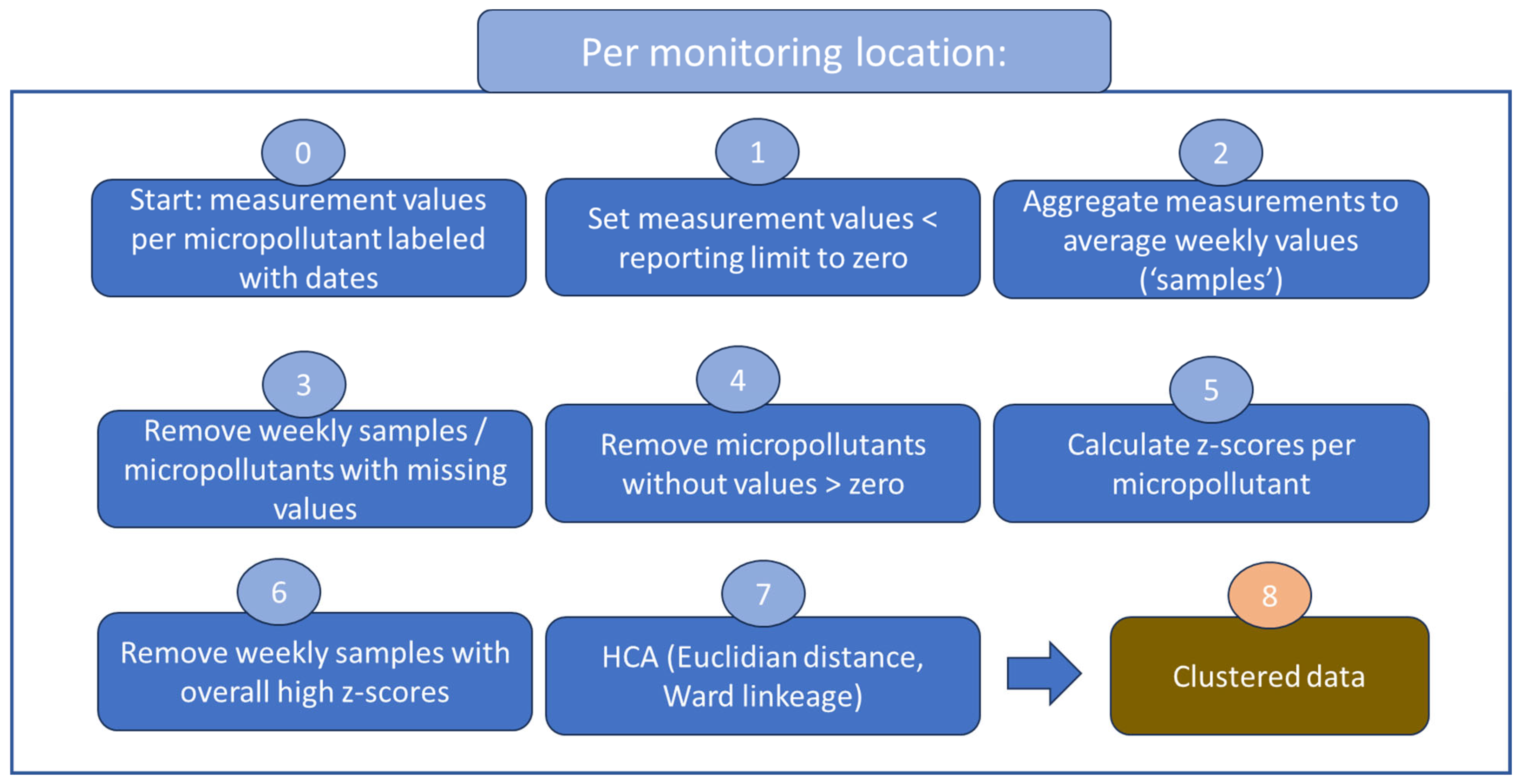
2.2. Cluster Analysis

Cluster analysis is a collection of different methods that group observations (here: concentrations of micropollutants) in clusters in such a way that the presence and concentration dynamics of micropollutants in the same cluster are more similar to each other than to those from other clusters. Hierarchical clustering (also called hierarchical cluster analysis or HCA) is a specific method of cluster analysis which builds a hierarchy of clusters. There is no prior information on group membership needed for HCA. The values of the substances’ concentrations in the weekly samples are used to compute similarity.

Weekly samples contained ‘missing values’ (meaning micropollutants were not analyzed in a sampling week). Missing values are not permitted in clustering, so we had to remove missing values while maintaining as much data as possible. For this, an algorithm was applied that automatically removed either the substance or the weekly sample with a relatively high fraction of missing values (step 3, Figure 1). This was repeated until the dataset no longer contained missing values. Locations that had <20 samples were subsequently omitted from the analyses. Additionally, substances that were only found at concentrations < RL were removed (step 4, Figure 1), as the absence of concentration dynamics hampers clustering.

To avoid giving more weight in the HCA to substances with higher concentrations (e.g., the concentration range varies over 3 orders of magnitude between metals and organic compounds), data were scaled using the Z-score (step 5, Figure 1). The Z-score is the number of standard deviations that a given data point lies from the mean. For data points that are below the mean, the Z-score is negative. The Z-score is calculated as:

$$\mathrm{Z}=\frac{(x-\mu )}{\sigma }$$

(1)

where x is the concentration of a given substance, μ it is the substances mean concentration, and σ is its standard deviation. Typically, Z-scores fall between −3 and 3.

Prior to clustering, weekly samples with exceptionally high Z-scores were excluded as ‘outliers’ because such deviating samples can disrupt regular patterns in clusters (step 6, Figure 1). This was conducted based on the visual inspection of dendrograms showing the hierarchical relationship between weekly samples. If a sample separated from the rest of the samples in the top of the hierarchy in the dendrogram, it was considered an outlier.

The function ‘hclust()’ in the statistical language ‘R’ was used to compute the hierarchical clusters (step 7, Figure 1). In this function, ‘Euclidean distance’ was used to estimate the (dis)similarity of each pair of substances or samples in the HCA. ‘Ward’ was used for determining how the distances should be interpreted to form hierarchical clusters. The Ward approach of clustering minimizes the within-cluster variance. This is in line with approaches applied in functional genomics data (e.g., [20]). Both the observations per micropollutant and the observations per weekly sample were clustered. Only the clusters per micropollutant were further analyzed.

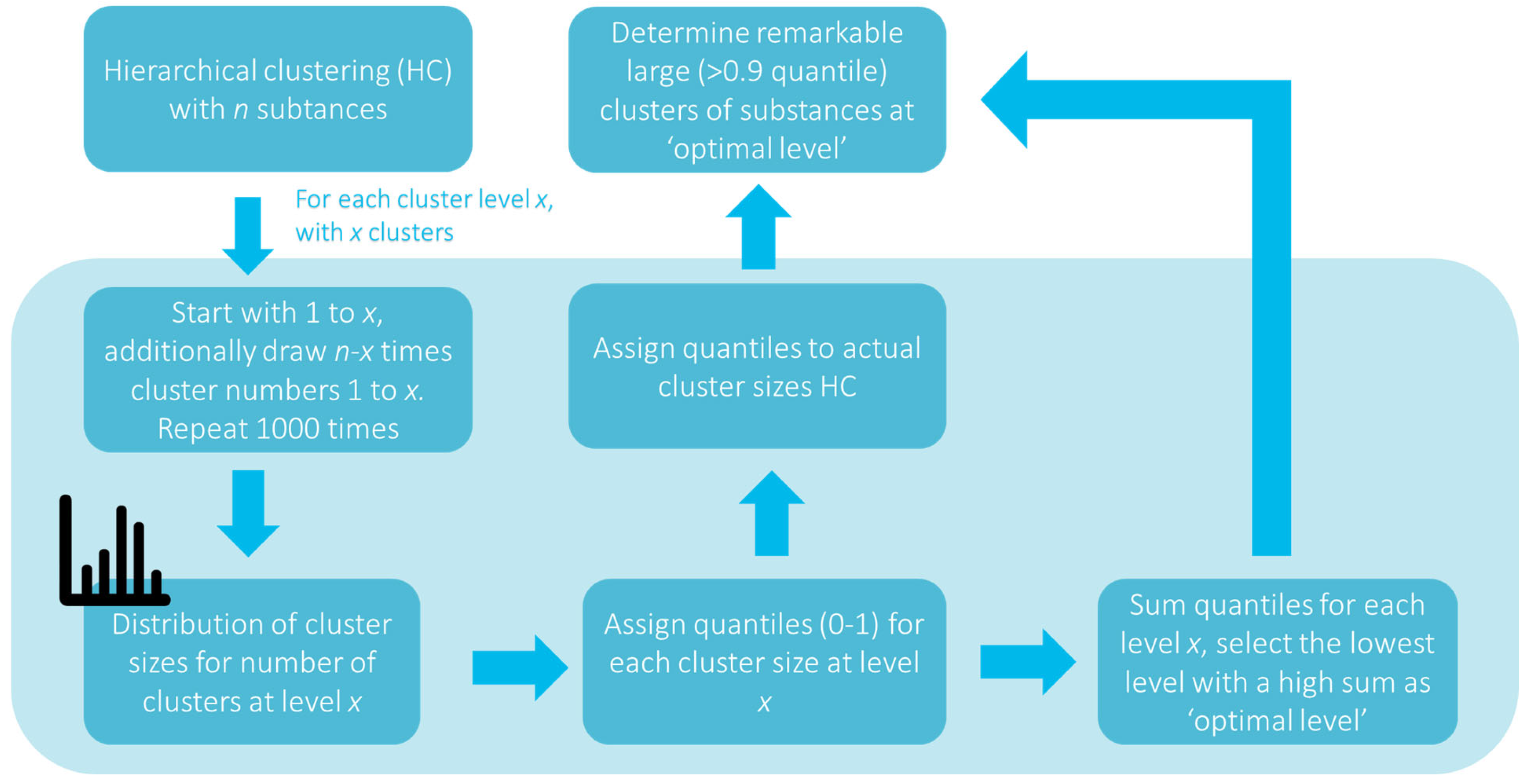
2.3. Assigning Cluster Significance

After the hierarchical clustering is computed, all substances are in a cluster at any level in the clustering hierarchy (e.g., dendrogram). Not all clusters contain highly similar (relative) concentrations. Therefore, a step is required to distinguish between clusters with low and high similar relative concentrations. It is necessary to define what specific clusters are relevant from all possible clusters. Rather than visually determining concise clusters, an approach to objectively point out such clusters was used. This was achieved by checking if, at a particular chosen level in the clustering hierarchy, clusters were larger than the 90 percentile in random expected cluster sizes at the given level. More details about the method can be found in Appendix C.

2.4. Overlap of Clusters with Reference Lists

The composition of the clusters was compared to several ‘reference lists’ (Appendix A) of substances. The reference lists were compiled using the literature data and (public) lists of substances (Appendix A,

Table A1. Sources of the reference substances lists, with numbers of sub-lists and substances per source.

List Source ID	List Source Name	Source	Sub-Lists	Sub-Stances
L1	Substances used in various agriculture types	Centraal Bureau voor de Statistiek	58	1715
L2	Substances measured near agriculture types	Landelijk Meetnet gewasbeschermingsmiddelen (data obtained from Deltares)	8	63
L3	Sewage treatment plants	Watson database (data driven, substances found >0.1 μg/L in >25 sewages’ effluents)	1	83
L4	Trans-border Meuse	RIWA database (data driven, substances in samples of location Eijsden on average >0.1 μg/L)	2	47
L5	Trans-border Rhine	RIWA database (data driven, substances in samples of location Lobith on average >0.1 μg/L)	2	71
L6	Biocides per product type	ECHA European Chemicals Agency database	20	656
L7	Distinguished groups (diverse)	RIWA-Rijn	89	1714
L8	Micropollutants as source and process indicators	[10]	17	71
L9	EU emissions by industries	EEA Industries Reporting Database	20	128
L10	Veterinary pharmaceuticals in manure slurries	[32]	2	28
L11	Sources of PFAS in Dutch surface water	[33]	11	13
L12	Typical substances in untreated wastewater	Watson database (data driven, substances found abundantly (>25 sewages’, at least 0.1 μg/L) in influent, not in effluent, and are well removed (>80%))	1	9
L13	Drug waste constituents	[34]	1	62
L14	A list of substances in fertilizers	CompTox lists	1	22
L15	Motor fuel leakage substances	CompTox lists	1	27
L16	Natural toxins	CompTox lists	1	90
L17	Veterinary drugs	CompTox lists	1	124
L18	Cyanoginosins (from cyanobacteria)	CompTox lists	1	7

). The reference lists are of a varying size and specificity (from general ‘micropollutants in wastewater treatment’ to specific ‘veterinary pharmaceuticals found in manure’).

A total of 232 separate lists were collected, including 1968 unique substances. Some of these lists show a high degree of overlap. This complicates the interpretation. Therefore, the lists were merged to avoid overlap. Two lists were merged if the sum of the percentage overlap of the two lists exceeded 130%. For instance, if list A has a 40% overlap with list B, and list B has 100% overlap with list A, together this sums up to 140% combined overlap. All reference lists were checked for overlap against all other reference lists. The merge resulted in a reduction to 164 separate reference substance lists. The overall similarity of the new reference lists (expressed as the % remaining overlap of substances) is visualized as a hierarchical clustering in Appendix A, Figure A1.

A hypergeometric test is used to quantify the significance of overlap between substances found in clusters and substances present in reference lists. This test is available as the function ‘phyper’ in the statistical language ‘R’. This method tests for significant overlap of two lists, resulting in a p-value for significance of the overlap (see Figure 2). This test is frequently used in genomics research to link gene expression patterns to known gene expression pathways [20] and is termed ‘enrichment analyses’ in that domain. The information that is required as input for this method is:

• M, the total number of relevant substances (in all reference lists and monitoring data);
• n, the substances in a reference substance list;
• N, the number of substances in a cluster;
• X, the number of substances in the overlap.

The probability of drawing X substances out of N from a measurement containing n reference substances out of all substances, M, can be computed with the phyper function in R the following way: p-value = phyper (x − 1, M, n, N).

If the overlap between a given reference list and a given cluster is larger than what is randomly expected, the p-value is low. The p-value is reported only if two or more substances overlap between the cluster and the reference list.

2.5. Linking Clusters to Substance Properties

Clusters were also analyzed with respect to their link to the physicochemical properties of the substances (e.g., solubility, K_OC, Henry’s constant, etc.). Such properties of substances were retrieved from (open source) models [22,23]. Inorganic substances were excluded from this analysis, as their properties were not always suitable for the models used for analysis. The retrieved properties of substances in each cluster were visualized with boxplots. Property values of substances within a cluster were compared to the distribution of the property value over all substances in all clusters, and the difference was tested with a t-test. The p-values were corrected for multiple testing using a Benjamini–Hochberg correction for the false discovery rate. Clusters were visualized only if these contained a minimum number of 4 organic substances. This number was chosen to avoid chance differences while retaining sufficient clusters.

2.6. Linking Clusters to Environmental Conditions

Information on environmental conditions was also linked to the observed clusters. These were river water conditions as reported in the RIWA datasets like oxygen, discharge, pH, dissolved organic carbon (DOC), and temperature as well as weather conditions that were downloaded from the Dutch Knowledge Institute for Weather, Climate, and Seismology KNMI (precipitation, sunny hours per day, and evaporation potential). Each monitoring location in Rhine and Meuse was linked to the closest weather station and weather data were aggregated per week by taking the mean.

Relating environmental conditions to clusters requires a rather complex analysis. First, normalization of the concentration values between locations was applied to account for structurally higher or lower concentrations of a substance in locations within the same river system. Then, per substance, it was identified which weekly samples had relatively high (top ten percent) concentration values over all locations (for Rhine and Meuse separately). For the identified weekly samples, the value of the environmental condition in the corresponding week and weather station was administrated. Then, the mean was taken of the administered environmental condition. This resulted in a single value of the condition that is associated with high concentrations of a substance in the cluster. In this way, per cluster, as many values were calculated as there were substances in the cluster. In short, the environmental condition values in the clusters represent the conditions under which concentrations of substances in the clusters are high. Boxplots visualize the substances’ environmental condition values per cluster, for Meuse and Rhine separately. It was tested for every cluster if the environmental condition values in a cluster were different (p < 0.01) from the condition values over all weeks and weather stations associated with clusters, with a t-test. The p-values were corrected for multiple testing by a Benjamini–Hochberg correction for the false discovery rate. Clusters were visualized only if these values contained a minimum number of 4 (organic or inorganic) substances to enable easy visual comparison with substance properties of clusters.

2.7. Identifying Significant Clusters That Are Recurring in Multiple Locations

Clusters are considered ‘recurring’ if they contain mostly the same substances in at least three individual significant clusters between locations. This was evaluated by an initial analysis of percentage overlap of the substances between clusters, and this was doublechecked by hand.

3. Results

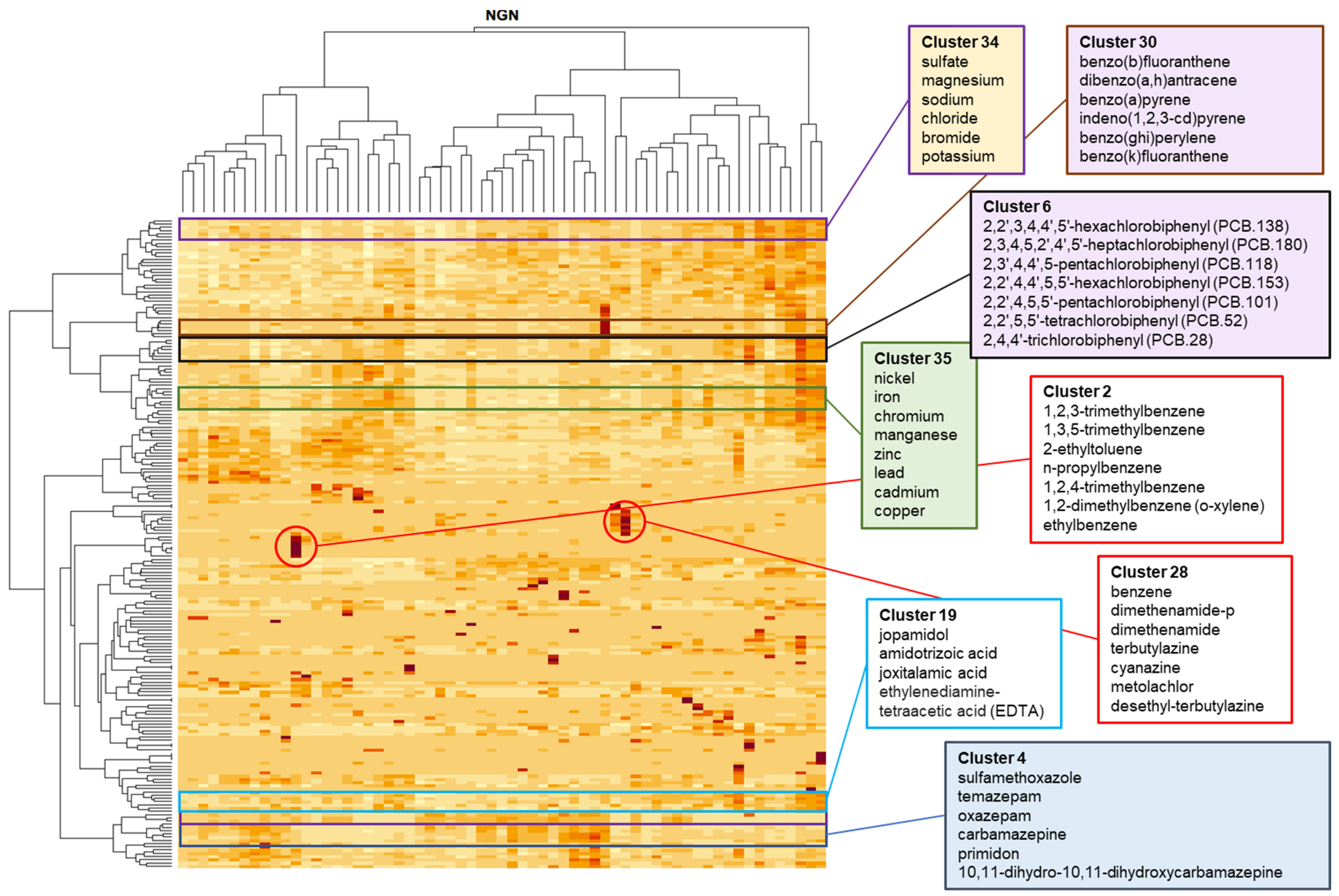
3.1. Clusters in Meuse and Rhine Locations

About ten significant clusters were found per location. An average significant cluster contained six substances. An overview is presented in Table 2. All significant clusters and the substances in them can be found in the data package associated with this paper. Some substances never occurred in a significant cluster, such as acetaminophen (paracetamol, painkiller) and trichloroacetic acid (among other uses, is a topical application against warts). In contrast, other substances were (if reported) always a member of a significant cluster at all locations, such as titanium (a metal) or indeno(1,2,3-cd)pyrene (a polycyclic aromatic hydrocarbon (PAH)).

As an example, the results of the clustering analysis in location Nieuwegein (Rhine) are shown in a heatmap (Figure 3). In this figure, the substances are in rows and the weekly samples are columns. Colors in the heatmap indicate the Z-scores of the measured concentrations per substance, from below the mean to above the mean concentration in increasingly darker color. Dendrograms indicate the hierarchy of clusters for weekly samples (at the top) and substances (at the left).

Some significant clusters of, in some way, similar substances were found, such as Polychlorinated Biphenyls (PCBs) (cluster 6), Polycyclic aromatic hydrocarbons (PAHs) (cluster 30), salts and reactive metals (cluster 34), metals (cluster 35), a cluster with mostly X-ray contrast agents (cluster 19), and a cluster with pharmaceuticals (cluster 4). These are indicated in Figure 3 by the boxes next to the heatmap. In Nieuwegein, some distinct clusters occurred in only one or two weekly samples, indicating an episodic discharge or emission. Some of these clusters are associated with agricultural applications (i.e., pesticides, insecticides, herbicides, and fungicides (cluster 28) or petrochemicals (cluster 2)). These example clusters are indicated in Figure 3 by the boxes next to the heatmap.

3.2. Overlap of Clusters with Reference Lists

For the remainder of this paper, ‘clusters’ refers to significant clusters. Overall, 57 out of 164 reference lists (see Appendix A) were significantly overlapping in one or more clusters in the Meuse and Rhine.

Table 3. Top five significantly overlapping (‘enriched’) reference lists in clusters from both Meuse (total 80 clusters) and Rhine (total 116 clusters). See Appendix A for an overview of all reference lists.

Reference Lists	Meuse Clusters	Rhine Clusters
‘Dutch Rivers’	29	48
‘Wastewater treatment plant’	33	43
‘Installations for waste processing or landfills or refinery’	19	23
‘Polycyclic aromatic hydrocarbons (PAHs)’	12	17
‘Industrial substances (containing PCBs)’	4	12
‘Herbicides based on a triazine group’	9	9

shows the top five significantly overlapping reference lists in the Rhine and Meuse clusters.

Most of the clusters overlapped with wastewater processing-type reference lists. This was expected for these rivers because they carry a high percentage of wastewater effluent. Also, the reference list, ‘Dutch rivers’, was logically found enriched often because it contains substances that are structurally found in the Meuse and Rhine. More specific reference lists that are often enriched are ‘Polycyclic aromatic hydrocarbons (PAHs)’, ‘Industrial substances (containing PCBs)’ and ‘Herbicides based on a triazine group’. It appears from this analysis that both rivers are, for the larger part, similarly affected.

Some smaller differences could be observed between the Rhine and Meuse. Some reference lists were uniquely (twice or more) overlapping significantly only with clusters of the Meuse. These were reference lists Greenhouse-potted plants (Gerbera and Chrysanthemum, Orchids), and Herbicides. For the Rhine, uniquely overlapping lists with clusters were Herbicides based on anilides, organochlorine-based insecticides, and nutrients. Of course, nutrients are present in the Meuse; however, these apparently do not cluster together to the extent that they do in the Rhine. Overall, the impression is that the association of clusters with reference lists is quite similar between Rhine and Meuse.

3.3. Recurring Clusters of Pollution

Some clusters are recurring in similar compositions at multiple sampling locations. This can be expected as the sampling locations are not independent within a river catchment and the substances in clusters can share sources, emission routes, applications, physicochemical properties that make them occur together, and follow similar temporal patterns. These clusters are referred to as ‘recurring clusters’ (

Table 4. Recurring clusters in the Meuse and Rhine. See Table 2 for abbreviations of locations. See the data package for substances associated with each of the cluster location codes.

Recurring Cluster Number	Substances	3 Example Clusters in Locations	Description
RC1	Aluminum, barium, beryllium, cadmium, cesium, chromium, iron, cobalt, copper, mercury, lithium, lead, manganese, rubidium, thallium, tin, titanium, vanadium, zinc, nickel, arsenic	LOB_20 NGN_18 MMM_5	Metals Sometimes combined with PAH substances
RC2	Boron, calcium, chloride, potassium, lithium, magnesium, molybdenum, sodium, rubidium, strontium, sulfate, uranium, bromide, silicate as Si	NGN_34 BRI_1 KAM_14	Salts and reactive (alkali) metals
RC3	benzo(a)anthracene, benzo(a)pyrene, benzo(b)fluoranthene, benzo(ghi)perylene, benzo(k)fluoranthene, chrysene, dibenzo(a,h)anthracene, fluoranthene, indeno(1,2,3-cd)pyrene, pyrene, phenanthrene, anthracene	LOB_22 NGN_30 EYS_8	Polycyclic aromatic hydrocarbons (PAHs) (fossil fuel burning) In some clusters together with PCBs like VWZ_4, HAV_21
RC4	Cyanazine, desethyl-terbutylazine, dimethenamide, dimethenamide-p, metolachlor, terbuthylazine, ethofumesate, metobromuron, linuron	NGN_28 NSL_20 BRA_28	Herbicides
RC5	2,2′,3,4,4′,5′-hexachlorobiphenyl (PCB 138), 2,2′,4,4′,5,5′-hexachlorobiphenyl (PCB 153), 2,2′,4,5,5′-pentachlorobiphenyl (PCB 101), 2,2′,5,5′-tetrachlorobiphenyl (PCB 52), 2,3′,4,4′,5-pentachlorobiphenyl (PCB 118), 2,3,4,5,2′,4′,5′-heptachlorobiphenyl (PCB 180), 2,4,4′-trichlorobiphenyl (PCB 28)	NGN_6 KMW_4 BRA_38	Polychlorinated Biphenyls (PCBs) (industrial and commercial applications)
RC6	1,2-dimethylbenzene (o-xylene), 1,2,4-trimethylbenzene, Benzene, Ethylbenzene, methylbenzene (toluene), 1,2,3-trimethylbenzene, 1,3,5-trimethylbenzene, 2-ethyltoluene, Ethenylbenzene, n-propylbenzene	KAM_2 NGN_2 KEI_1	Aromatic hydrocarbons (petrol oil and fuel)
RC7	10,11-dihydro-10,11-dihydroxycarbamazepine, carbamazepine, oxazepam, primidone, sulfamethoxazole, temazepam	NGN_4 AND_2 BRA_16	Pharmaceuticals
RC8	Amidotrizoic acid, ethylenediaminetetraethanoic acid (EDTA), jopamidol, joxitalamic acid jopromide, johexol	LOB_21 NGN_19 BRA_14	Contrast-agents
RC9	Bisoprolol, guanylureum, sotalol, hydrochlorothiazide, atenolol, metoprolol	AND_17 BRA_21 LOB_18	Beta blockers, diuretics

).

Many of the significant clusters (Table 2) are actually recurring clusters (Table 4). In total, 74 clusters (of which 64 clusters contain more than four substances) are identified as one of these recurring clusters. Substance properties and conditions that are associated with recurring clusters are of particular interest because properties and conditions may cause the substances to have similar concentration dynamics in different locations. In the following paragraphs, the recurring clusters are further analyzed.

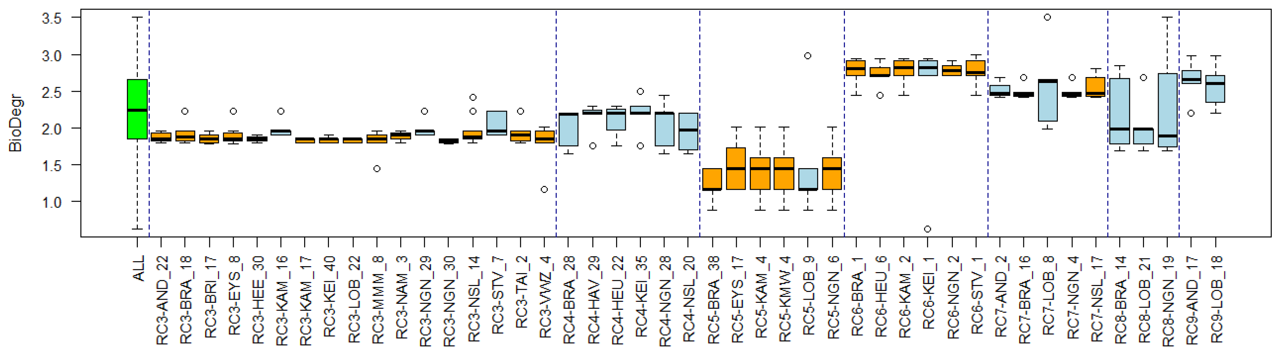
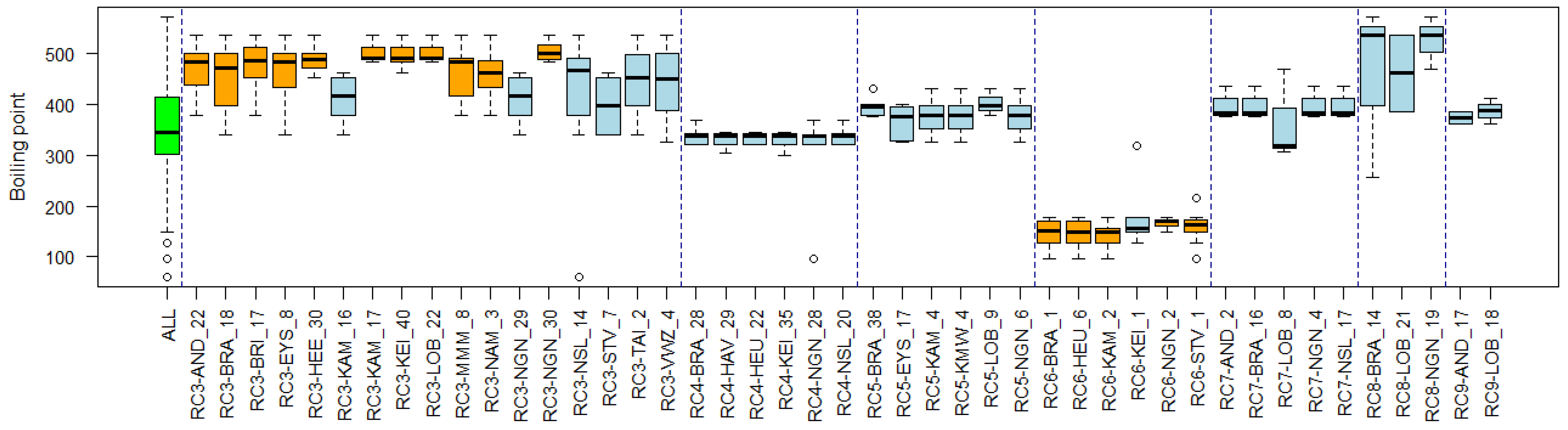
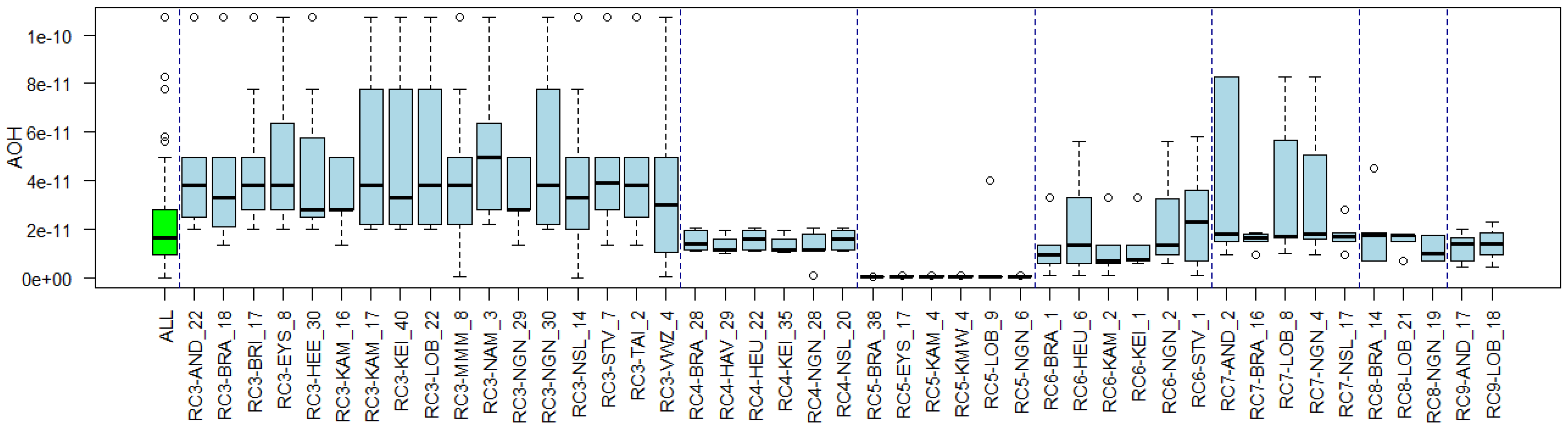
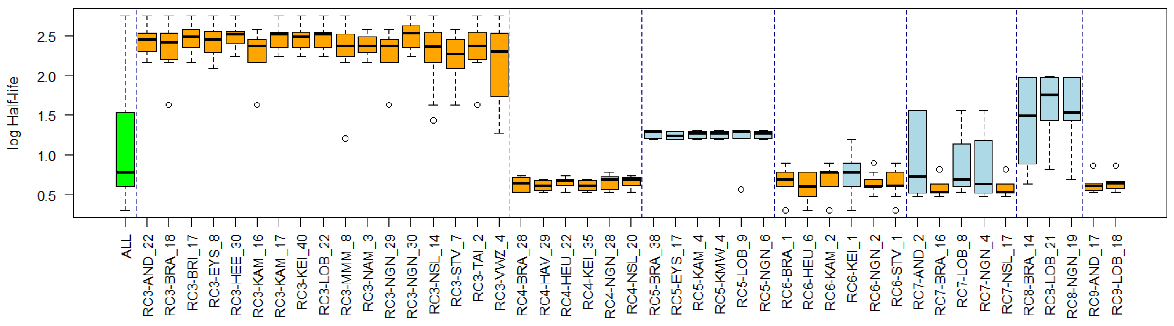
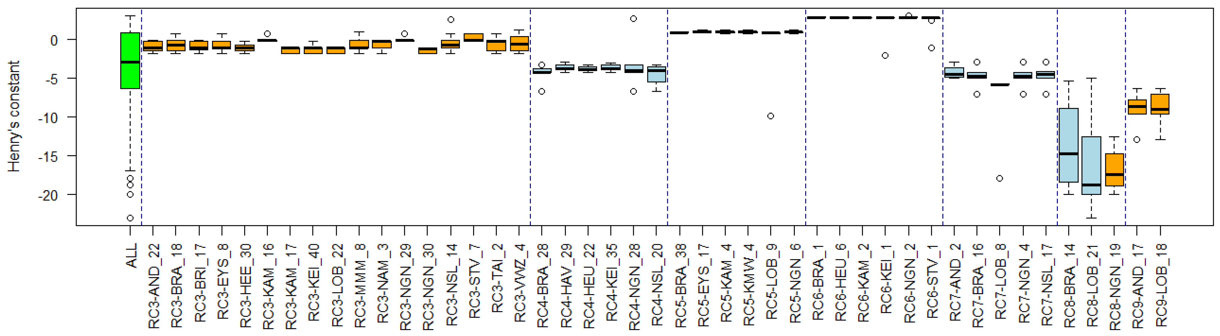
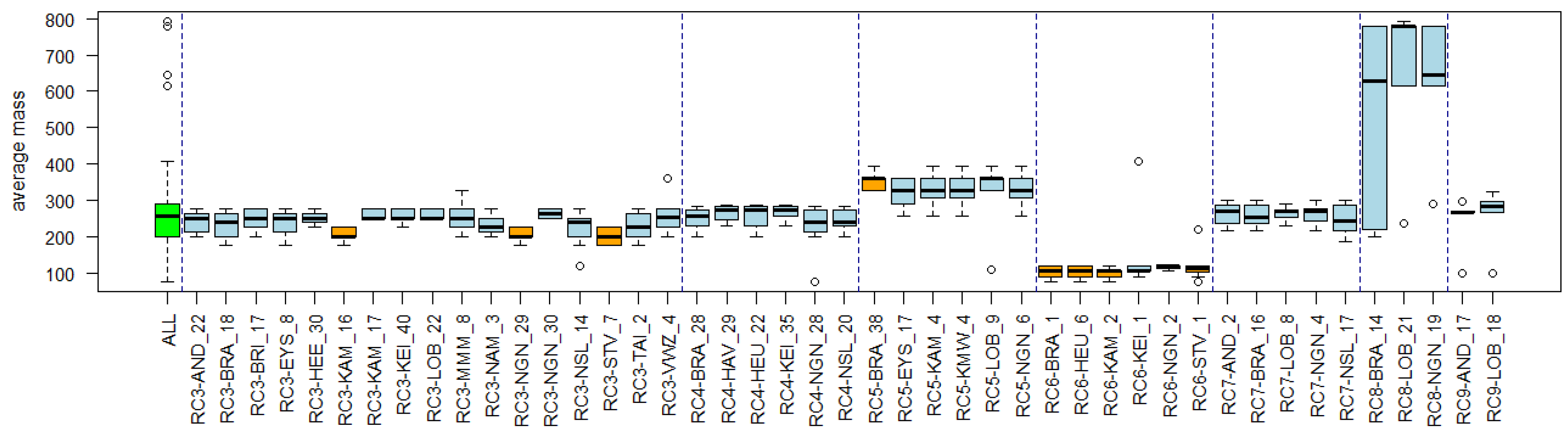
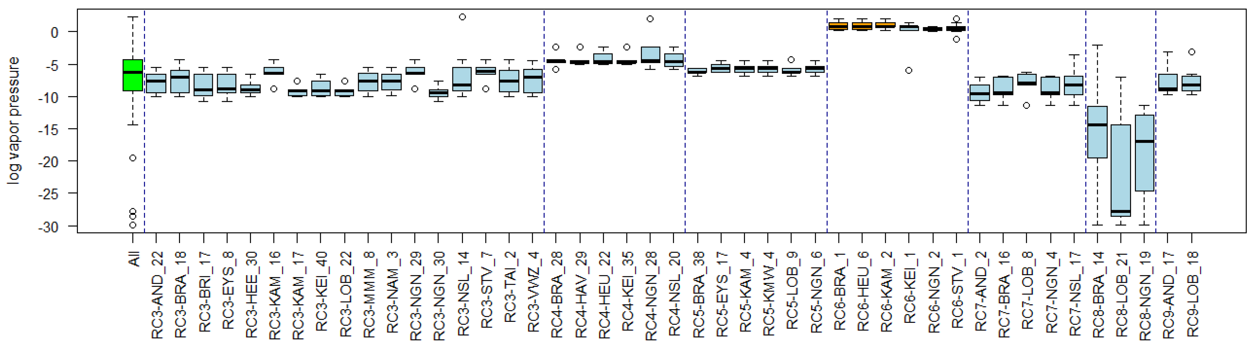
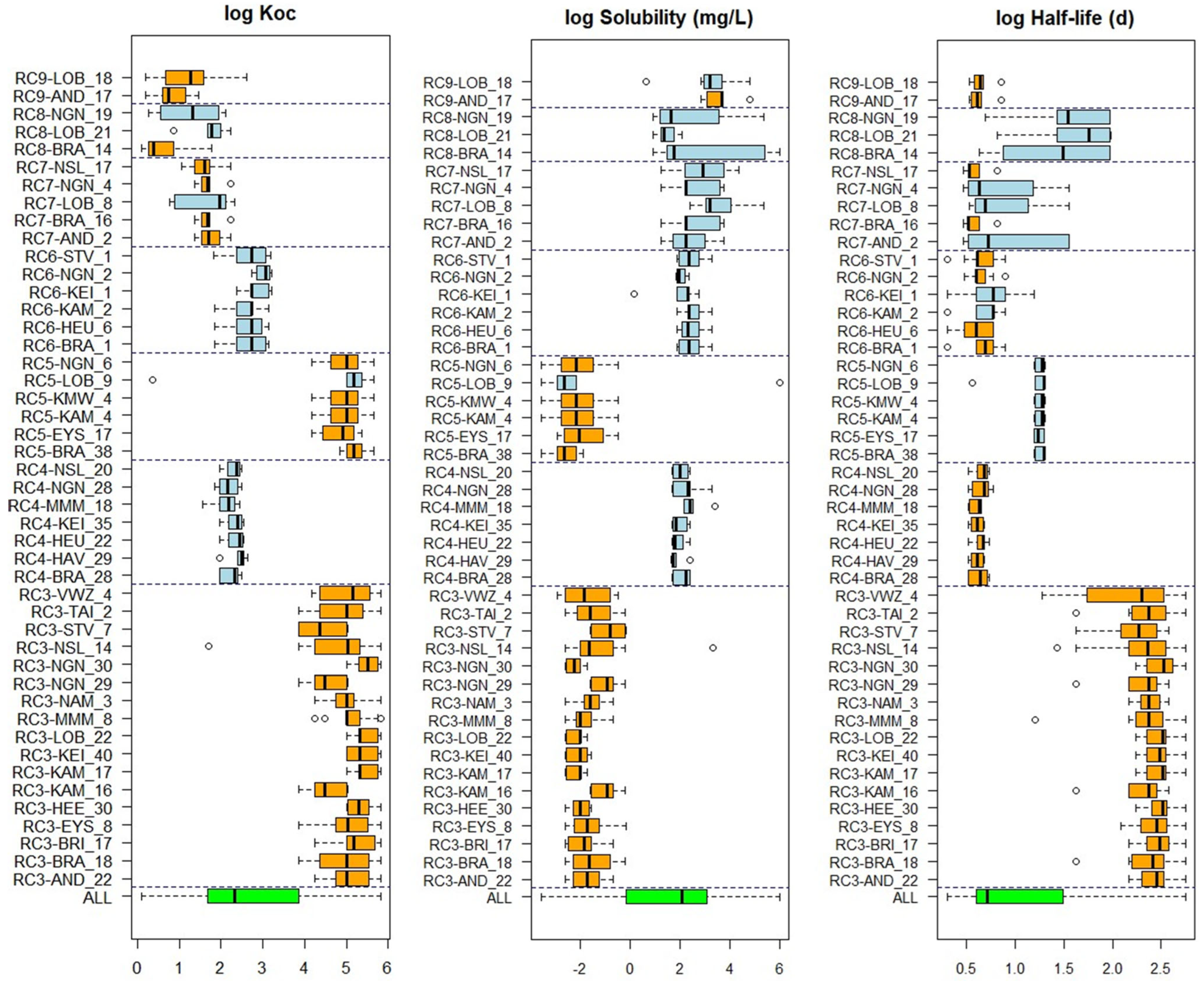
3.4. Substance Properties of Recurring Clusters

Figure 4 shows substance properties with which recurring clusters are most clearly and often (in many clusters) associated. These are logK_OC, logSolubility and logHalf-life. Clusters of substances with significantly deviating substance property values from the average green boxplot are indicated in orange. The results of all the considered substance properties are in Appendix B. The recurring clusters RC1 and RC2 are not shown because their properties cannot be calculated with the models used [22,23].

Another property that showed, relatively, many deviations from the average value in clusters was Henry’s constant (Appendix B). For this property, the clusters contained substances with significantly higher-than-average Henry’s constant, and only RC8 and RC9 tended to have lower-than-average values.

Other properties such as vapor pressure, average mass, atmospheric hydroxylation rate (AOH), and density were occasionally, but not structurally, significantly different for clusters (Appendix B). The associations of each recurring cluster with substance properties are summarized in

Table 5. Recurring clusters (see Table 4) with significantly overlapping reference lists, associated substance properties and environmental conditions. Enriched reference lists are separated by ‘/’. When no river name is mentioned for environmental conditions, both river systems apply.

Cluster Name	Overlapping Reference Lists	Substance Properties	Environmental Conditions
RC1 Metals	Dutch Rivers/ Installations for waste processing or landfills or refinery/ Wastewater treatment plant/Untreated wastewater Netherlands	n.a.	- low temperature - high discharge (Meuse) - high oxygen - high DOC - low evaporation potential - high precipitation (Meuse) - low pH (Rhine)
RC2 Salts, reactive metals	Dutch Rivers/ Wastewater treatment plant/Installations for waste processing or landfills or refinery	n.a.	- low discharge - high temperature (Meuse) - high sun hours (Meuse) - high evaporation potential (Meuse) - low precipitation (Meuse) - low oxygen (Meuse)
RC3 PAHs	Polycyclic aromatic hydrocarbons (PAHs)/Untreated wastewater Netherlands	- low solubility - high KOC/KOW - high half-life - low biodegradation - high Henry’s constant	- low temperature - high discharge (Meuse) - high oxygen (Meuse) - low evaporation potential (Meuse) - low sun hours (Meuse) - high precipitation (Meuse) - low pH
RC4 Herbicides	Herbicides based on a triazine group/Herbicides based on amides	- low half-life	- high temperature - low oxygen - high evaporation potential - low discharge (Meuse)
RC5 PCBs	Industrial substances (containing PCBs)	- low solubility - high KOC/KOW - medium-high half-life - low biodegradation - high Henry’s constant - low AOH	- low/medium temperature (Meuse) - low discharge (Rhine) - low evaporation potential (Meuse)
RC6 AHs	Petrol additives/Industrial solvents/Motor fuel leakage/Industrial substances	- low half-life - high biodegradation - high Henry’s constant - high Vapor Pressure - low KOA - low density/average mass - low melting point	- low DOC (Meuse)
RC7 Pharmaceuticals	Pharmaceuticals/Wastewater treatment plant/Exchange between surface and groundwater/Domestic wastewater/Antidepressants and narcotics	- low KOC - medium/high biodegradation	- low discharge
RC8 Contrast agents	Contrast agents/Domestic wastewater/Dutch Rivers/Wastewater treatment plant	- low to median KOC/KOW - low henry’s constant - medium-high half-life	- low discharge (Meuse)
RC9 Beta blockers	Blood pressure relievers and diuretics/ Dutch Rivers/ Wastewater treatment plant	- low half-life - high solubility - low KOC - low henry’s constant	- low temperature - high oxygen - low evaporation potential - low sun hours

.

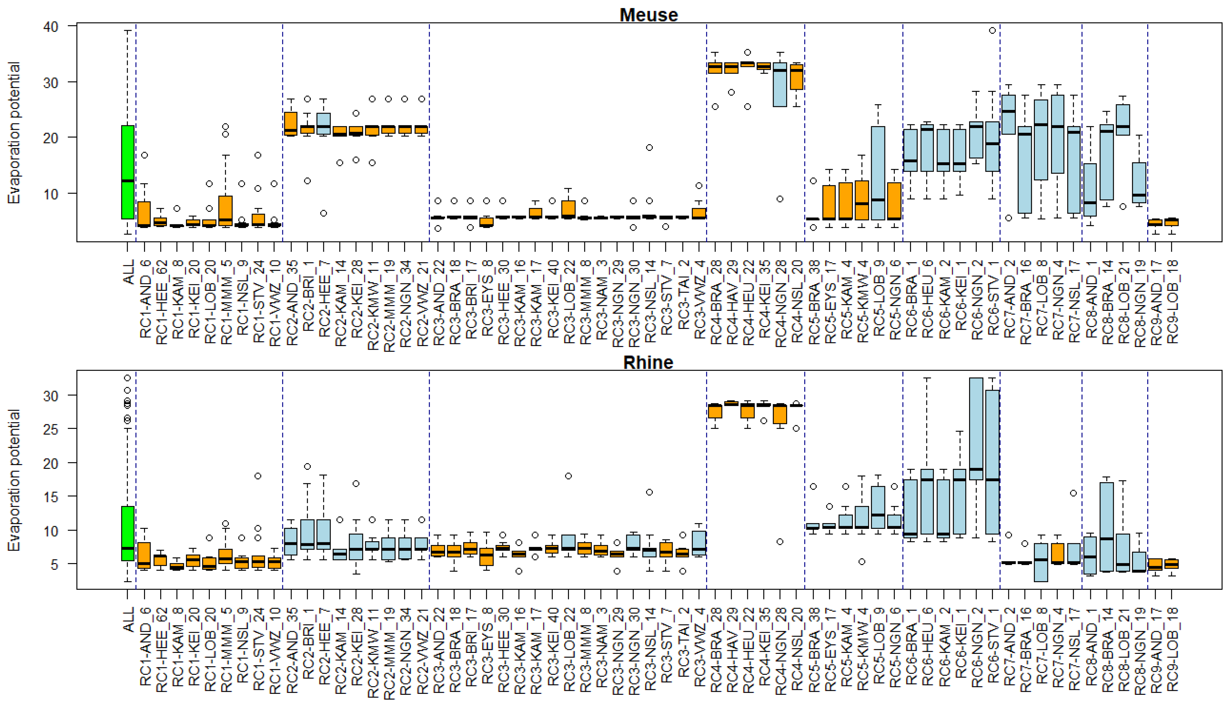
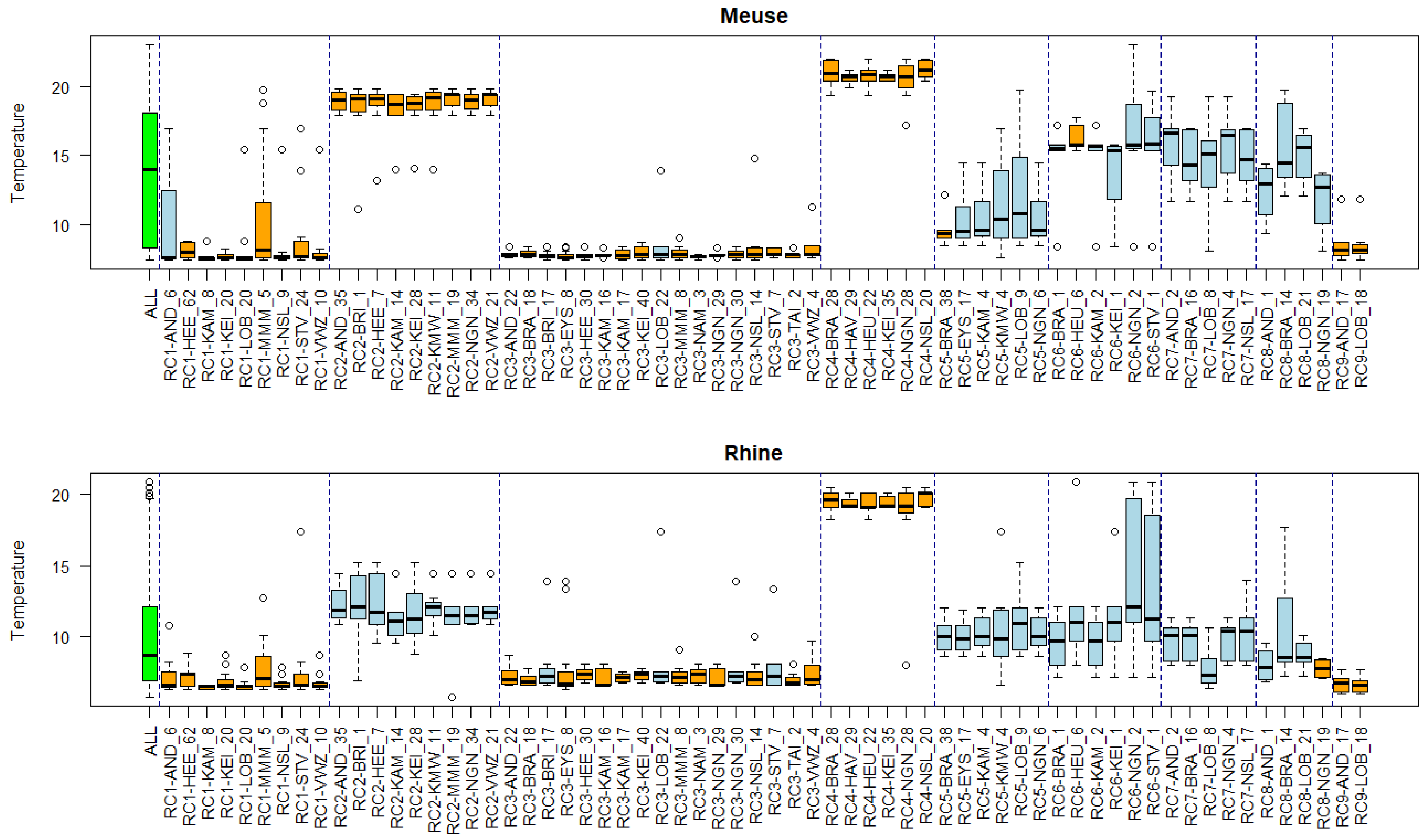
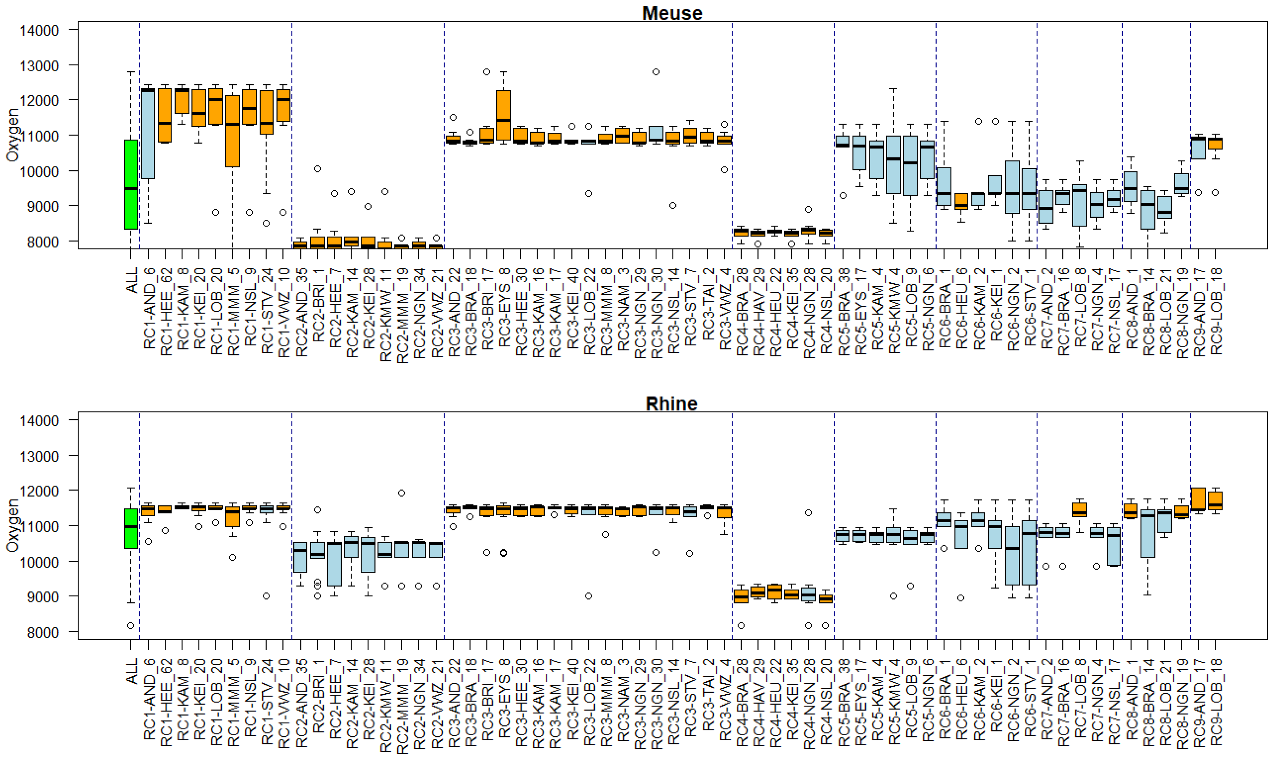
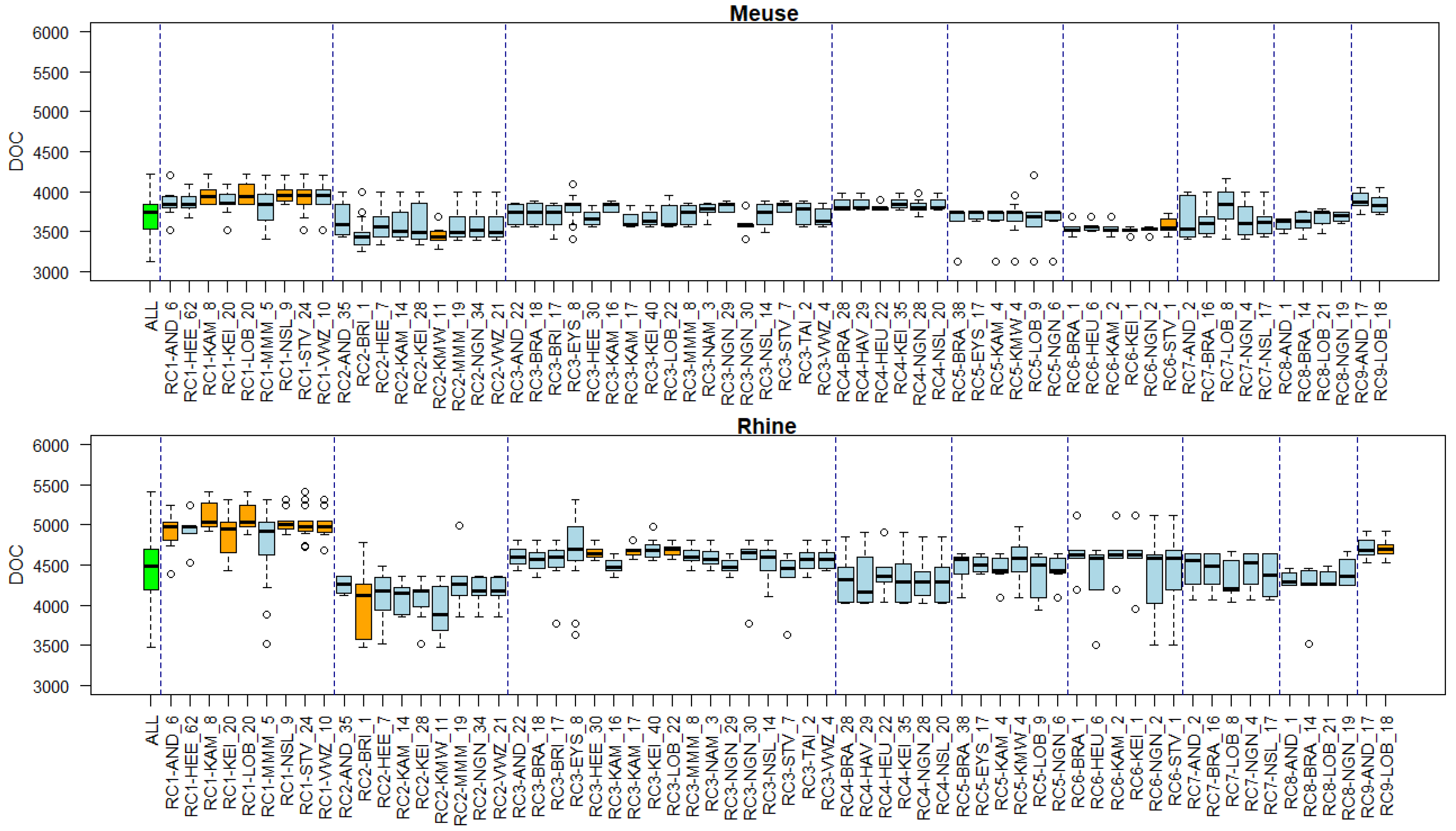
3.5. Associations of Environmental Conditions with Clusters

In Figure 5, three environmental condition values associated with high concentrations of substances in the recurring clusters are shown for the Meuse. The results of all analyses (Rhine and Meuse) are in Appendix B.

Figure 5 shows that several (indicated in orange) of the recurring clusters are associated with the environmental conditions temperature and river discharge values. Dissolved organic content (DOC) is less convincingly associated. A summary of all associations of repeating clusters with environmental conditions is given in Table 5. Other (related) conditions were associated with the clusters as well, such as high precipitation, oxygen level, evaporation potential, and less convincingly, pH (Appendix B).

Significantly associated reference lists, substance properties, and environmental condition are summarized in Table 5 for each recurring cluster (RC1–9).

Clusters of RC1 (‘metals’) are associated with environmental conditions, high DOC, and winter related conditions such as low temperature and high discharge. Clusters of RC2 (‘salts and (alkali) metals’) are associated with low discharge and summer-related conditions such as high temperature and sun hours, mainly in the river Meuse. Clusters of RC3 (PAHs) are associated with winter conditions, low mobility (high Koc and low solubility), high persistence, and high volatility potential. Clusters of RC4 (herbicides) are associated with low persistence (short half-life) and summer conditions. Clusters of RC5 (PCBs) are associated with substance properties similar to RC3 and winter-related conditions such as ‘low temperature’ and ‘low evaporation potential’. In the Rhine, clusters of RC5 are associated with low discharge; however, that does not necessarily fit with the ‘low temperature’ because discharge is generally high in winter when temperatures are low. Clusters of RC6 (‘Petrol additives/Industrial solvents/Motor fuel leakage/Industrial substances’) are associated with substance properties, like non-persistency (short half-life), low density, and high volatility potential (Henry’s constant and Vapor pressure) but no specific environmental conditions. Clusters of RC7 and RC8, which consist of pharmaceuticals and contrast agents, are associated with low discharge and high mobility (low to median K_OC). Clusters of RC9 (‘beta-blockers and diuretics’) are associated with high mobility (high solubility and low K_OC) and low volatility potential (low Henry’s constant), and with winter-like environmental conditions.

4. Discussion

In this study, unbiased statistical tools were applied on a wide variety of chemical water quality parameters obtained from regularly monitoring activities at multiple locations in the river Rhine and Meuse. These river systems were chosen because of the large monitoring datasets, with frequent measurements of many different parameters. The rivers Rhine and Meuse integrate many sources of pollution with many emission routes. The aim was to extract valuable (and often overlooked) information from these datasets and explain clustering of substances by their co-occurrence, association to substance properties, environmental conditions, and possible emission.

Based on concentration dynamics in five years of monitoring data, multiple significant clusters of substances were found for each of the nineteen locations in the Meuse and Rhine. A large portion of such clusters could be statistically linked to a combination of substance properties, environmental conditions, and had significant overlap with emission-related reference lists of substances with a common application, origin, and/or chemical class. Environmental scientists can interpret the observations, bringing the unbiased approach and the mechanistic understanding based on prior knowledge together. Dedicated measurements and experiments are needed to confirm these statistical links for the different clusters containing (groups of) micropollutants.

Several substance properties proved to be significantly associated with clusters. It is well known that the fate of substances in a river catchment is affected by properties [24]. Even if the associated properties are not new with regard to fate (e.g., [24]), the found combinations of associated substance properties in clusters exemplify their role in concerted concentration dynamics in the rivers. The solubility, K_OC, half-life, and Henry’s coefficient of substances deviated from the average value in many clusters. Solubility provides an important indication of a contaminant’s mobility in the aquatic environment. A high solubility makes a substance remain in the aqueous phase. The tendency of a substance to migrate from water to air is expressed by Henry’s law constant. A high value means a high potential for volatilization. K_OC is a measure for the expected distribution of a substance between a solid phase such as soil or sediment and water. It determines whether the substance will accumulate in sediments, travel with the aqueous phase or travel with suspended particles (if present) in the aqueous phase. A low K_OC implies that the substance is mobile. The octanol (oily organic solvent) water partition coefficient (K_OW) is used as a surrogate, since it is easier to determine/available for many substances. Lastly, the half-life of substances indicates their persistence in the (aqueous) environment. Actual half lives in the field are very conditional, depending on temperature, redox conditions, sorption, and presence of (micro) organisms that are able to degrade the substance of interest. A longer half-life allows a chemical to travel further away from its sources and increases the possibility to encounter the chemical long after it has been emitted.

Environmental conditions affect the fate of chemicals [1] dependent on their emission pathways and substance properties. Conditions significantly associated to a large portion of clusters were temperature and river discharge. These associations enable the formulation of hypotheses on the impact of environmental conditions on substance concentrations. For instance, a positive association with temperature could simply indicate seasonal emissions, but also could indicate an increased formation of some substances at higher temperatures or with more intense (sun)light [25]. Similarly, a negative association may, for some substances, be attributed to degradation [1]. At low river discharge, concentrations of chemicals that have stable emissions increase because there is less dilution. Sewage treatment-emitted substances are a typical example of such substances because their supply is independent of river discharge. Some conditions are very logically interconnected with each other like evaporation potential (based on radiation) and sun hours, or river discharge and rain. Similarly, temperature and oxygen are connected because more oxygen can be mixed in cold water. This means that an important next step is to find which condition actually drives concentration differences of substances in clusters, or how these add up. This was not investigated in this study.

Clusters of substances that simultaneously enter the water can become separated along the traveled distance mainly by degradation, differences in solubility, volatility, or the tendency to stick to sediment. If chemicals with a wide variety of properties such as solubility and K_OC cluster together, this might indicate that they share the same source and emission pathway and are continuously emitted and/or the sample location is close to the source.

With regard to the overlap of substances in a cluster with reference lists of substances, the results could not distinguish between Rhine and Meuse. Sampling locations at the lower parts of the river Rhine and Meuse are exposed to many (upstream) sources of contamination through many emission pathways. This mixes different emissions and makes the association of the sampling locations with very specific reference lists such as ‘insecticides’ or ‘motor fuel leakage’ less likely, whereas a more generic reference list such as ‘Domestic wastewater’, was found significantly associated to many clusters. By working with clusters of substances rather than all substances at once, we were able to have a significant overlap for individual clusters with several reference lists. These were indicative mainly of wastewater, industrial influence, and agricultural influence. Associating reference lists to pollution might be more suitable for smaller surface water catchments with more specific and limited emission routes and sources. This may also work well in groundwater aquifers that are, by nature, spatially more heterogenic and likely affected by single or limited numbers of contamination sources.

With the clusters, the substance properties, conditions, reference lists, and the actual temporal concentration variation over the samples, hypotheses can be formed for every cluster that is found. Some clusters reoccurred at multiple locations. Especially these recurring clusters appeared to be determined by environmental conditions. For the recurring clusters with metals, PAHs, and PCBs, for instance, these factors may point to resuspension from sediment, as these substances strongly sorb to sediments and co-occur with a high discharge [26,27]. For the recurring cluster with Herbicides, results point to an application in summer. The recurring cluster with pharmaceuticals and contrast agents in combination with low river discharge point to current and continuous emissions from sewage treatment plants [28]. This is not surprising, but it illustrates that the data supports these well-known pathways and might also help in identifying deviations from these trends, indicative of an event with increased pharmaceutical use like an influenza outbreak [29]. The recurring cluster with Aromatic hydrocarbons could not be linked to any environmental condition. This could point to an irregular incident emission, such as an oil spill [30].

While these results are promising, changing measurements below the reporting limit to zero may have introduced errors in the formation of clusters by changing the pattern of varying concentrations too much from the actual concentrations. This also advocates for the use of sensitive analytical techniques to allow studying the occurrence of substances in their full range of environmental concentrations, not only focusing on the highest concentrations that occasionally occur or are found at ‘hot spot’ locations. An option is to remove all measurements below RL to only maintain the accurately measured values. Because it is necessary to remove all incomplete weekly samples or substances for the clustering analyses, this would result in a very small dataset per location. Moreover, for most substances the values below RL are indeed real ‘near zero’ values. Nevertheless, especially incidentally clustering substances with many measurements, <RL should be critically assessed. It may be that imputing values < RL or applying other statistical techniques (e.g., [31]) may yield better clustering for such substances and this could be investigated in follow-up research.

Based on the results obtained in this investigation, this type of large-scale environmental forensic studies using statistical analysis and clustering appear to be useful for processing existing datasets and extracting information that would otherwise remain concealed within datasets. It can be concluded that monitoring data contain far more information than simply concentration levels that are used for assessing compliance with water quality guidelines. Clustering and the cooccurrence of certain types of substances and differences and similarities of locations provide a wealth of information for building and testing hypothesis on sources, emissions, and impact of conditions on concentrations and loads. With that, it provides an important piece in the iterative puzzle towards understanding concentration dynamics, sources, and their contributions and can even, in the future, support the formulation and evaluation of mitigation strategies.

References

1. Musolff, A.; Leschik, S.; Möder, M.; Strauch, G.; Reinstorf, F.; Schirmer, M. Temporal and spatial patterns of micropollutants in urban receiving waters. Environ. Pollut. 2009, 157, 3069–3077. [Google Scholar] [CrossRef]
2. Baragaño, D.; Ratié, G.; Sierra, C.; Chrastný, V.; Komárek, M.; Gallego, J.R. Multiple pollution sources unravelled by environmental forensics techniques and multivariate statistics. J. Hazard. Mater. 2022, 424, 127413. [Google Scholar] [CrossRef]
3. Liu, Y.; Chen, L.; Huang, Q.-H.; Li, W.-Y.; Tang, Y.-J.; Zhao, J.-F. Source apportionment of polycyclic aromatic hydrocarbons (PAHs) in surface sediments of the Huangpu River, Shanghai, China. Sci. Total Environ. 2009, 407, 2931–2938. [Google Scholar] [CrossRef] [PubMed]
4. Luo, T.; Hu, S.; Cui, J.; Tian, H.; Jing, C. Comparison of arsenic geochemical evolution in the Datong Basin (Shanxi) and Hetao Basin (Inner Mongolia), China. Appl. Geochem. 2012, 27, 2315–2323. [Google Scholar] [CrossRef]
5. Cha, Y.; Kim, Y.M.; Choi, J.-W.; Sthiannopkao, S.; Cho, K.H. Bayesian modeling approach for characterizing groundwater arsenic contamination in the Mekong River basin. Chemosphere 2016, 143, 50–56. [Google Scholar] [CrossRef] [PubMed]
6. Bonelli, M.G.; Ferrini, M.; Manni, A. Artificial neural networks to evaluate organic and inorganic contamination in agricultural soils. Chemosphere 2017, 186, 124–131. [Google Scholar] [CrossRef] [PubMed]
7. Cho, K.H.; Sthiannopkao, S.; Pachepsky, Y.A.; Kim, K.-W.; Kim, J.H. Prediction of contamination potential of groundwater arsenic in Cambodia, Laos, and Thailand using artificial neural network. Water Res. 2011, 45, 5535–5544. [Google Scholar] [CrossRef]
8. Brückner, I.; Classen, S.; Hammers-Wirtz, M.; Klaer, K.; Reichert, J.; Pinnekamp, J. Tool for selecting indicator substances to evaluate the impact of wastewater treatment plants on receiving water bodies. Sci. Total. Environ. 2020, 745, 140746. [Google Scholar] [CrossRef]
9. Jekel, M.; Dott, W.; Bergmann, A.; Dünnbier, U.; Gnirß, R.; Haist-Gulde, B.; Hamscher, G.; Letzel, M.; Licha, T.; Lyko, S.; et al. Selection of organic process and source indicator substances for the anthropogenically influenced water cycle. Chemosphere 2015, 125, 155–167. [Google Scholar] [CrossRef]
10. Warner, W.; Licha, T.; Nödler, K. Qualitative and quantitative use of micropollutants as source and process indicators. A review. Sci. Total Environ. 2019, 686, 75–89. [Google Scholar] [CrossRef]
11. Kahl, S.; Nivala, J.; van Afferden, M.; Müller, R.A.; Reemtsma, T. Effect of design and operational conditions on the performance of subsurface flow treatment wetlands: Emerging organic contaminants as indicators. Water Res. 2017, 125, 490–500. [Google Scholar] [CrossRef] [PubMed]
12. Wolf, L.; Held, I.; Eiswirth, M.; Hötzl, H. Impact of Leaky Sewers on Groundwater Quality. Acta Hydrochim. Hydrobiol. 2004, 32, 361–373. [Google Scholar] [CrossRef]
13. ter Laak, T.L.; Kooij, P.J.F.; Tolkamp, H.; Hofman, J. Different compositions of pharmaceuticals in Dutch and Belgian rivers explained by consumption patterns and treatment efficiency. Environ. Sci. Pollut. Res. Int. 2014, 21, 12843–12855. [Google Scholar] [CrossRef] [PubMed]
14. Buttiglieri, G.; Peschka, M.; Frömel, T.; Müller, J.; Malpei, F.; Seel, P.; Knepper, T.P. Environmental occurrence and degradation of the herbicide n-chloridazon. Water Res. 2009, 43, 2865–2873. [Google Scholar] [CrossRef] [PubMed]
15. Byer, J.D.; Struger, J.; Sverko, E.; Klawunn, P.; Todd, A. Spatial and seasonal variations in atrazine and metolachlor surface water concentrations in Ontario (Canada) using ELISA. Chemosphere 2011, 82, 1155–1160. [Google Scholar] [CrossRef] [PubMed]
16. Harman, C.; Reid, M.; Thomas, K.V. In Situ Calibration of a Passive Sampling Device for Selected Illicit Drugs and Their Metabolites in Wastewater, And Subsequent Year-Long Assessment of Community Drug Usage. Environ. Sci. Technol. 2011, 45, 5676–5682. [Google Scholar] [CrossRef] [PubMed]
17. Loraine, G.A.; Pettigrove, M.E. Seasonal Variations in Concentrations of Pharmaceuticals and Personal Care Products in Drinking Water and Reclaimed Wastewater in Southern California. Environ. Sci. Technol. 2006, 40, 687–695. [Google Scholar] [CrossRef]
18. Seitz, W.; Winzenbacher, R. A survey on trace organic chemicals in a German water protection area and the proposal of relevant indicators for anthropogenic influences. Environ. Monit. Assess. 2017, 189, 244. [Google Scholar] [CrossRef]
19. Pascual-Aguilar, J.; Andreu, V.; Picó, Y. An environmental forensic procedure to analyse anthropogenic pressures of urban origin on surface water of protected coastal agro-environmental wetlands (L’Albufera de Valencia Natural Park, Spain). J. Hazard. Mater. 2013, 263, 214–223. [Google Scholar] [CrossRef]
20. Hermsen, S.A.B.; Pronk, T.E.; van den Brandhof, E.-J.; van der Ven, L.T.M.; Piersma, A.H. Transcriptomic analysis in the developing zebrafish embryo after compound exposure: Individual gene expression and pathway regulation. Toxicol. Appl. Pharmacol. 2013, 272, 161–171. [Google Scholar] [CrossRef]
21. Pronk, T.E.; van Someren, E.P.; Stierum, R.H.; Ezendam, J.; Pennings, J.L.A. Unraveling toxicological mechanisms and predicting toxicity classes with gene dysregulation networks. J. Appl. Toxicol. 2013, 33, 1407–1415. [Google Scholar] [CrossRef] [PubMed]
22. Mansouri, K.; Grulke, C.M.; Judson, R.S.; Williams, A.J. OPERA models for predicting physicochemical properties and environmental fate endpoints. J. Cheminformatics 2018, 10, 1–19. [Google Scholar] [CrossRef] [PubMed]
23. US EPA. Estimation Programs Interface Suite™ for Microsoft® Windows; version 4.11; United States Environmental Protection Agency: Washington, DC, USA, 2023.
24. Mamy, L.; Patureau, D.; Barriuso, E.; Bedos, C.; Bessac, F.; Louchart, X.; Martin-Laurent, F.; Miege, C.; Benoit, P. Prediction of the Fate of Organic Compounds in the Environment From Their Molecular Properties: A Review. Crit. Rev. Environ. Sci. Technol. 2015, 45, 1277–1377. [Google Scholar] [CrossRef] [PubMed]
25. Li, J.; Gao, J.; Zheng, Q.; Thai, P.K.; Duan, H.; Mueller, J.F.; Yuan, Z.; Jiang, G. Effects of pH, Temperature, Suspended Solids, and Biological Activity on Transformation of Illicit Drug and Pharmaceutical Biomarkers in Sewers. Environ. Sci. Technol. 2021, 55, 8771–8782. [Google Scholar] [CrossRef] [PubMed]
26. Echols, K.R.; Brumbaugh, W.G.; Orazio, C.E.; May, T.W.; Poulton, B.C.; Peterman, P.H. Distribution of Pesticides, PAHs, PCBs, and Bioavailable Metals in Depositional Sediments of the Lower Missouri River, USA. Arch. Environ. Contam. Toxicol. 2008, 55, 161–172. [Google Scholar] [CrossRef] [PubMed]
27. Schneider, A.R.; Porter, E.T.; Baker, J.E. Polychlorinated Biphenyl Release from Resuspended Hudson River Sediment. Environ. Sci. Technol. 2007, 41, 1097–1103. [Google Scholar] [CrossRef] [PubMed]
28. Brunsch, A.F.; ter Laak, T.L.; Rijnaarts, H.; Christoffels, E. Pharmaceutical concentration variability at sewage treatment plant outlets dominated by hydrology and other factors. Environ. Pollut. 2018, 235, 615–624. [Google Scholar] [CrossRef]
29. Azuma, T.; Nakada, N.; Yamashita, N.; Tanaka, H. Synchronous Dynamics of Observed and Predicted Values of Anti-influenza drugs in Environmental Waters during a Seasonal Influenza Outbreak. Environ. Sci. Technol. 2012, 46, 12873–12881. [Google Scholar] [CrossRef]
30. Mu, G.; Bian, D.; Zou, M.; Wang, X.; Chen, F. Pollution and Risk Assessment of Polycyclic Aromatic Hydrocarbons in Urban Rivers in a Northeastern Chinese City: Implications for Continuous Rainfall Events. Sustainability 2023, 15, 5777. [Google Scholar] [CrossRef]
31. Helsel, D.R. More Than Obvious: Better Methods for Interpreting nondetect data. Environ. Sci. Technol. 2005, 39, 419–423. [Google Scholar] [CrossRef]
32. Rakonjac, N.; van der Zee, S.E.; Wipfler, L.; Roex, E.; Kros, H. Emission estimation and prioritization of veterinary pharmaceuticals in manure slurries applied to soil. Sci. Total Environ. 2022, 815, 152938. [Google Scholar] [CrossRef]
33. Jans, A.C.H.; Berbee, R.P.M. Sources of PFAS for Dutch Surface Waters. RWS Report. 2020. Available online: https://open.rijkswaterstaat.nl/publish/pages/135993/rws_information_sources_of_pfas_for_dutch_surface_waters.pdf (accessed on 2 January 2024).
34. van Leerdam, R.C.; van Driezum, I.H.; Broekman, M.H. Type De Gevaren Van Dumpingen en Lozingen Van Drugsproductieafval Voor de Kwaliteit Van Drinkwaterbronnen. RIVM Report. 2022. Available online: https://rivm.openrepository.com/handle/10029/626320 (accessed on 2 January 2024).
35. Suzuki, R.; Shimodaira, H. Pvclust: An R package for assessing the uncertainty in hierarchical clustering. Bioinformatics 2006, 22, 1540–1542. [Google Scholar] [CrossRef]
36. Kimes, P.K.; Liu, Y.; Neil Hayes, D.; Marron, J.S. Statistical significance for hierarchical clustering. Biometrics 2017, 73, 811–821. [Google Scholar] [CrossRef]
Figure 1. Workflow for preprocessing of the data per location for hierarchical clustering analyses (HCA), yielding substance clusters per location. A selection for ‘significant’ clusters follows after this workflow (not shown).
Environments 11 00046 g001
Figure 2. Visualization of the hypergeometric test for significance of enrichment of ‘reference list’ substances of any reference list in a cluster.
Environments 11 00046 g002
Figure 3. Heatmap obtained using monitoring data from Nieuwegein (NGN). Rows: substances. Columns: weekly aggregated monitoring samples (see Figure 1) between 2017–2021. Some example clusters are highlighted by a colored box. The substances are indicated attached to the box. Darker colors indicate higher relative concentrations (Z-score).
Environments 11 00046 g003
Figure 4. The association of recurring clusters (Table 4) with substance properties. The green box at the bottom indicates the average property value of all the substances in the analysis. Clusters are indicated on the y-axis by a recurring cluster code (see Table 4), a location code (see Table 2), and a cluster number. Orange boxplots are significantly different from the average property value (p < 0.01), blue boxplots are not. See the data package for substances associated with each of the coded clusters.
Environments 11 00046 g004
Figure 5. The association of recurring clusters with conditions. The green box indicates the condition values at high concentration of all the substances in all clusters. Clusters are indicated on the y-axis by a recurring cluster code (see Table 4), a location code (see Table 2), and a cluster number. Orange boxplots are significantly different from the average condition value (p < 0.01), blue boxplots are not. See the data package for substances associated with each of the coded clusters.
Environments 11 00046 g005