Effects of Class Purity of Training Patch on Classification Performance of Crop Classification with Convolutional Neural Network †


Department of Geoinformatic Engineering, Inha University, Incheon 22212, Korea
*
Author to whom correspondence should be addressed.
†
This paper is an extended version of paper published in the 40th Asian Conference on Remote Sensing (ACRS 2019), held in Daejeon, Korea, 14–18 October 2019.
Appl. Sci. 2020, 10(11), 3773; https://doi.org/10.3390/app10113773
Submission received: 25 April 2020
/
Revised: 20 May 2020
/
Accepted: 27 May 2020
/
Published: 29 May 2020
(This article belongs to the Special Issue Remote Sensing and Geoscience Information Systems in Applied Sciences)
Abstract
:As the performance of supervised classification using convolutional neural networks (CNNs) are affected significantly by training patches, it is necessary to analyze the effects of the information content of training patches in patch-based classification. The objective of this study is to quantitatively investigate the effects of class purity of a training patch on performance of crop classification. Here, class purity that refers to a degree of compositional homogeneity of classes within a training patch is considered as a primary factor for the quantification of information conveyed by training patches. New quantitative indices for class homogeneity and variations of local class homogeneity over the study area are presented to characterize the spatial homogeneity of the study area. Crop classification using 2D-CNN was conducted in two regions (Anbandegi in Korea and Illinois in United States) with distinctive spatial distributions of crops and class homogeneity over the area to highlight the effect of class purity of a training patch. In the Anbandegi region with high class homogeneity, superior classification accuracy was obtained when using large size training patches with high class purity (7.1%p improvement in overall accuracy over classification with the smallest patch size and the lowest class purity). Training patches with high class purity could yield a better identification of homogenous crop parcels. In contrast, using small size training patches with low class purity yielded the highest classification accuracy in the Illinois region with low class homogeneity (19.8%p improvement in overall accuracy over classification with the largest patch size and the highest class purity). Training patches with low class purity could provide useful information for the identification of diverse crop parcels. The results indicate that training samples in patch-based classification should be selected based on the class purity that reflects the local class homogeneity of the study area.
1. Introduction
Remote sensing images have been widely used in environmental monitoring and thematic mapping as they can provide periodic thematic information at various spatial and temporal scales [1,2,3,4]. Image classification is regarded as one of the most important tasks in thematic mapping using remote sensing images [5,6]. Thematic maps derived from the classification of remote sensing images, such as land-cover and crop/forest type maps, are typically used as inputs for physical and environmental models, thereby affecting the model outputs. Therefore, it is important to generate reliable and accurate thematic maps from remote sensing images [5].
Supervised classification is typically performed to derive various types of thematic maps from remote sensing images [7,8]. The quality of supervised classification results is sensitive to many factors, such as available remote sensing images, classification methodologies, and training samples [9]. In particular, spatial distributions and the accuracy of supervised classification results depend significantly on the quantity and quality of training samples [9,10,11,12]. Therefore, it is critical to collect training samples that provide useful information to correctly determine decision boundaries between classes of interest.
In general, one of the most significant issues frequently encountered in image classification is the mixed pixel effect. A mixed pixel refers to a pixel containing more than one land-cover class [13]. This effect is prominent in the classification of mid/low spatial resolution remote sensing images. The conventional pixel-based supervised classification approach assumes that each training pixel represents spectral signatures of a single class (pure training pixel). When remote sensing images contain many mixed pixels, however, mixed pixels may be selected as training samples, which fail to provide the representative spectral signature of a certain class. Therefore, the mixed-pixel effect should be treated accordingly during classification [14].
To solve the mixed pixel effect problem, spectral unmixing or spectral mixture analysis has been widely applied to extract pure pixels from an image of interest [15,16,17,18]. By applying spectral unmixing, pure pixels (also known as endmembers) are first extracted and then used as training samples for supervised classification [13]. In addition to spectral unmixing, other statistical approaches have been applied to collect representative training samples. For example, Kavzoglu [19] selected representative training samples using spectral histogram and boundary analyses with dimension reduction. Conventional descriptive statistics including mean and standard deviation have also been used to extract pure training samples [20].
Despite the promising results, most of the aforementioned studies have focused mainly on the extraction of spectrally pure pixels. As many factors apart from spectral purity need to be considered, it is challenging to collect and select representative training samples. Spatial resolutions of images and the complexity of landscapes to be classified significantly affect training sample selection and consequently, classification performance. Chen and Stow [21] reported that more training samples are required to classify fine spatial resolution images than coarse ones, and that block-based training samples are recommended to classify heterogeneous landscapes. Chen et al. [22] emphasized the impacts of landscape heterogeneity on classification performance, in addition to the impurity of training samples (compositional heterogeneity), when coarse spatial resolution images are used for crop classification. The results from previous studies indicate the necessity of considering the purity of training samples, landscape heterogeneity, and spatial resolutions for the appropriate selection of training samples.
Regarding classification methodologies, interest in deep learning for remote sensing image processing has increased owing to its superior classification accuracy to those of conventional machine learning models [23,24]. Among the various deep learning models, convolutional neural networks (CNNs) have been widely applied to the supervised classification of remote sensing images [25,26,27,28,29]. CNN models can be regarded as a patch-based classifier, in that an image of interest is divided into several spatial units (patch) including multiple pixels [30,31]. In particular, this patch-based classifier, which can account for spatial correlation information between neighboring pixels within a patch, is effective for crop classification because of its ability in considering specific spatial features, such as cultivation patterns of crops and shapes of crop parcels [27,29,32].
Patch-based supervised classification requires training patches that comprise a center pixel representing a specific land-cover class and its neighboring pixels. Hence, the effect of multiple pixels in training patches should be quantified accordingly because weights assigned to neighboring pixels in a patch-based classification vary according to the impurity or heterogeneity of class compositions within a training patch. Furthermore, the representativeness of training patches for a specific land-cover class has significant influence on classification performance, similar to conventional pixel-based classification [33]. Significant effort has been expended for the selection of representative training samples in pixel-based classification. For example, Zhu et al. [34] developed a strategy for selecting representative training samples, including the optimum amount of training samples and the best balance of training samples. Variations in the degree of spatial clustering of training samples and the use of explicit spatial information were also tested for classification using machine learning models [35]. To our best knowledge, however, the effect of compositional homogeneity within a training patch on the accuracy of patch-based classifiers such as CNNs has not been fully quantified.
The objective of this study is to quantitatively analyze the effect of class purity of a training patch on the performance of CNN-based classification. The class purity of a training patch refers to the degree of compositional homogeneity of classes within a training patch. Various training patches with different class purity values and sizes are first generated and then used as inputs for supervised classification using a two-dimensional CNN (2D-CNN). Quantitative indices, in particular, are newly defined to quantify both local and global variations of class homogeneity in the study area and then used to analyze the relationship between the class homogeneity of the study area and classification performance. Crop classification in two study areas with significant differences in landscape heterogeneity and spatial resolutions of input images is demonstrated to quantify and compare the effects of class purity on classification performance in patch-based classification.
2. Materials and Methods
2.1. Study Areas and Datasets
Crop classification experiments were conducted in two regions where class type information is available from ground truth data for the computation of class purity and class homogeneity of the study area. Particularly, the two regions with significantly different class compositions and landscape heterogeneity were selected to highlight the importance of class purity within a training patch in patch-based classification. Furthermore, remote sensing images with different spatial resolutions were used to classify crop parcels of different sizes.
2.1.1. Case 1: Anbandegi in Korea
The first case study area is Anbandegi in Korea, one of the major highland Kimchi cabbage cultivation areas in Korea [7]. The crops cultivated in the study area include highland Kimchi cabbage, cabbage, and potato, and several fallow parcels exist. As depicted in Figure 1a, each crop is cultivated within a separate parcel.
The total area of all crop parcels is approximately 28.7 ha, and crops are cultivated in small size parcels. Considering the small-scale of the study area, unmanned aerial vehicle (UAV) imagery was used as input for crop classification. One preprocessed UAV image with a spatial resolution of 25 cm, acquired on 25 August 2017, was provided by the National Institute of Agricultural Sciences (NAAS). The single UAV imagery obtained when highland Kimchi cabbage, the major crop in the study area, could be well discriminated from other crops was used for classification based on our previous study [7]. The UAV imagery was taken using a fixed-wing eBee unmanned aerial system (senseFly, Cheseaux-sur-Lausanne, Switzerland) equipped with a Canon IXUS/ELPH camera (Canon U.S.A., Inc., Melville, NY, USA) that included Blue (450 nm), Green (520 nm), and Red (660 nm) spectral bands (Table 1). A ground truth map prepared by the NAAS was employed to select training and reference samples and compute the class purity. Non-crop areas, including forests, roads, and facilities, were masked out using a land-cover map from the Ministry of Environment [36].
2.1.2. Case 2: Illinois in United States
The second case study was conducted in the subarea of Illinois that is part of the Corn Belt in the Midwestern United States. Corn, soybean, and winter wheat are grown in the study area (Figure 2). The total area of all crop parcels in the study area is approximately 19,476 ha, and the size of the crop parcels is much larger than that of Anbandegi.
A times-series Landsat-8 Operational Land Imager (OLI) image set with a spatial resolution of 30 m was used to classify the crops in a relatively large area (Table 2). Five cloud-free images from March to October 2017 were collected from the United States Geological Survey GloVis website [37] by considering the growth cycles of crops in the study area. Based on the results in a previous study where crop classification was conducted in the same area [29], three spectral bands, including Red (655 nm), near-infrared (NIR; 865 nm), and short-wave infrared (SWIR; 1600 nm) bands, were selected as inputs to provide useful spectral information for the discrimination of major crops in the study area (Table 2). The cropland data layers (CDLs) provided by the United States Department of Agriculture National Agricultural Statistics Service [38] were used as the ground truth. Similar to the case of Anbandegi, non-crop areas including urban areas and forests were masked out using the CDLs. Furthermore, minor grain classes including hay and alfalfa were excluded owing to their small occupancy in the study area.
2.2. Sampling of Training Patch
2.2.1. Sampling Design Using Class Purity
To extract the representative training patches, the class purity and the patch size of a training patch were considered in this study. The former was considered to quantify the class representativeness of a training patch because a training patch contains pixels whose classes may differ from the representative class of a center pixel. The latter was considered owing to its significant effect on classification performance. The extraction of a training patch depends on the degree of difference between the representative class of a center pixel and the classes to which the surrounding pixels belong. The degree of class difference means the compositional homogeneity of classes within a training patch. In this study, this compositional homogeneity within a training patch is referred to as class purity. More specifically, the class purity is defined as the proportion of pixels present in a patch that belong to the same class as the center pixel.
Figure 3 illustrates the selection of a training patch for a specific class and the calculation of class purity values. For example, if the class of a center pixel in a 5 by 5 patch is A, and the classes of 15 pixels within the patch correspond to class A, this patch is regarded as a training patch for class A with a class purity value of 60% (Figure 3a). This selection procedure assumes that the class of the center pixel is the representative class of the patch, which is typical in patch-based classification [30,31]. In contrast, the two patches in Figure 3b are not considered as a training patch for class A because the class of the center pixel is not class A. Instead, the two patches in Figure 3b can be training patch candidates for classes B and D, separately. However, because these patch candidates have low class purity values (24% and 28%, respectively), they cannot be used as training patches. Furthermore, if the class of the center pixel is not one of the crop types in the study area, the patch candidate is not selected as a training patch for crop classification. In the case where non-crop pixels are contained in a training patch, they are still considered to calculate the class purity value for a specific crop type but are masked out in the final classification result.
Figure 4 presents a procedure to extract training patch candidates using class purity values for a comparative study. After determining both the patch size and a reference or threshold value of class purity, a patch configuration with a predefined size is overlaid on all crop pixels in an image of interest such that each pixel in the image is the center of the patch. Any patch that has the reference class purity value is then selected. The representative class of each patch is determined by counting the number of the most frequent class in the patch from the ground truth data in the study area. As a result, the proportion of the representative class in the patch is the same number as the predefined class purity value. The training patch candidates can then be selected by applying the following two criteria: (1) the class of the center pixel in a patch should be the same as the representative class; (2) the representative class of the center pixel should be one of the crop types. The final training patches are extracted by applying specific selection criteria.
2.2.2. Defining Class Homogeneity of Study Area
The class purity of a training patch measures a degree of homogeneity of class compositions in a training patch. The compositional homogeneity within a training patch can vary across the study area according to the landscape heterogeneity [22,39]. Therefore, the spatial heterogeneity of the study area should be considered to better understand the effect of the class purity of a training patch on the performance of patch-based classification.
In this study, class homogeneity was first quantified in a patch unit and then used to quantify the spatial heterogeneity over the study area. First, local class homogeneity (LCH) was defined using class information within each patch in the study area. The class information is readily available from the ground truth data of the study area. More specifically, LCH was defined by modifying the homogeneity index used to evaluate the compositional homogeneity in a previous study [22]. The homogeneity index in Chen et al. [22] was calculated in a specific region, whereas the LCH in this study was calculated in a patch with a fixed size as follows:
where m and n denote the total number of crop types in the study area and that present in a patch, respectively; Pi is the proportion of the ith class within a patch.
The LCH ranges between 0 and 1. A higher LCH value indicates that a patch has a more homogeneous class composition and vice versa. LCH is 1 when only one crop type exists in a patch.
As the LCH can vary across the study area, another index, called global class homogeneity (GCH), is newly defined to quantify class homogeneity over an entire study area as a global statistic. The GCH is defined as the average of LCH values computed within all the patches in the study area:
where K denotes the total number of patches in the study area and LCHk is an LCH value of the kth patch. As a patch configuration with a predefined size is applied to all pixels in the study area, K corresponds to the number of all crop pixels in the study area. Similar to LCH, GCH has a value between 0 and 1. A GCH value closer to 1 indicates that the overall class composition in the study area is homogeneous.
As mentioned above, the LCH may vary significantly across the study area; however, GCH is a location-invariant global statistic. Consequently, it may be difficult to compare GCH values between any study areas with significant differences in class homogeneity. To quantify relative variations of the LCH with respect to the GCH for comparison with GCH values, a coefficient of variation (CV) of the LCH was also computed using the LCH and GCH:
where the numerator is the standard deviation of all LCH values in the study area.
The higher the CV, the greater are the variations of the LCH over the study area, indicating that the variations in the LCH are more significant, and that there are many patches including boundaries between different crop parcels. In this study, both GCH and CV values were used to quantify the spatial characteristics of the study area.
2.3. 2D-CNN Model
A 2D-CNN was employed as a patch-based classification model in this study because it uses spatial features by accounting for spatial correlation with neighboring pixels in a patch, which is useful for discriminating various crops with peculiar cultivation patterns [27,32,40]. Furthermore, it can be applied to both a single image and multi-temporal images for patch-based classification [29]. When applying 2D-CNN to multi-temporal images, 2D-CNN loses the temporal information because both spectral and temporal dimensions are treated as the same dimension [40]. However, Kim et al. [29] reported that the classification accuracy of 2D-CNN was similar to or slightly better than that of 3D-CNN in crop classification using multi-temporal UAV images and Landsat images. Based on this result, 2D-CNN was applied as a patch-based classifier to both a single UAV image in Anbandegi and time-series Landsat images in Illinois.
The architecture and hyper-parameters of the 2D-CNN model should be optimally designed and determined to achieve satisfactory classification accuracy. A 2D-CNN model with a fixed architecture and hyper-parameters based on our previous study in the study areas [27,29] and preliminary tests, as listed in Table 3 and Table 4. The model with a shallow layer architecture (Table 3) can extract spatial features that are useful for the discrimination of crop types and avoid overfitting problems. The optimal hyper-parameters listed in Table 4 were also determined based on preliminary tests and considerations of parcel scales of the two test regions.
2.4. Experimental Design
An experimental scheme for crop classification in the two study regions was designed to derive suggestions or guidance for the selection of training patches in classification using 2D-CNN. Crop types from ground data in Figure 1 and Figure 2 were used as an important source of information for (1) the computation of class purity and other quantitative indices quantifying the homogeneity of class compositions either in a patch or over the study area; and (2) the extraction of training patches and reference pixels for quantitative accuracy assessment.
2.4.1. Parameter Setting for Effect Analysis
As one of the major target factors of this study, three different class purity values, including 60% (hereinafter referred to as CP60), 80% (CP80), 100% (CP100), were considered in crop classification experiments. Significant variations in class compositions from CP50 to CP70 and CP70 to CP90 were not observed in the preliminary tests. Therefore, the representative class purity values between those ranges were set to 60% and 80%, respectively. In other words, CP60 indicates the case where the class purity value in a training patch is between 50% and 70%.
According to the change in a patch size, the number of pixels to be used for the computation of a class purity value is changed accordingly. Moreover, the classification performance of the CNN-based classification is affected significantly by the patch size. To account for the effects of patch size on the classification performance, as well as those of class purity values in a training patch, several patch sizes were used for classification by considering different parcel scales and spatial resolutions of input images in the two study areas. For the Anbandegi region where UAV imagery was used for classification, five different patch sizes were considered in the classification. The minimum and maximum patch sizes were set to 5 and 21, respectively (see Table 4). By considering the coarse spatial resolution of Landsat imagery used in the classification of the Illinois region, the maximum patch size was limited to 15, and only three different patch sizes were used for classification.
2.4.2. Preparation of Training and Reference Datasets and Accuracy Evaluation
All the crop parcels in the study area were first divided into two exclusive groups including training and reference parcels. For an objective comparison of classification results from the two study regions, the same ratio of training and reference parcels, approximately 1:3, was applied to the two regions. The procedure for selecting training samples shown in Figure 4 was then applied to predetermined training parcels. A predetermined proportion of training patch candidates was selected and used as the final training patches to mimic the case with limited training samples, which is typical in supervised classification. In Anbandegi, many pixels are contained in each crop parcel owing to the ultra-high spatial resolution of the UAV imagery (the total number of crop pixels was 4,531,661). Only 0.1% of the training patch candidates was extracted and used as training patches, based on the suggestion from the previous classification study in Anbandegi [32].
The area extent of the Illinois region is much larger than that of Anbandegi, but the total number of crop pixels (213,733) was much smaller than it was in Anbandegi (only 4.72% of the total in Anbandegi) owing to the relatively coarser spatial resolution of the Landsat imagery. Consequently, many training patch candidates could not be generated, in contrast to Anbandegi. Using a small training dataset for 2D-CNN might produce poor classification accuracy, and the quantification of variations in classification accuracy with respect to different class purity values might be impossible. By considering the number of pixels in the Illinois region, all the training patch candidates collected for the predetermined patch size and class purity values were used as training patches. More training patch candidates were likely to be extracted for CP100 owing to the primary selection of pixels inside the crop parcels, compared with CP60 and CP80. All the numbers of training samples for different class purity values were initially set to be the same or similar via random sampling.
Furthermore, the proportions of crop types in the two regions were considered to select the final training samples to mitigate the bias sampling problem caused by the major class in the study area [5]. More specifically, the maximum numbers of training patches were limited according to the proportion of each crop type in the study area [34]. The proportions of highland Kimchi cabbage, cabbage, potato, and fallow in the Abandegi region were 40%, 30%, 20%, and 10%, respectively. Because the proportions of corn, soybeans, and winter wheat were different in the Illinois region (35%, 45%, and 20%, respectively), the total numbers of final training patches differed slightly for all class purity values.
To quantitatively evaluate the classification performance, several accuracy statistics, including the overall accuracy, producer’s accuracy, and user’s accuracy, were computed from an error matrix. The overall accuracy is the proportion of correctly classified pixels in the reference dataset, the producer’s accuracy measures how well reference pixels of the given land-cover type are classified, and the user’s accuracy is a measure of how well the classified pixel actually represents the given land-cover class on the reference data [41]. All the pixels in the reference parcels were used as reference data. The total numbers of reference data for Anbandegi and Illinois regions were 4,522,331 and 164,048, respectively. When using 2D-CNN for classification, the initial weights and a kernel configuration are randomly determined. To reduce the effect of random sampling fluctuations, classification was repeated four times, and the final classification accuracy was obtained by averaging the four classification accuracy statistics.
3. Results
3.1. Comparison of Class Homogeneity of Two Regions
Prior to comparing the classification results, the class homogeneity of the two study areas was first compared to quantify the different class compositions and landscape heterogeneity that significantly affect the classification accuracy.
Figure 5 presents the variations in GCH and CV values with respect to different training patch sizes. For a fair comparison of GCH and CV values in the two study regions, only three patch sizes applied to the Illinois region were considered for the Anbandegi region. The GCH values in Anbandegi were higher than 0.9 for all patch sizes (Figure 5a), signifying the homogeneous distribution of crop classes in Anbandegi. As the patch size increased, the GCH value decreased, but the difference in the GCH value with respect to the patch size was very small (less than 0.1). Because ultra-high spatial resolution UAV imagery was used for classification, each crop contained a large number of pixels with the same crop type. Consequently, most of the patches were likely to be homogeneous in terms of class composition.
In contrast, the Illinois region exhibited GCH values between 0.5 and 0.8, implying a relatively heterogeneous class distribution, compared with Anbandegi. The relationship between patch size and GCH value in the Illinois region was similar to that in Anbandegi: the larger the patch size, the smaller the GCH value. However, the difference in the GCH value with respect to the patch size was approximately 0.3, which was larger than in Anbandegi. This indicates that the class composition within a patch in the Illinois region became more complex or heterogeneous as the patch size increased. The area extent of crop areas in Illinois was much larger than that in Anbandegi, but the number of pixels comprising crop parcels was small in the coarse resolution Landsat images. Furthermore, mixed pixels containing boundaries either between crop parcels or between crop and non-crop areas included in the images. Hence, many pixels having different classes existed around the center pixel within a patch, thereby resulting in heterogeneous class compositions within the patches in the Illinois region.
Analyzing the CV values (Figure 5b), those for the two regions increased accordingly as the patch size increased. However, the CV value in Anbandegi was much smaller than it was in Illinois, regardless of the patch size. Furthermore, the difference in CV for different patch sizes was small (0.05) in Anbandegi, compared with that in Illinois (0.11). The small CV value in Anbandegi implies small variations in LCH within the patch across the entire study area. By contrast, the larger CV value in the Illinois region indicates that variations in LCH within the patches were more prominent across the study area. The relatively larger CV value for the larger patch size was due to a decrease in class homogeneity by the inclusion of more pixels of different classes in a large patch. These significant differences in class homogeneity of the two regions imply that the class purity of the training patches will exert different effects on the classification performance.
3.2. Classification Results in the Anbandegi Region
Figure 6 presents the variations in overall accuracy with respect to different patch sizes for each class purity value. As the class purity value increased, the corresponding classification accuracy increased, regardless of the patch size. In particular, when the patch size was small (e.g., 5 by 5 and 9 by 9), the difference in overall accuracy between CP60 and CP100 was larger than it was for large patch sizes (approximately 4.3%p and 3.8%p for patch sizes of 5 by 5 and 9 by 9, respectively). When both the class purity and patch size are small, the LCH within a patch is likely to be large. Consequently, the spatial features extracted from the trained model may fail to accurately reflect the homogeneous spectral patterns of most parcels in the study area, thereby yielding poor classification accuracy. In contrast, as the patch size increases, the training patches have higher LCH values and contain more homogeneous pixels, thereby improving classification accuracy.
The classification results generated using a 9 by 9 patch, which achieved the highest classification for CP100 and also demonstrated a significant difference in the overall accuracy with respect to different class purity values, were further analyzed. The classification results generated using other patch sizes and different class purity values in Anbandegi are presented in Figure S1.
Figure 7 is one of four classification results generated using a 9 by 9 training patch with the highest overall accuracy. The spatial distributions of classification results are locally different according to the change in class purity. In the case of CP60, the misclassification inside potato and fallow parcels was prominent, and the highland Kimchi cabbage near the parcel boundaries was misclassified as cabbage. In particular, the potato parcels located in the northwestern part were misclassified as highland Kimchi cabbage, and a furrow pattern appeared inside the potato parcels. This misclassification inside the parcels might be owing to the use of training patches selected near the parcel boundaries.
By contrast, misclassification in the potato parcels reduced significantly as the class purity increased. Furthermore, the misclassification of fallow as highland Kimchi cabbage in the southeastern part was alleviated significantly for CP100. However, training patches were selected only inside the parcel for CP100. Hence, these patches might not accurately extract spatial features near the parcel boundaries. Consequently, the sporadic misclassification of highland Kimchi cabbage as fallow or cabbage was observed near the boundaries of highland Kimchi cabbage parcels. The two cabbage parcels in the western part could not be correctly identified, regardless of the class purity values. This misclassification of cabbage as highland Kimchi cabbage and potato was due to the harvest of cabbage in August, unlike other cabbage parcels in the study area.
Table 5 lists the accuracy statistics of one classification result using the 9 by 9 patch shown in Figure 7 that yielded the highest classification accuracy. The accuracy statistics of the classification results using other patch sizes and different class purity values in Abandegi are also listed in Table S1. The significant difference in the producer’s accuracy for potato and fallow with respect to the class purity values appeared to result in the difference in the overall accuracy. For CP100, the producer’s accuracy values of fallow and potato improved significantly. Improvements in accuracy values of fallow and potato for CP100 over CP60 were approximately 24.1%p and 6.5%p, respectively. However, because the potato and fallow parcels occupied only 30% of the study area, the overall accuracy did not increase substantially. The producer’s accuracy for highland Kimchi cabbage, a major crop in the study area, slightly decreased for CP100, but the user’s accuracy for CP100 improved by approximately 6.2%p, compared with that for CP60. The increase in accuracy by using the homogeneous training patches yielded more reliable class distributions, as shown in Figure 7. In the case of cabbage, the second major crop in the study area, the producer’s accuracy was approximately 72% and did not change significantly with respect to the class purity values. This lower accuracy was mainly due to the harvest in some cabbage parcels, as depicted in Figure 7. However, the large class purity value resulted in an increase of 7.3%p in the user’s accuracy of cabbage owing to the reduction in the misclassification of other crops as cabbage inside the crop parcels.
The Anbandegi region includes homogeneous and even distributions of crop parcels, as shown in Figure 1. These spatial distribution characteristics of crop parcels yielded high class homogeneity in the patch and low local variations of the LCH. Using training patches with high class purity can significantly improve the classification accuracy in regions with homogeneous crop distributions. Furthermore, using large training patches can reduce noise patterns in the classification result, which is typical when high-resolution imagery is used for classification. The inclusion of more pixels located inside the crop parcels in large training patches resulted in smaller class variations within each crop parcel. Consequently, the uniform distributions of the crop parcels were well represented in the classification result. The experimental results of Anbandegi indicate that using large training patches with high class purity (inclusion of many pixels located inside crop parcels in a training patch) is more beneficial for the classification of regions with homogeneous crop distributions using high-resolution remote sensing imagery.
3.3. Classification Results in the Illinois Region
The overall accuracy in the Illinois region decreased as class purity values increased (Figure 8), in contrast to the result of the Anbandegi region. When the patch size was 15 by 15, the overall accuracy decreased by 13.7%p for CP100, compared with that for CP60. This was due to the relatively heterogeneous distributions of crops in the study area, as quantified by the GCH and CV values in Figure 5. When the smallest patch size of 5 by 5 was used, the differences in overall accuracy for different class purity values were lower than those for other patch sizes, but the lowest classification accuracy was still yielded for CP100.
Comparing the classification accuracy with respect to the training patch size, the overall accuracy decreased as the training patch size increased, regardless of the class purity values. The lowest accuracy was obtained when a large patch size was used for CP100. As shown in Figure 5, both the GCH and CV values of the Illinois region were smaller than those of Anbandegi, indicating the relatively heterogeneous distributions of crops in the study area and larger variations of class homogeneity in the patch unit. As the patch size increased, many pixels belonging to different classes were contained in the training patch. This increased class heterogeneity resulted in significant misclassifications.
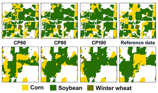
Figure 9 presents the classification results generated using the 9 by 9 training patch that produced a significant difference in the overall accuracy with respect to different class purity values. The classification results generated using other patch sizes and different class purity values in Illinois are presented in Figure S2. The distinctive differences between the classification results for different class purity values can be highlighted in two subareas, denoted as A and B in Figure 9. For CP 100, the exaggeration of soybean parcels and the misclassification of small corn parcels as soybean were observed. This occurred because the training patches selected primarily inside the crop parcels could not provide information regarding the discrimination of different crop types located at the boundary of the parcels. By contrast, the misclassification of corn parcels surrounded by the soybean parcels reduced significantly when using training patches with CP60. When a lower class purity value was applied to select the training patches, those located at the boundary between different crop parcels were primarily selected. Consequently, the 2D-CNN model trained using these training patches extracted spatial features that were useful to discriminate adjacent crops, thereby achieving increased classification accuracy. However, misclassified pixels were identified inside the crop parcels in subarea A of Figure 9, as observed for CP60 in Anbandegi, which is a limitation of using small training patches.
Table 6 summarizes the accuracy statistics of one classification result generated using a 9 by 9 patch shown in Figure 9. The accuracy statistics of the classification results using other patch sizes and different class purity values in Illinois are also listed in Table S2. As indicated in Figure 8, the overall accuracy for CP60 was higher than that for CP100. This improvement in overall accuracy was attributed to the significant increase of approximately 7.3%p in the producer’s accuracy of corn, which is one of the major crops in the Illinois region. In the case of CP100, the user’s accuracy of soybean decreased significantly by 4.4%p owing to the misclassification of corn as soybean, as shown in Figure 9.
The Illinois region exhibited lower GCH and higher CV values than the Anbandegi region, as shown in Figure 5. This implies the heterogeneous distributions of crop parcels and the large variations in class homogeneity within a patch across the study area. Consequently, using training patches with a low class purity value allows crops to be discriminated more accurately. Many training patches collected at the boundaries between crop parcels contributed to the correct identification of adjacent crop parcels. The significant decrease in classification accuracy when using large training patches was due to the inclusion of more subareas having non-uniform class homogeneity with a patch. Based on the results in the Illinois region, using training patches with low class purity and a smaller size is more likely to produce more accurate results in the classification of regions with heterogeneous crop distributions using mid-resolution remote sensing imagery.
4. Discussion
4.1. Novelty of the Study and Implications for Training Sample Selection
Previous studies for supervised classification emphasized the importance of collecting informative training samples and investigated the effects of different strategies in selecting training samples on classification performance [9,10,11,12,14,21]. However, the strategies on selecting informative training samples were developed for pixel-based classification. Because training patches that contain neighboring pixels are used in patch-based classification, classification performance is affected by both the representativeness of a training patch for a specific class and the degree of compositional homogeneity of classes within a training patch. These two factors are related to landscape heterogeneity of the study area [21,42,43]. Smith et al. [42,43] reported that classification accuracy decreased as land-cover heterogeneity increased and patch size decreased in USA. However, the evaluation was based on the comparison between classification accuracy and landscape variables, not on classification results. In patch-based classification, Sharma et al. [30] used training samples that have a class purity value of more than 60% for CNN-based classification without comparison with other class purity values. Song et al. [31] quantified the degree of class heterogeneity and then analyzed its effects on classification accuracy of patch-based CNN. An experiment on the classification of Landsat imagery revealed that moderately heterogeneous samples produced the highest accuracy. However, landscape heterogeneity was only used to demonstrate the superiority of patch-based CNN over pixel-based classifier, not to explicitly relate the global or local characteristics of landscape heterogeneity in the study area to classification performance.
In contrast to previous studies, the novelty of this study lies in the explicit quantification of the effect of class purity of a training patch on patch-based crop classification through comparative experiments conducted in two regions with different landscape characteristics and input images. Crop classification experiments demonstrated that the class purity within a training patch significantly affected the classification results, including the accuracy and spatial distributions because the information content provided by patch-based training samples varies according to the diversity of class composition in a patch. The relatively large crop parcel or the inside of the parcel (homogeneous subareas) was correctly classified using training patches with high class purity. By contrast, training patches with low class purity could discriminate both adjacent crops and the crop type near boundaries (heterogeneous subareas) more successfully. This effectiveness of training patches with low class purity for the heterogeneous distributions of land-cover class is similar to the results from previous pixel-based classification studies that emphasized the necessity of including training data that lie close to the location of boundaries in a geographic [9] or feature space [44]. This study also newly defined the GCH and CV of the LCH that can be useful quantitative measures for the GCH and degree of relative variations of class homogeneity across the study area, respectively. These quantitative indices were used for the characterization of class homogeneity of the study area and the interpretations of classification results. If such summary statistics in the study area can be combined with the LCH, it may be possible to pinpoint the locations of informative training samples that are specific to the discrimination of subareas with different local homogeneity.
It should be noted that class purity is inter-related to other factors, such as landscape heterogeneity, training patch size, and spatial resolution of input images. Chen et al. [22] reported that both sample impurity and landscape heterogeneity affect the classification accuracy in pixel-based classification with coarse resolution MODIS images. The sample impurity corresponded to class purity in this study, and the landscape heterogeneity was opposite to the GCH defined in this study. In particular, when the landscape heterogeneity was high, the corresponding classification accuracy decreased. The Illinois region classified in this study also exhibited high class heterogeneity. However, the classification accuracy was improved significantly when small size training patches with low class purity were used for classification. Therefore, training samples in patch-based classification should be collected by considering both characteristics of the study area (class purity and landscape homogeneity) and the classification parameter (patch size in CNN-based classification).
The spatial resolution of remote sensing images used for classification is also one of the important factors for the collection of training samples in supervised classification. Many studies have demonstrated that landscape heterogeneity and training sample size might vary according to the spatial resolution [21,39,45]. In this study, the LCH was defined to properly account for the difference in spatial resolution of input images in two classification regions (0.25 m vs. 30 m). The Pi value in Equation (1) can vary with respect to the spatial resolution of the input images. This indicates that the strategy for training sample collection based on class purity should be changed because LCH values may change accordingly even in the same region when remote sensing images with different spatial resolution are used. For example, when coarser spatial resolution images are used for classification in Anbandegi, the LCH values will decrease accordingly; hence, a different reference class purity value should be determined. Furthermore, the spatial resolution affects the quantity of the training patches. If a high class purity value is selected for the classification with coarse spatial resolution images, only a small number of training patches may be collected, similar to the Illinois case. Therefore, the class purity, LCH, and GCH defined in this study should be used to collect training patches according to the spatial resolution of the input images.
Deep learning-based classifiers require the sufficient amount of training samples to achieve satisfactory classification performance [28,29]. If such a small number of training patches are used for CNN-based classification, it may be difficult to seek the optimal parameters of deep neutral network structures, thereby yielding poor classification performance. In addition to the quantity of training samples, the quality of training samples is important in supervised classification because the learning process is based on the representativeness of the training samples for the classes of interest. In particular, the classification results of deep learning models depend on high-level features extracted from representation learning with training patches [46,47]. Therefore, the information content contained in training patches is critical for extracting informative spatial features. As discussed, using training patches with different class purity values and patch sizes produces spatial features with different characteristics. Hence, training patches with a specific class purity and patch size based on class homogeneity in the study area should be selected to discriminate homogeneous subareas (inside the parcels) from heterogeneous ones (boundaries between parcels) and vice versa.
4.2. Limitations and Future Research Directions
The major findings in this study can provide guidance for selecting training samples in patch-based classification; however, further investigation and confirmation are necessitated. In this study, crop type information from ground truth data was used to analyze the effects of class purity in a training patch and quantify the spatial homogeneity of the study area. From a practical viewpoint, however, such ground truth information is not always available, which renders it impossible to calculate the class purity and other quantitative indices. This limitation of the sampling strategy using class purity and quantitative indices presented herein may be relieved using a past land-cover map in the study area of interest. Unless significant changes have occurred in the study area, one can quantify the class homogeneity of the study area using land-cover types in a past land-cover map. This class homogeneity information can be used as a prior basis to determine the appropriate class purity and patch size values in the study area. However, more extensive experiments should be conducted to determine the appropriate reference or threshold value of class purity and the optimal patch size. In this study, the strategy for selecting training patches based on class purity is based fully on class-type information, but may not account for the spectral information of class type. The same class type may exhibit different spectral characteristics, and mixed pixel effects are also typical in classifications using coarse spatial resolution remote sensing images [13,14]. Hence, the effects of spectral purity should be analyzed via spectral unmixing [48,49] in conjunction with those of class purity of training patches in future work.
5. Conclusions
Previous studies have tested the effects of training samples on classification accuracy in supervised classification, but a comparative analysis of training sample selection considering variations of class purity within a training patch has not yet been fully performed in patch-based classification. This analysis is important in patch-based classification because classification accuracy is sensitive to the information content of training patches. In this study, the effects of class purity in a training patch on the performance of crop classification using a 2D-CNN were investigated through crop classification experiments conducted in two regions with different spatial homogeneity. Two quantitative measures were also used to quantify global class homogeneity of the study area and local variations of class homogeneity across the study area. Crop classification experiments conducted in two regions with different class compositions and spatial homogeneity demonstrated that the class purity of a training patch and patch size had significant influence on the classification accuracy, depending on the class homogeneity of the study area. For the classification of regions with high class homogeneity using high resolution remote sensing imagery, using large training patches with high class purity is beneficial. Meanwhile, small training patches with low class purity are effective for the classification of regions with high class heterogeneity using coarse resolution remote sensing imagery. These results indicate that the classification accuracy of patch-based classification can be improved using informative training samples selected by considering both class purity and spatial homogeneity of the study area. Therefore, the key findings of this study are expected to serve as a useful basis for selecting training samples in patch-based supervised classification; however, to expand the applicability of the major findings of this study, other important issues not investigated in this study, including consideration of spectral purity with class purity and selection of an appropriate threshold value of class purity, should be investigated through extensive experiments.
Supplementary Materials
The following are available online at https://www.mdpi.com/2076-3417/10/11/3773/s1, Figure S1: Classification results generated using other patch sizes and different class purity values in Anbandegi: (a) 5 by 5 patch; (b) 13 by 13 patch, (c) 15 by 15 patch; and (d) 21 by 21 patch. Each map is one of four classification results with the highest overall accuracy. Figure S2: Classification results generated using other patch sizes and different class purity values in Illinois: (a) 5 by 5 patch; (b) 9 by 9 patch; and (c) 15 by 15 patch. Each map is one of four classification results with the highest overall accuracy. Table S1: Accuracy statistics of the classification results using other patch sizes and different class purity values in Anbandegi (PA: producer’s accuracy; UA: user’s accuracy; OA: overall accuracy). Classification accuracy values from one of four classification results with the highest overall accuracy are displayed. Table S2: Accuracy statistics of the classification results using other patch sizes and different class purity values in Illinois (PA: producer’s accuracy; UA: user’s accuracy; OA: overall accuracy). Classification accuracy values from one of four classification results with the highest overall accuracy are displayed.
Author Contributions
Conceptualization, S.P. and N.-W.P.; methodology, S.P. and N.-W.P.; software, S.P.; validation, S.P.; formal analysis, S.P.; investigation, S.P. and N.-W.P.; writing—original draft preparation, S.P.; writing—review and editing, N.-W.P.; supervision, N.-W.P.; Funding acquisition, N.-W.P. All authors have read and agreed to the published version of the manuscript.
Funding
This work was supported by INHA UNIVERSITY Research Grant.
Acknowledgments
The authors thank Chan-Won Park, Kyung-Do Lee, Sang-Il Na, and Ho-Young Ahn from the National Institute of Agricultural Sciences for providing UAV imagery and ground truth data in the Anbandegi region. The authors also thank three anonymous reviewers for their constructive comments on the manuscript.
Conflicts of Interest
The authors declare no conflict of interest.
References
- Cheng, G.; Han, J.; Lu, X. Remote sensing image scene classification: Benchmark and state of the art. Proc. IEEE 2017, 105, 1865–1883. [Google Scholar] [CrossRef] [Green Version]
- Kwak, G.-H.; Park, S.; Yoo, H.Y.; Park, N.-W. Updating land cover maps using object segmentation and past land cover information. Korean J. Remote Sens. 2017, 33, 1089–1100, (In Korean with English Abstract). [Google Scholar]
- Na, S.-I.; Park, C.-W.; So, K.-H.; Ahn, H.-Y.; Lee, K.-D. Development of biomass evaluation model of winter crop using RGB imagery based on unmanned aerial vehicle. Korean J. Remote Sens. 2018, 34, 709–720, (In Korea with English Abstract). [Google Scholar]
- Lee, Y.-S.; Lee, S.; Jung, H.-S. Mapping forest vertical structure in Gong-ju, Korea using Sentinel-2 satellite images and artificial neural networks. Appl. Sci. 2020, 10, 1666. [Google Scholar] [CrossRef] [Green Version]
- Kim, Y.; Park, N.-W.; Lee, K.-D. Self-learning based land-cover classification using sequential class patterns from past land-cover maps. Remote Sens. 2017, 9, 921. [Google Scholar] [CrossRef] [Green Version]
- Zurqani, H.A.; Post, C.J.; Mikhailova, E.A.; Allen, J.S. Mapping urbanization trends in a forested landscape using Google Earth Engine. Remote Sens. Earth Syst. Sci. 2019, 2, 173–182. [Google Scholar] [CrossRef]
- Kwak, G.-H.; Park, N.-W. Impact of texture information on crop classification with machine learning and UAV images. Appl. Sci. 2019, 9, 643. [Google Scholar] [CrossRef] [Green Version]
- Belgiu, M.; Drǎguţ, L. Comparing supervised and unsupervised multiresolution segmentation approaches for extracting buildings from very high resolution imagery. ISPRS J. Photogramm. Remote Sens. 2014, 96, 67–75. [Google Scholar] [CrossRef] [Green Version]
- Foody, G.M.; Mathur, A. The use of small training sets containing mixed pixels for accurate hard image classification: Training on mixed spectral responses for classification by a SVM. Remote Sens. Environ. 2006, 103, 179–189. [Google Scholar]
- Mathur, A.; Foody, G.M. Crop classification by support vector machine with intelligently selected training data for an operational application. Int. J. Remote Sens. 2008, 29, 2227–2240. [Google Scholar]
- Shao, Y.; Lunetta, R.S. Comparison of support vector machine, neural network, and CART algorithms for the land-cover classification using limited training data points. ISPRS J. Photogramm. Remote Sens. 2012, 70, 78–87. [Google Scholar] [CrossRef]
- Millard, K.; Richardson, M. On the importance of training data sample selection in random forest image classification: A case study in peatland ecosystem mapping. Remote Sens. 2015, 7, 8489–8515. [Google Scholar] [CrossRef] [Green Version]
- Villa, A.; Chanussot, J.; Benediktsson, J.A.; Jutten, C. Spectral unmixing for the classification of hyperspectral images at a finer spatial resolution. IEEE J. Sel. Topics Signal Process. 2010, 5, 521–533. [Google Scholar] [CrossRef] [Green Version]
- Foody, G.M.; Arora, M.K. Incorporating mixed pixels in the training, allocation and testing stages of supervised classifications. Pattern Recog. Lett. 1996, 17, 1389–1398. [Google Scholar] [CrossRef]
- Brown, M.; Gunn, S.R.; Lewis, H.G. Support vector machines for optimal classification and spectral unmixing. Ecol. Model. 1999, 120, 167–179. [Google Scholar] [CrossRef]
- Mianji, F.A.; Zhang, Y. SVM-based unmixing-to-classification conversion for hyperspectral abundance quantification. IEEE Trans. Geosci. Remote Sens. 2011, 49, 4318–4327. [Google Scholar] [CrossRef]
- Zhang, B.; Sun, X.; Gao, L.; Yang, L. Endmember extraction of hyperspectral remote sensing images based on the ant colony optimization (ACO) algorithm. IEEE Trans. Geosci. Remote Sens. 2011, 49, 2635–2646. [Google Scholar] [CrossRef]
- Yang, C.; Wu, G.; Ding, K.; Shi, T.; Li, Q.; Wang, J. Improving land use/land cover classification by integrating pixel unmixing and decision tree methods. Remote Sens. 2017, 9, 1222. [Google Scholar] [CrossRef] [Green Version]
- Kavzoglu, T. Increasing the accuracy of neural network classification using refined training data. Environ. Model. Softw. 2009, 24, 850–858. [Google Scholar] [CrossRef]
- Ozdarici Ok, A.; Akyurek, Z. Automatic training site selection for agricultural crop classification: A case study on Karacabey plain, Turkey. Int. Arch. Photogramm. Remote Sens. Spat. Inf. Sci. 2011, 3819, 221–225. [Google Scholar] [CrossRef] [Green Version]
- Chen, D.; Stow, D. The effect of training strategies on supervised classification at different spatial resolutions. Photogramm. Eng. Remote Sens. 2002, 68, 1155–1162. [Google Scholar]
- Chen, Y.; Song, X.; Wang, S.; Huang, J.; Mansaray, L.R. Impacts of spatial heterogeneity on crop area mapping in Canada using MODIS data. ISPRS J. Photogramm. Remote Sens. 2016, 119, 451–461. [Google Scholar] [CrossRef]
- Zhang, L.; Zhang, L.; Du, B. Deep learning for remote sensing data: A technical tutorial on the state of the art. IEEE Geosci. Remote Sens. Mag. 2016, 4, 22–40. [Google Scholar] [CrossRef]
- Zhu, X.X.; Tuia, D.; Mou, L.; Xia, G.-S.; Zhang, L.; Xu, F.; Fraundorfer, F. Deep learning in remote sensing data: A comprehensive review and list of resources. IEEE Geosci. Remote Sens. Mag. 2017, 5, 8–36. [Google Scholar] [CrossRef] [Green Version]
- Maggiori, E.; Tarabalka, Y.; Charpiat, G.; Alliez, P. Convolutional neural networks for large-scale remote-sensing image classification. IEEE Trans. Geosci. Remote Sens. 2016, 55, 645–657. [Google Scholar] [CrossRef] [Green Version]
- Wang, Z.-Y.; Xia, Q.-M.; Yan, J.-W.; Xuan, S.-Q.; Su, J.-H.; Yang, C.-F. Hyperspectral image classification based on spectral and spatial information using multi-scale ResNet. Appl. Sci. 2019, 9, 4890. [Google Scholar] [CrossRef] [Green Version]
- Park, M.-G.; Kwak, G.-H.; Park, N.-W. A convolutional neural network model with weighted combination of multi-scale spatial features for crop classification. Korean J. Remote Sens. 2019, 35, 1273–1283, (In Korean with English Abstract). [Google Scholar]
- Li, Y.; Zhang, H.; Shen, Q. Spectral–spatial classification of hyperspectral imagery with 3D convolutional neural network. Remote Sens. 2017, 9, 67. [Google Scholar] [CrossRef] [Green Version]
- Kim, Y.; Kwak, G.-H.; Lee, K.-D.; Na, S.-I.; Park, C.-W.; Park, N.-W. Performance evaluation of machine learning and deep learning algorithms in crop classification: Impact of hyper-parameters and training sample size. Korean J. Remote Sens. 2018, 34, 811–827, (In Korean with English Abstract). [Google Scholar]
- Sharma, A.; Liu, X.; Yang, X.; Shi, D. A patch-based convolutional neural network for remote sensing image classification. Neural Netw. 2017, 95, 19–28. [Google Scholar]
- Song, H.; Kim, Y.; Kim, Y. A patch-based light convolutional neural network for land-cover mapping using Landsat-8 images. Remote Sens. 2019, 11, 114. [Google Scholar]
- Kwak, G.-H.; Park, M.-G.; Park, C.-W.; Lee, K.-D.; Na, S.-I.; Ahn, H.-Y.; Park, N.-W. Combining 2D CNN and bidirectional LSTM to consider spatio-temporal features in crop classification. Korean J. Remote Sens. 2019, 35, 681–692, (In Korean with English Abstract). [Google Scholar]
- Muñoz-Marí, J.; Bruzzone, L.; Camps-Valls, G. A support vector domain description approach to supervised classification of remote sensing images. IEEE Trans. Geosci. Remote Sens. 2007, 45, 2683–2692. [Google Scholar] [CrossRef]
- Zhu, Z.; Gallant, A.L.; Woodcock, C.E.; Pengra, B.; Olofsson, P.; Loveland, T.R.; Jin, S.; Dahal, D.; Yang, L.; Auch, R.F. Optimizing selection of training and auxiliary data for operational land cover classification for the LCMAP initiative. ISPRS J. Photogramm. Remote Sens. 2016, 122, 206–221. [Google Scholar] [CrossRef] [Green Version]
- Cracknell, M.J.; Reading, A.M. Geological mapping using remote sensing data: A comparison of five machine learning algorithms, their response to variations in the spatial distribution of training data and the use of explicit spatial information. Comput. Geosci. 2014, 63, 22–33. [Google Scholar] [CrossRef] [Green Version]
- Environmental Geographic Information Service (EGIS). Available online: http://egis.me.go.kr (accessed on 1 August 2019).
- USGS Global Visualization Viewer (GloVis). Available online: https://glovis.usgs.gov (accessed on 12 August 2019).
- CropScape. Available online: https://nassgeodata.gmu.edu/CropScape (accessed on 12 August 2019).
- Löw, F.; Duveiller, G. Defining the spatial resolution requirements for crop identification using optical remote sensing. Remote Sens. 2014, 6, 9034–9063. [Google Scholar]
- Ji, S.; Zhang, C.; Xu, A.; Shi, Y.; Duan, Y. 3D convolutional neural network for crop classification with multi-temporal remote sensing images. Remote Sens. 2018, 10, 75. [Google Scholar] [CrossRef] [Green Version]
- Lillesand, T.M.; Kiefer, R.W.; Chipman, J.W. Remote Sensing and Image Interpretation, 6th ed.; Wiley: Hoboken, NJ, USA, 2008; pp. 585–586. [Google Scholar]
- Smith, J.H.; Wickham, J.D.; Stehman, S.V.; Yang, L. Impacts of patch size and land-cover heterogeneity on thematic image classification accuracy. Photogramm. Eng. Remote Sens. 2002, 68, 65–70. [Google Scholar]
- Smith, J.H.; Stehman, S.V.; Wickham, J.D.; Yang, L. Effects of landscape characteristics on land-cover class accuracy. Remote Sens. Environ. 2003, 84, 342–349. [Google Scholar] [CrossRef]
- Foody, G.M. The significance of border training patterns in classification by a feedforward neural network using back propagation learning. Int. J. Remote Sens. 1999, 20, 3549–3562. [Google Scholar] [CrossRef]
- Liu, J.; Liu, H.; Heiskanen, J.; Mõttus, M.; Pellikka, P. Posterior probability-based optimization of texture window size for image classification. Remote Sens. Lett. 2014, 5, 753–762. [Google Scholar] [CrossRef]
- Scott, G.J.; England, M.R.; Starms, W.A.; Marcum, R.A.; Davis, C.H. Training deep convolutional neural networks for land-cover classification of high-resolution imagery. IEEE Geosci. Remote Sens. Lett. 2017, 14, 549–553. [Google Scholar] [CrossRef]
- Bradley, P.E.; Keller, S.; Weinmann, M. Unsupervised feature selection based on ultrametricity and sparse training data: A case study for the classification of high-dimensional hyperspectral data. Remote Sens. 2018, 10, 1564. [Google Scholar] [CrossRef] [Green Version]
- Adams, J.B.; Sabol, D.E.; Kapos, V.; Filho, R.A.; Roberts, D.A.; Smith, M.O.; Gillespie, A.R. Classification of multispectral images based on fractions of endmembers: Application to land-cover change in the Brazilian Amazon. Remote Sens. Environ. 1995, 52, 137–154. [Google Scholar]
- Zhao, J.; Zhong, Y.; Hu, X.; Wei, L.; Zhang, L. A robust spectral-spatial approach to identifying heterogeneous crops using remote sensing imagery with high spectral and spatial resolutions. Remote Sens. Environ. 2020, 239, 111605. [Google Scholar] [CrossRef]
Figure 1.
Datasets used for crop classification in Anbandegi: (a) true color unmanned aerial vehicle (UAV) imagery; (b) ground truth map; and (c) field photos.
Figure 1.
Datasets used for crop classification in Anbandegi: (a) true color unmanned aerial vehicle (UAV) imagery; (b) ground truth map; and (c) field photos.

Figure 2.
Data sets used for crop classification in Illinois: (a) false color composite (near-infrared (NIR)–short-wave infrared (SWIR)–Red) of Landsat-8 Operational Land Imager (OLI) imagery on 8 April 2017; (b) cropland data layers (CDL) data.
Figure 2.
Data sets used for crop classification in Illinois: (a) false color composite (near-infrared (NIR)–short-wave infrared (SWIR)–Red) of Landsat-8 Operational Land Imager (OLI) imagery on 8 April 2017; (b) cropland data layers (CDL) data.

Figure 3.
Examples of a 5 by 5 training patch candidate with different class compositions and configurations; (a) a case that can be a training patch for class A with a class purity value of 60%; (b) cases that cannot be a training patch for class A. The box with thick lines denotes a center pixel of a training patch. Different colors refer to different classes.

Figure 4.
Flow chart of selection of training patch candidates with respect to class purity and patch size.
Figure 4.
Flow chart of selection of training patch candidates with respect to class purity and patch size.

Figure 5.
Variation in (a) global class homogeneity (GCH) and (b) coefficient of variation of class homogeneity (CV) of two study regions.
Figure 5.
Variation in (a) global class homogeneity (GCH) and (b) coefficient of variation of class homogeneity (CV) of two study regions.

Figure 6.
Variations in overall accuracy with respect to five different patch sizes for different class purity values in Anbandegi.
Figure 6.
Variations in overall accuracy with respect to five different patch sizes for different class purity values in Anbandegi.

Figure 7.
Classification results with respect to different class purity values when using a 9 by 9 patch in Anbandegi.
Figure 7.
Classification results with respect to different class purity values when using a 9 by 9 patch in Anbandegi.

Figure 8.
Variations in overall accuracy with respect to three different patch sizes for different class purity values in Illinois.
Figure 8.
Variations in overall accuracy with respect to three different patch sizes for different class purity values in Illinois.

Figure 9.
Classification results with respect to different class purity values when using a 9 by 9 patch in Illinois. Two subareas denoted as A and B are zoomed out for comparison purposes.
Figure 9.
Classification results with respect to different class purity values when using a 9 by 9 patch in Illinois. Two subareas denoted as A and B are zoomed out for comparison purposes.


Table 1.
Summary of UAV imagery used for crop classification in Anbandegi.
| Category | Specification |
|---|---|
| UAV model | eBee Classic |
| Camera | Canon IXUS/ELPH |
| Image size | 2629 by 3275 |
| Area of crop parcels | 28.7 ha |
| Spectral bands | Blue, Green, Red |
| Spatial resolution | 0.25 m |
| Acquisition date | 25 August 2017 |
Table 2.
Summary of Landsat-8 OLI images used for crop classification in Illinois.
| Category | Specification |
|---|---|
| Satellite/Sensor | Landsat-8 OLI |
| Image size | 633 by 673 |
| Area of crop parcels | 198,476 ha |
| Spectral bands | Red, NIR, SWIR |
| Spatial resolution | 30 m |
| Acquisition date | 7 March 2017 |
| 8 April 2017 | |
| 27 May 2017 | |
| 15 September 2017 | |
| 17 October 2017 |
Table 3.
Two-dimensional convolutional neural network (2D-CNN) architecture applied in this study. P and F refer to the patch size and number of filters, respectively.
Table 3.
Two-dimensional convolutional neural network (2D-CNN) architecture applied in this study. P and F refer to the patch size and number of filters, respectively.
| Layer Type/Method | Output Dimension | Number of Parameters |
|---|---|---|
| Conv2D_1 | (P, P, F) | 896 |
| Conv2D_2 | (P, P, F) | 9248 |
| Max-pooling2D | (P/2, P/2, F) | 0 |
| Conv2D_3 | (P/2, P/2, F × 2) | 18,496 |
| Dropout | 256 neurons | 0 |
| Flattening | 256 neurons | 0 |
| ReLu | 64 neurons | 16,448 |
| Softmax | 4 neurons | 260 |
Table 4.
List of hyper-parameters of 2D-CNN models applied to the two study areas.
| Classifier | Parameters | Value | |
|---|---|---|---|
| Anbandegi | Illinois | ||
| 2D-CNN | Dropout rate | 0.2 | |
| Patch size | 5, 9, 13, 17, 21 | 5, 9, 15 | |
| Kernel size | 3 | ||
| Number of filters | 32 | ||
Table 5.
Accuracy statistics with respect to different class purity values when using a 9 by 9 patch in Anbandegi (PA: producer’s accuracy; UA: user’s accuracy; OA: overall accuracy).
Table 5.
Accuracy statistics with respect to different class purity values when using a 9 by 9 patch in Anbandegi (PA: producer’s accuracy; UA: user’s accuracy; OA: overall accuracy).
| CP60 | CP80 | CP100 | ||||
|---|---|---|---|---|---|---|
| PA (%) | UA (%) | PA (%) | UA (%) | PA (%) | UA (%) | |
| Highland Kimchi cabbage | 94.79 | 82.70 | 95.08 | 87.71 | 93.12 | 88.91 |
| Cabbage | 72.16 | 87.52 | 71.89 | 92.40 | 72.66 | 94.85 |
| Potato | 90.12 | 84.96 | 95.12 | 74.02 | 96.57 | 77.75 |
| Fallow | 49.50 | 79.62 | 58.00 | 79.59 | 73.55 | 74.82 |
| OA (%) | 83.78 | 85.49 | 86.56 | |||
Table 6.
Accuracy statistics with respect to different class purity values when using a 9 by 9 patch in Illinois (PA: producer’s accuracy; UA: user’s accuracy; OA: overall accuracy).
Table 6.
Accuracy statistics with respect to different class purity values when using a 9 by 9 patch in Illinois (PA: producer’s accuracy; UA: user’s accuracy; OA: overall accuracy).
| CP60 | CP80 | CP100 | ||||
|---|---|---|---|---|---|---|
| PA (%) | UA (%) | PA (%) | UA (%) | PA (%) | UA (%) | |
| Corn | 82.13 | 73.76 | 80.61 | 73.22 | 74.83 | 72.00 |
| Soybean | 76.87 | 86.76 | 77.42 | 86.11 | 75.96 | 82.32 |
| Winter wheat | 95.06 | 83.96 | 90.09 | 80.76 | 90.86 | 77.56 |
| OA (%) | 81.43 | 80.44 | 77.87 | |||
© 2020 by the authors. Licensee MDPI, Basel, Switzerland. This article is an open access article distributed under the terms and conditions of the Creative Commons Attribution (CC BY) license (http://creativecommons.org/licenses/by/4.0/).
Share and Cite
MDPI and ACS Style
Park, S.; Park, N.-W. Effects of Class Purity of Training Patch on Classification Performance of Crop Classification with Convolutional Neural Network. Appl. Sci. 2020, 10, 3773. https://doi.org/10.3390/app10113773
AMA Style
Park S, Park N-W. Effects of Class Purity of Training Patch on Classification Performance of Crop Classification with Convolutional Neural Network. Applied Sciences. 2020; 10(11):3773. https://doi.org/10.3390/app10113773
Chicago/Turabian StylePark, Soyeon, and No-Wook Park. 2020. "Effects of Class Purity of Training Patch on Classification Performance of Crop Classification with Convolutional Neural Network" Applied Sciences 10, no. 11: 3773. https://doi.org/10.3390/app10113773
Note that from the first issue of 2016, this journal uses article numbers instead of page numbers. See further details here.