Contactless Localization of Premature Laminar–Turbulent Flow Transitions on Wind Turbine Rotor Blades in Operation


Automation and Quality Science, Bremen Institute for Metrology, University of Bremen, Linzer Str. 13, 28359 Bremen, Germany
*
Author to whom correspondence should be addressed.
Appl. Sci. 2020, 10(18), 6552; https://doi.org/10.3390/app10186552
Submission received: 27 August 2020
/
Revised: 15 September 2020
/
Accepted: 16 September 2020
/
Published: 19 September 2020
(This article belongs to the Collection Wind Energy: Current Challenges and Future Perspectives)
Abstract
:Featured Application
The evaluation of reduced laminar flow in the boundary layer of wind turbine rotor blades in operation introduced in this work enables estimations of wind turbine efficiency loss due to negative influence on the aerodynamic properties. This leads to a more efficient identification of maintenance and repair requirements.
Abstract
Thermographic flow visualization enables a noninvasive detection of the laminar–turbulent flow transition and allows a measurement of the impact of surface erosion and contamination due to insects, rain, dust, or hail by quantifying the amount of laminar flow reduction. The state-of-the-art image processing is designed to localize the natural flow transition as occurring on an undisturbed blade surface by use of a one-dimensional gradient evaluation. However, the occurrence of premature flow transitions leads to a high measurement uncertainty of the localized transition line or to a completely missed flow transition detection. For this reason, regions with turbulent flow are incorrectly assigned to the laminar flow region, which leads to a systematic deviation in the subsequent quantification of the spatial distribution of the boundary layer flow regimes. Therefore, a novel image processing method for the localization of the laminar–turbulent flow transition is introduced, which provides a reduced measurement uncertainty for sections with premature flow transitions. By the use of a two-dimensional image evaluation, local maximal temperature gradients are identified in order to locate the flow transition with a reduced uncertainty compared to the state-of-the-art method. The transition position can be used to quantify the reduction of the laminar flow regime surface area due to occurrences of premature flow transitions in order to measure the influence of surface contamination on the boundary layer flow. The image processing is applied to the thermographic measurement on a wind turbine of the type GE 1.5 sl in operation. In 11 blade segments with occurring premature flow transitions and a high enough contrast of the developed turbulence wedge, the introduced evaluation was able to locate the flow transition line correctly. The laminar flow reduction based on the evaluated flow transition position located with a significantly reduced systematic deviation amounts to for the given measurement and can be used to estimate the reduction of the aerodynamic lift. Therefore, the image processing method introduced allows a more accurate estimation of the effects of real environmental conditions on the efficiency of wind turbines in operation.
1. Introduction
1.1. Motivation
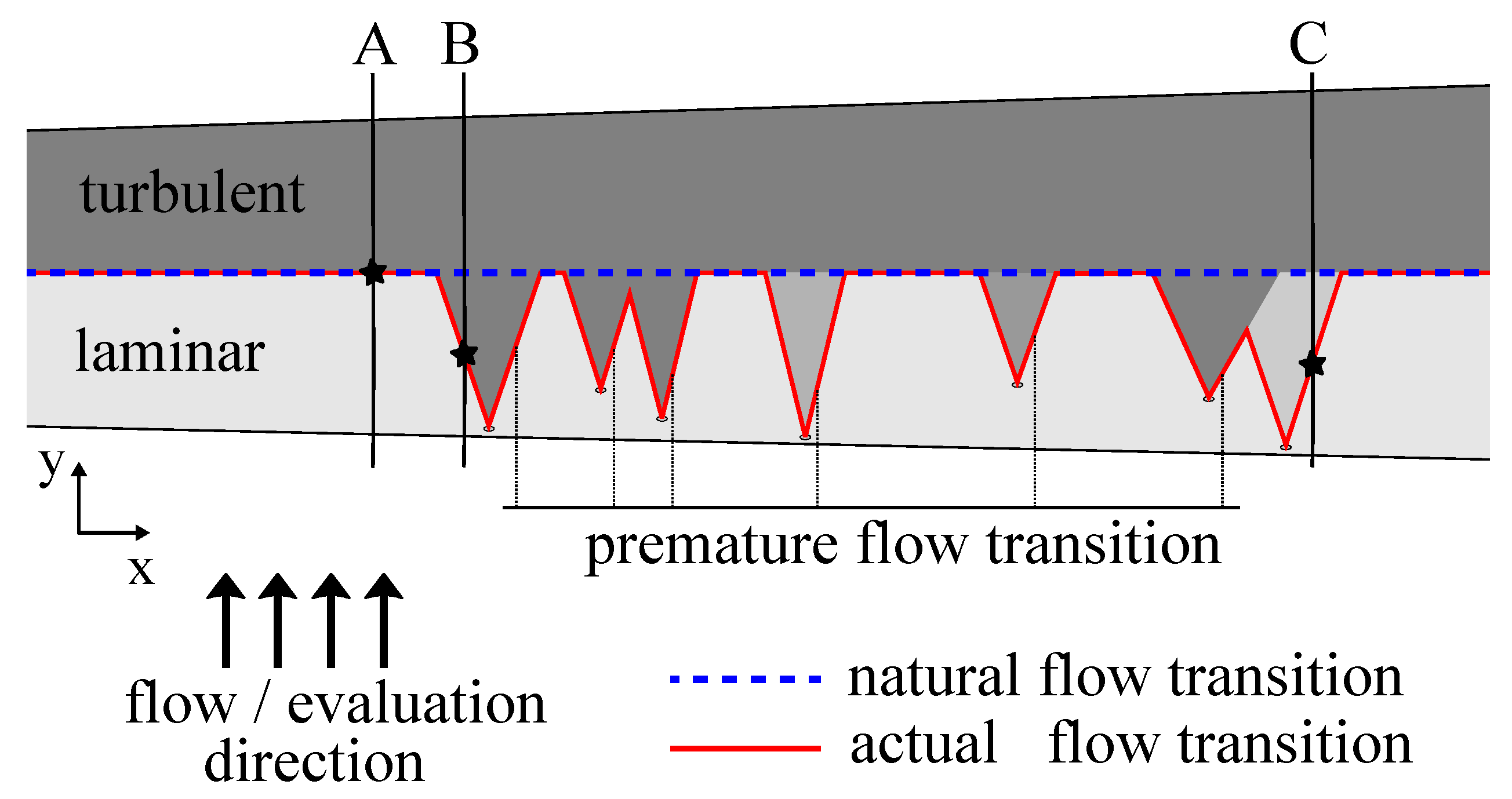
Disturbances of the surface on aerodynamic profiles have a significant impact on the boundary layer flow and, thus, the aerodynamic properties [1]. This is crucial for rotor blades of wind turbines as they are subject of contamination and erosion by insects [2], rain, dust, or hail [3,4,5] due to the environmental conditions and long-term operation. The adhesion of insects (contamination) and the surface damaging by impacting particles (erosion) changes the surface roughness of the leading edge of the rotor blades and triggers a premature laminar–turbulent flow transition [6] as well as a lengthening of the transition process [7] in the boundary layer. Such premature flow transitions develop a wedge-shaped area of turbulent flow (turbulence wedge) behind the surface defect that would otherwise be laminar, if the surface would be free of any disturbances, see Figure 1 [8,9]. This reduction of the overall size of the surface region with laminar flow causes a reduction in lift and increase in drag, which reduces the efficiency of a rotor blade, and thus the performance of the entire wind turbine [10,11].
Without a flow visualization on real wind turbines in operation and a subsequent mapping of the image plane onto the blade geometry, estimations of the reduction of the annual energy production due to surface disturbances leading to premature flow transitions can only be made with simulations or measurements on wind tunnel models by tripping the boundary layer flow intentionally with zig-zag tape [12]. The conditions in these experiments are idealized and resulting flow regimes arise from a binary solution of the surface disturbance [13]. Therefore, a measurement of the actual boundary layer flow influenced by surface disturbances on real wind turbines in operation is necessary. By locating the premature flow transitions, the actual position of the flow transition line can be used in blade-element-momentum simulations in order to estimate the reduction of the annual energy production.
1.2. State of the Art
Conventional flow visualization methods used on wind turbines like pressure measurements [14], oil flow [15], or tuft [16] visualization cannot be used for an evaluation of the boundary layer flow because the pressure taps, oil film, or tufts act as artificial surface disturbances itself. A contactless measurement technique without the need of a surface preparation enabling a noninvasive flow measurement is thermographic flow visualization [17,18,19]. This measurement technique is already in use for a variety of applications in wind tunnel experiments for detecting the laminar–turbulent transition or flow separation [20,21,22,23]. More recent studies begin to use thermography for analyzing surface defects on models of aerodynamic profiles [24,25].
A transfer of the thermographic flow visualization from wind tunnel experiments to field measurement applications on wind turbines in operation was recently introduced by Dollinger et al. [26,27]. However, the state-of-the-art image processing method for evaluating the thermographic images is optimized for locating the flow transition occurring naturally without any premature transitions triggered by surface disturbances. For retrieving the flow transition position on the rotor blade surface, the image processing method conducts temperature profile evaluations of one-pixel-wide lines in the thermographic image parallel to the flow direction and, thus, almost perpendicular to the leading edge [9], see for instance the vertical lines in Figure 1 for the cases A, B, and C. The position of the flow transition in each line is then determined by locating the maximum temperature gradient, as the transition between the laminar and turbulent flow regime creates a significant temperature step in flow direction. This image processing method was designed to evaluate the maximal temperature gradient for a flow transition perpendicular to the flow direction and evaluation line, because it minimizes the measurement uncertainty [28] and is subsequently referred to as the state-of-the-art method. A local surface disturbance, however, triggers a premature flow transition and creates a so-called turbulence wedge, see Figure 1. The flow transition along the flanks of the turbulence wedges is no longer perpendicular to the evaluation lines. In combination with an elongated transition process [7] due to the forced transition, the temperature step between the flow regimes is flattened in the evaluated temperature profile.
To illustrate this finding, the temperature profile and temperature gradient in y-direction are compared in Figure 2a,b, respectively. Both are shown for an example of no premature flow transition (A) and an example with premature flow transition (B) with a star symbol showing the actual flow transition position for both cases. While the temperature gradient forms a spike at the position of the temperature gradient maxima in case A, the maximum gradient for case B is surrounded by a constant gradient level. Therefore, a localization of the gradient maxima in case B has a lower sensibility compared to the maxima in case A. As a result, the uncertainty of the flow transition localization in sections with a surface disturbance, hence a premature flow transition (case B), is increased. Additionally, a weaker surface contamination such as an insect that is almost washed of by rain or a tiny surface defect can create a softer turbulence wedge with an intensity almost equal to the surrounding laminar flow regime, see the most right turbulence wedge in Figure 1. Even though the actual flow transition happens prematurely, the strongest temperature step still exists at the position where the flow transition would occur without a surface disturbance, see example gradient profile C in Figure 2. An evaluation of the maximum temperature gradient thus fails to detect a premature flow transition. As a result, the current thermographic image processing for studying premature flow transitions and the resulting laminar flow reduction suffers from an increased localization uncertainty and non-detections of premature flow transitions.
1.3. Aim and Outline
For this reason, an enhanced image processing method is introduced that improves the sensitivity for detecting and localizing premature flow transitions. The image processing is based on the a priori knowledge about the wedge shapes of the premature flow transitions and the temperature gradient evaluation over both image dimensions. As a consequence of the improved subdivision of the laminar and turbulent flow regime areas, the enhanced flow transition localization enables to quantify the laminar flow reduction (LFR) with an increased accuracy.
A description of the image processing for flow transition localization in thermographic images is given in Section 2, followed by the definition of the LFR as a figure of merit for the impact of surface disturbances on the boundary layer flow. In Section 3, the implementation of the image processing and the experimental setup of a field measurement on a wind turbine in operation for the thermographic flow visualization process is described. A simulated and measured thermographic image from a 1.5 MW wind turbine are used to verify and validate, respectively, the capabilities of the introduced image processing regarding the accurate flow transition localization and the determination of the LFR in the presence of premature transitions in Section 4. The article finishes with a conclusion and outlook in Section 5.
2. Measurement Approach
In order to quantify the influence on the boundary layer flow due to surface disturbances, the measurement approach can be divided into locating the position of the actual flow transition line (Section 2.1) and the natural flow transition line (Section 2.2). Both information are subsequently used to quantify the laminar flow reduction (Section 2.3).
2.1. Actual Flow Transition
As a first step, the actual transition between the laminar and turbulent flow regime on wind turbine rotor blades is located by identifying and locating local temperature gradient maxima in the thermographic image. Assuming the flow direction in the thermographic image is parallel to the y-axis as in Figure 1, one position of the actual flow transition is obtained from the located local temperature gradients maxima for each image column over the x-axis.
According to the simplified illustration in Figure 1, the actual flow transition line over the rotor blade can be divided in linear segments with three different orientations: One orientation follows the course of the natural flow transition (almost parallel to the leading edge) and one orientation each for the two flanks of the turbulence wedges where premature flow transitions occur. An analysis of multiple thermographic measurements shows that the two angles of the flanks of the turbulence wedges with respect to the y-axis are independent of the size or contrast of the individual wedges. Two different gradient evaluation methods are proposed and subsequently studied that use this a priori knowledge to locate the local temperature gradient maxima, representing the actual flow transition, with maximal sensitivity.
2.1.1. Method A: No Image Rotation and 2D Gradient Evaluation
For each image pixel, the temperature gradient components along the x- and y-axis in the image plane are calculated using a gradient image filter. Next, the gradient components are converted to polar coordinates so that the magnitude and direction of each gradient is obtained. A selection is then made of those gradients whose direction aligns perpendicular to one of the three orientations of the transition line segments. The selected gradients are sorted out again according to their magnitude by applying a minimum threshold. Using a small threshold when selecting the local gradients representing the premature flow transitions allows the detection of weak, low contrast turbulence wedges. A high threshold for the selection of gradients representing the natural flow transition on the other hand allows a robust detection of the natural flow transition in image columns without premature flow transitions. The result is a gradient image containing only those gradients that represent the flow transition line, which is denoted as the actual flow transition.
2.1.2. Method B: Image Rotation and 1D Gradient Evaluation
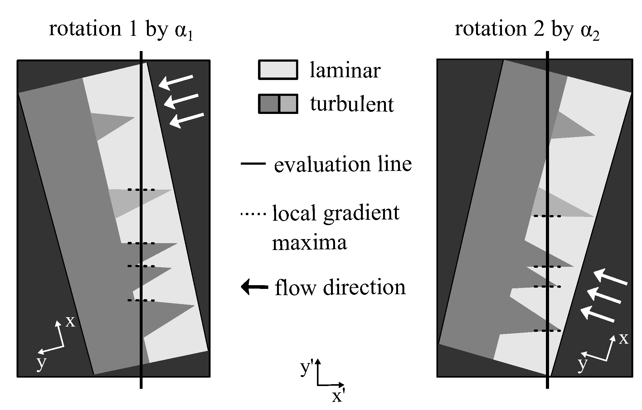
A more direct use of the a priori knowledge is achieved by an image rotation for each known transition line orientation in combination with a 1D gradient evaluation. The image is rotated to obtain directions of the 1D gradient evaluation perpendicular to one transition line segment, which provides maximal sensitivity and thus minimal uncertainty for localizing the position of the local temperature gradient maxima. Therefore, the original image is rotated three times to align each transition line segment parallel to the axis of the rotated image, see Figure 3. After each rotation, the gradient component parallel to the -axis is calculated for each image column (-position) and the local maxima are identified. The results are the positions of local gradient maxima in the three images for the three known orientations of the different transition line segments. Using different thresholds allows for a detection of weak, low-contrast turbulence wedges with small gradients representing the premature flow transitions (low threshold) and a robust natural flow transitions detection in image columns without any premature flow transition (higher threshold). After image re-rotation and combination of the results in a single image, the actual flow transition line is finally obtained.
2.2. Natural Flow Transition
Besides the premature flow transitions, the actual flow transition positions include the occurrences of the natural flow transitions in surface regions without premature flow transitions. In those regions, the transition forms a straight line and is almost parallel to the leading edge. For this reason, the natural flow transition is obtained from the actual flow transition positions by using an iterative linear regression algorithm, which is robust towards the premature flow transitions. A random subset of the positions is picked from which the initial regression line is calculated. Based on their distances to the regression line, the positions are included or excluded in the recalculation of the regression line. This iterative process is continued until the cumulative distance error of all included positions and the calculated line is below a certain threshold. The algorithm afterwards terminates and the final regression line is returned as the positions of the natural flow transition over the image columns .
2.3. Parameter Definition to Quantify the Laminar Flow Reduction (LFR)
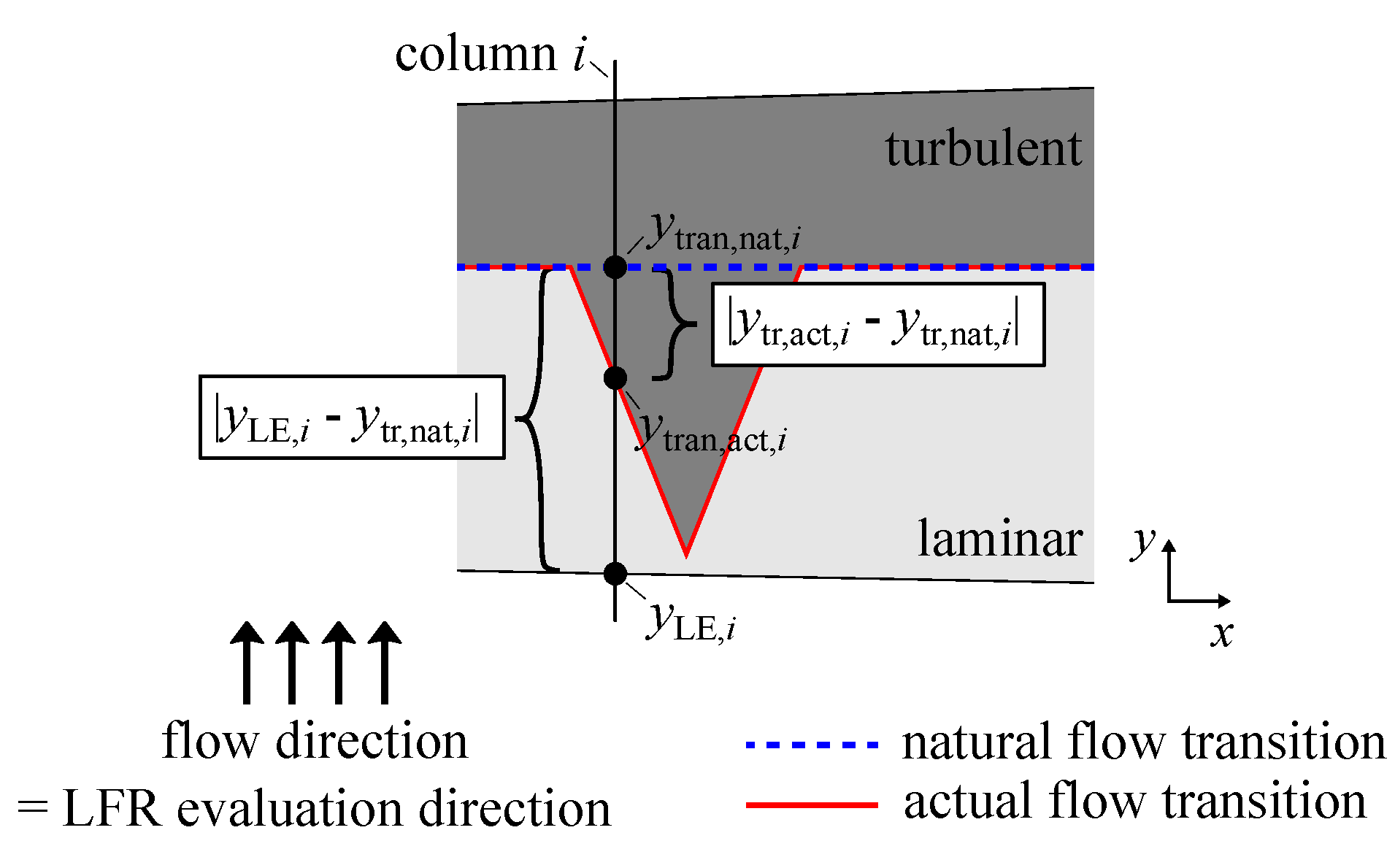
To evaluate the influence of premature flow transitions, the absolute distance between the natural transition and the actual transition in each image column i is calculated, see Figure 4. Divided by the absolute distance between the leading edge and the natural transition of the respective column, this yields the parameter
which quantifies the reduction of the laminar flow in the column i relative to the case of no premature flow transition. If the position of the actual flow transition equals the position of the natural flow transition, which means no premature transitions occur, equals 0. For a premature flow transition occurring near the leading edge, converges to 1.
To quantify the average LFR along the rotor blade or the image field of view, respectively, the average value of the laminar flow reduction over I image columns is considered:
3. Experimental Setup
The thermographic image in this work is conducted on a 1.5 MW horizontal wind turbine of the type GE 1.5 sl from the manufacturer General Electric. It has a hub height of 62 and a rotor diameter of 77 . Each of the three rotor blades have a length of . A photo of a typical measurement set-up is shown in Figure 5.
In the following the image acquisition for the thermographic flow visualization (Section 3.1) as well as the implemented image processing method for localizing the laminar–turbulent flow transitions (Section 3.2) is presented.
3.1. Image Acquisition
The thermographic image is conducted with a mobile system for free-field measurements on wind turbines in operation and consists of an infrared camera of the type imageIR 8300 from the manufacturer InfraTec. The actively cooled camera has a global shutter (snap-shot detector) and an InSb focal plane array with a format of 640 px × 512 px with a pixel size of 15 . The wavelength spectrum of the thermographic camera is sensitive between 2 –5 , and the noise equivalent temperature difference (NETD) is less than 25 at 30 . The dynamic range is 14 bit and the integration time is set to .
In order to maximize the spatial resolution of the thermographic images for the typical measurement distance between 100 –300 a 200 telelens optic is used. The lens has an angular aperture of 2.7° × 2.2° and with the given detector size the instantaneous field of view (IFOV) results in . For the typical measurement distance this results in a spatial resolution between 8.8–20 mm. The field of view along the longer axis with 640 px is between 5 and 14 m.
Due to the length of the rotor blade being more than twice the length of the maximum field of view of one image, the blade surface has to be captured in segments. Therefore, the IR-camera is triggered by an external optical system that signals the infrared camera the moment in which the rotor blade has a horizontal position parallel to the ground, resulting in an image acquisition of each rotor segment at the time of the same rotor blade orientation.
3.2. Implementation
The image processing for locating the flow transition is implemented in the script language Python. The algorithm is divided in four sub-routines which are listed and explained in detail below. A flow chart of the image processing is depicted in Figure 6.
- Pre-evaluation of the thermographic image
- Obtaining all local gradient maxima positions representing the natural and premature flow transition
- Selection of all gradient maxima with plausibility and outliers analysis
- Creating a final actual and natural flow transition line from the selected gradient maxima
- Calculation of the laminar flow reduction (LFR)
- 1.
- Pre-Evaluation
The first step is the deletion of outliers in the thermographic image due to pixel errors on the camera chip with the Navier–Stokes image inpainting method of the python library openCV [29] with a convergence interval of around the mean temperature. Afterwards, the image is normalized to an 8 bit intensity value range between 0 and 255. In order to spatially limit the subsequent evaluation steps, the image area representing the rotor blade surface is separated from the background by column-wisely locating the two absolute maximum temperature gradients. The locations of these gradient maxima are saved as the position of the rotor blade’s leading and trailing edge in the respective image column. All following evaluations steps are carried out within these borders.
- 2.
- Obtaining Positions of Local Gradient Maxima
The second sub-routine determines the positions of the local gradient maxima which meet the criteria of having a specific minimum magnitude above a given threshold and a specific direction corresponding to the known orientation of the flow transition segments. In order to achieve this, the two measurement approaches introduced in Section 2 are implemented.
3.2.1. Method A: No Image Rotation and 2D Gradient Evaluation
For the gradient evaluation method A, the Canny Edge algorithm of the openCV library is used. The algorithm first reduces noise with a 5 × 5 Gaussian filter with px before obtaining the first derivative in the horizontal and in the vertical direction with a 3 × 3 Sobel kernel. Afterwards, the gradients’ magnitude G and direction are calculated by
and
In order to thin out the detected edges in the image, a non-maximum suppression is conducted: The gradients of the neighboring pixel before and after the currently observed pixel in the direction of its gradient are investigated. If the current pixel represents the local maxima of these gradients, it is considered further, otherwise, it is suppressed. The last step applies a threshold test. All local gradients with a magnitude below a threshold are suppressed. Afterwards, a selection of the gradients on the basis of their direction corresponding to the a priori knowledge about the direction of the transition line segments is made.
In order to be sensitive with respect to weak, low-contrast turbulence wedges (case C of Section 1.2), a low threshold is chosen for the evaluation of the local gradient maxima that have a direction corresponding to the orientation of the premature flow transitions segments. For the evaluation of the gradients in direction of the flow, a higher threshold is used to robustly detected the local gradient maxima representing the natural flow transition as their magnitude is higher compared to premature flow transitions’ ones.
3.2.2. Method B: Image Rotation and 1D Gradient Evaluation
For the gradient evaluation method B, the thermographic image is rotated around the three rotation angles , , and , see Figure 3, each time aligning another group of transition segments parallel to the -axis of the rotated image and hence perpendicular to the vertical -axis. By conducting a subsequent column-wise gradient evaluation of the px Gauss-filtered temperature profiles for the columns of the rotated image, the position of all local gradient maxima above the threshold are saved. Because of the perpendicular alignment between the evaluation line and the respective transition segments, the local temperature gradients at the positions of the flow transition are maximized. The evaluation of all columns yields the collection of all local gradient maxima of the rotated image below the threshold. The gradient threshold used for the rotation angle is higher than for the other rotation angles and . This achieves a more robust detection of the natural flow transitions in the columns without a premature transition as the natural flow transition tends to develop a higher temperature gradient. The lower threshold for the two rotation angles and , on the other hand, preserves a higher sensitivity towards low gradients that can develop due to the premature flow transitions of low-contrast turbulence wedges. Combining all gradients of the and rotation yields all local gradient maxima positions representing the premature flow transitions. The local gradient maxima positions representing the natural flow transition which are obtained by the rotation angle are further noted as .
- 3.
- Selection of Local Gradient Maxima
After retrieving the local gradient maxima positions and , the first step is an approximation of the natural flow transition by evaluating . The robust linear RANSAC regression algorithm of the sklearn library is used as it excluded individual outliers. The result is the approximated linear course of the natural flow transition , which would be the flow transition if no premature transitions would exist. This approximation can be used in the following filtering steps. First, all columns with an entry in , which are near the approximated natural flow transition line, are set to the line’s column value, respectively, deleting the outliers. Additionally, the amount of pixels of each image column represented in is limited to one. Afterwards, holes of individual columns without a representative in are filled if surrounded by columns that are included in . The next step is to further select positions from by defining the region of plausible occurrences for the premature flow transition between the leading edge and the position of the approximated natural flow transition line. A second sub-routine deletes any pixel in with less than two pixels in the neighboring area also included in , because it is considered to be an outlier. In a last step, each image column is analyzed separately. If a gradient representing the natural flow transition was detected, all entries in for the given column are deleted.
- 4.
- Acquiring Flow Transition Line
Combining the final and results in the collection of all pixels in the image representing the flow transition line. The final part of the evaluation is divided in two steps. The correction of the natural transition line in the image by again applying the robust linear regression algorithm RANSAC on the selected after the previous step.
The second step is the calculation of the final actual transition line. In order to close potentially existing gabs at the tip of turbulence wedges a morphological dilation followed by an erosion is conducted. Afterwards, the first pixel upstream in each column contained in is saved as . All for all image columns are saved as the final actual flow transition line . In a last step, the transition line is smoothed with a Gaussian filter in x-direction to reduce the influence of remaining outliers.
- 5.
- Calculation of the Laminar Flow Reduction (LFR)
After acquiring the flow transition lines, the natural and actual flow transition as well as the leading edge position over the image columns is used to calculate the laminar flow reduction with Equation (2) based on the definition in Section 2.3.
4. Results
In the following section, the results of the introduced image processing methods for flow transition localization in thermographic images with increased sensitivity towards premature transitions are presented. First, a verification is conducted on simulated test data with a known location of the flow transition along a rotor blade segment. The limits of the image processing are studied by varying the image contrast of the turbulence wedge, by changing the image noise and by investigating the overlapping of multiple turbulence wedges. This way, the general use of the introduced methods can be verified by comparing it to the state-of-the-art method with respect to reduced localization uncertainties and the detection of low-contrast turbulence wedges. By analyzing thermographic flow visualization images, the contrast-to-noise ratios between the laminar flow regime and the turbulence wedges in the simulated image can be adjusted and thus the applicability of the evaluation methods for real measurements can be shown.
Afterwards, a validation of the image processing methods is performed by means of a real thermographic image for flow visualization on a wind turbine rotor blade in operation. The contrast of multiple visible turbulence wedges is analyzed and the results of the image processing methods compared.
In order to balance between sensitivity with respect to the localization of small local gradient maxima representing premature flow transitions while also being robust against image noise, the image processing relies on the use of thresholds. As the thermographic image are converted to an intensity level between 0 and 255, the used thresholds are given as intensity values without a unit. The thresholds of the image processing methods, explained in Section 3.2, are selected as follows. For method A, the threshold is applied to the sum of the image convolution with the 3 × 3 filter kernel and is for the natural flow transition and for the premature flow transition. Method B uses a one-dimensional gradient evaluation, and therefore has lower values of and . The thresholds of both methods are chosen to result in almost the same selection of local gradient maxima for the same temperature profile.
4.1. Verification
In order to calculate the deviation between the true flow transition line location and the results of the image processing methods, a simulated thermographic flow visualization image is used. Multiple thermographic images of rotor blades of wind turbines in operation were analyzed in order to retrieve their image proportions. Besides a realistic spatial distribution and size of the laminar and turbulent flow regime, the measurement noise was analyzed and adjusted in the simulation accordingly.
4.1.1. Simulation
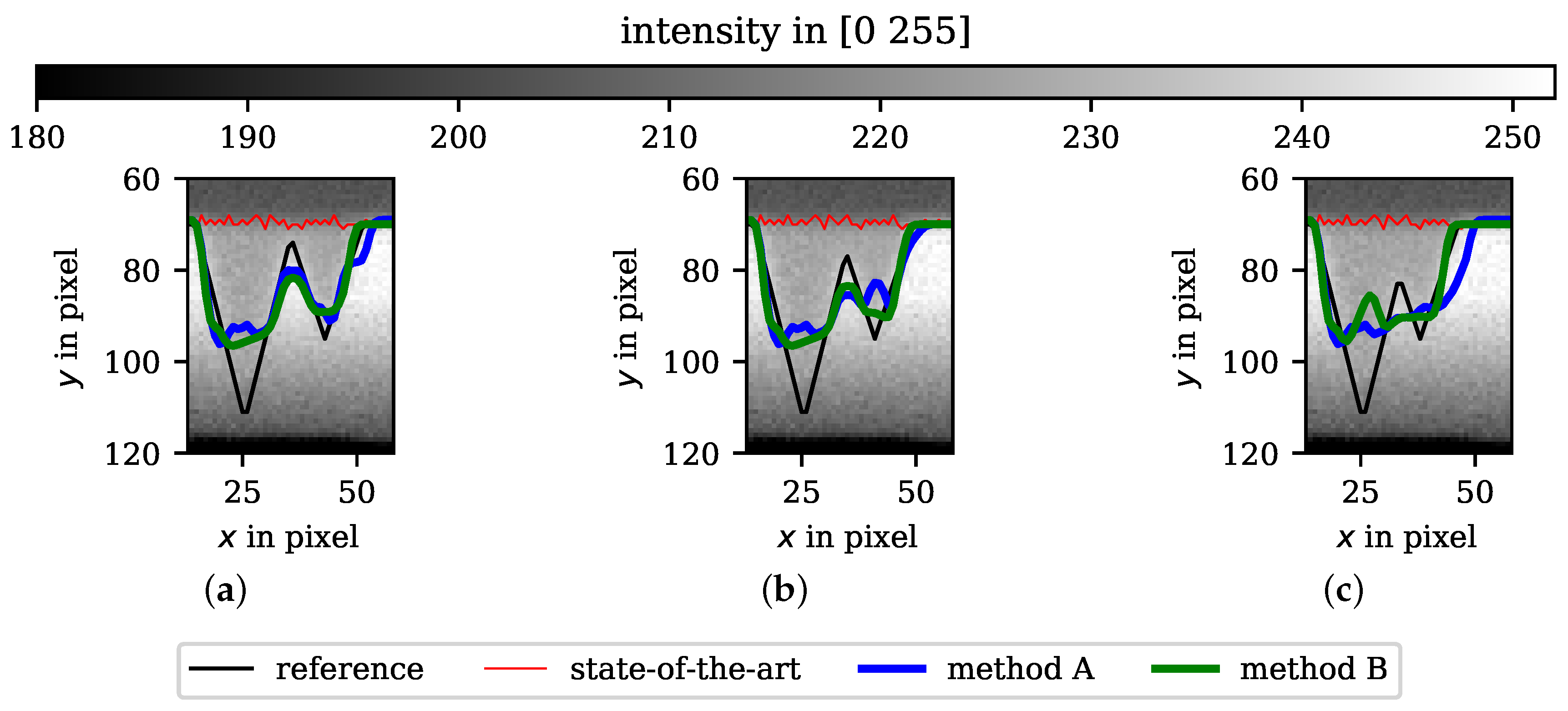
Figure 7a depicts a simulated flow visualization of a rotor blade segment with premature flow transitions triggered by a leading edge surface defect at px, developing a turbulence wedge downstream (negative y-direction) until the natural flow transition line spans along the whole segment at . Figure 7b,c shows the image section of the marked area in Figure 7a and present the results of the introduced image processing methods A (blue) and B (green) described in Section 3.2. The state-of-the-art image processing method is shown with a red line for comparison.
In contrast to the state-of-the-art method, the gradient evaluation methods A and B are able to detect the premature flow transitions and correctly locate the transition line with the exception of the area at the tip of the turbulence wedge, see Figure 7b,c. The reason for this is a low intensity area near the leading edge preventing the formation of a gradient by which the flow transition can be located. As a result, the tip of the turbulence wedge is not included in the final computed transition line, see Figure 7d. Figure 7d also depicts the true flow transition line (black) of the simulated image to be compared with the final transition lines calculated by the two gradient evaluation methods A and B. As a figure of merit for the distance between the computed and true transition lines, the mean euclidean distance is calculated as the mean of all minimum euclidean distances between each point of the computed transition line and the true transition line over both image dimension. This distance is px for method A and px for method B. The distance calculation is conducted only in the area of the turbulence wedge to increase the focus on the detection of premature flow transitions.
4.1.2. Contrast of Turbulence Wedge
The analysis of the image noise in real measurements as reference yields a standard deviation for the laminar flow regime of and the turbulent flow regime of . With the mean intensity and , the contrast to noise ratio (CNR) between the flow regimes, calculated by
is .
In order to evaluate the robustness of the introduced image processing methods for localizing premature flow transitions with respect to the magnitude of the local gradient maxima, the simulated image from Figure 7a is reconstructed with varying contrast between the turbulence wedge and the surrounding laminar flow regime. By keeping the magnitude of the image noise equal to the level measured in real measurements, this results in a reduction of the CNR between the respective surface areas. To enable a more intuitive understanding, the turbulence wedge contrast is defined relative to the contrast between the laminar and turbulent flow regime on rotor segments without premature flow transitions (). Turbulence wedges with a low intensity, see case C in Section 1.2, have a ; a contrast of represents a turbulence wedge indistinguishable from the surrounding laminar flow regime. Typically occurring values for in real measurement images are between and .
Figure 8a–c shows the same simulated flow visualization as in Figure 7 with three different relative contrast values of the turbulent wedges of , , and , respectively. The final computed flow transition line of the evaluation method A (blue) and B (green) as well as the state-of-the-art method are shown for each image. The CNR value of the three images is 163, 73, and 18, respectively. For the high contrast, see Figure 8a, methods A and B of the introduced image processing are able to locate the flow transition line with much lower uncertainties compared to the state-of-the-art method that is only able to locate individual premature flow transitions. For a contrast of , the introduced methods prove to be able to detect the turbulence wedge which remains undetected by the state-of-the-art method. For the low contrast of , the premature flow transitions remain undetected for all evaluation methods.
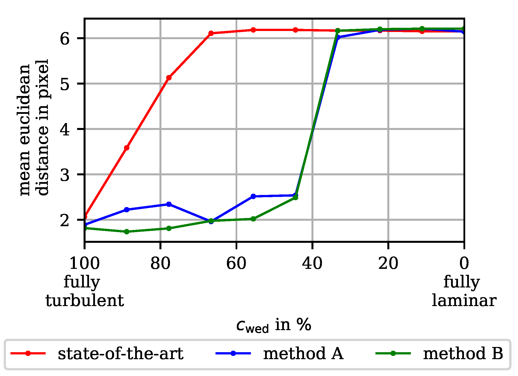
Figure 9 shows the mean euclidean distance between the true transition line and the evaluation results for 10 calculations between (fully turbulent) and (fully laminar) relative contrast between the turbulence wedge and the surrounding laminar flow regime in a simulated image similar to Figure 8. The sharp increase of the mean euclidean distance at for method A (blue) and B (green) can be explained by the use of a natural flow transition threshold. A low relative contrast of the turbulence wedge increases the local gradients at the position of the natural flow transition, see case C in Section 1.2. If these gradients are above a certain threshold, all local gradient maxima stream upwards that might represent premature flow transitions are discarded. As a consequence, the turbulence wedge is not detected. The magnitude of , below which the premature flow transitions are disregarded, can be noted by means of the sudden increase in the mean euclidean distance and is the result of the compromise between robustness and sensitivity for the image processing. Compared to the state-of-the-art image processing (red), both introduced methods are able to cope with a much lower contrast, proving to detect turbulence wedges which remain undetected by the state-of-the-art method. Additionally, for high enough contrasts, the mean euclidean distance of method A and B is lower compared to the state-of-the-art method, proving the reduced uncertainty for the transition line localization for all detected turbulence wedges.
4.1.3. Image Noise
In order to evaluate the influence of image noise on the flow transition localization, multiple simulated images similar to Figure 8 are constructed with different noise amplitudes. The relative contrast between the turbulence wedge to the surrounding laminar flow regimes is chosen as and equals the average occurring contrast analyzed in the real measurement image.
Figure 10 shows the three turbulence wedges with the image processing results. The relative noise amplitudes for the image is (a) , (b) , and (c) times the measured image noise in a real, reference image. The corresponding CNR are 496, 73, and 33, respectively. With an increasing noise amplitude and reduced CNR, all methods detect local gradient maxima caused by the image noise and not the premature flow transition and falsely interpret them as premature flow transitions. As a consequence, the mean euclidean distance between the true transition line and the evaluated transition line increases.
Figure 11 shows the result of the mean euclidean distance evaluation for a CNR of approximately 500 to 0 for a simulated image similar to Figure 10. This corresponds to a noise magnitude of a factor of approximately to the noise magnitude in real measurements. The mean euclidean distance of the state-of-the-art image processing (red) is only shown as reference and should not be focused on, as the method already fails to locate the turbulence wedge for high CNR. The course of the mean euclidean distance for the introduced image processing methods A (blue) and B (green) is increasing with reduced CNR, as the increased noise results in falsely detected premature flow transitions. Both introduced methods prove to be robust towards image noise as the mean euclidean distance does not increase considerably until the noise amplitude reaches a level 1.5 times the reference magnitude in real measurements.
4.1.4. Overlapping of Turbulence Wedges
The position of the turbulence wedges on the rotor blade depends on the location of surface defects triggering the premature flow transitions. Therefore, multiple turbulence wedges can be positioned closely to each other and overlap. In order to illustrate the capability of the introduced image processing methods to detect premature flow transitions even if the turbulence wedges are overlapping, simulated thermographic image similar to Figure 10 are created. Figure 12 shows the thermographic flow visualization with (a) two separated turbulence wedges, (b) two turbulence wedges with a medium overlap, and (c) two turbulence wedges greatly overlapping. All turbulence wedges have a relative contrast of .
The image processing methods A (blue) and B (green) are both able to cope with the overlapping of turbulence wedges and location of the flow transition line. For the test case of closely overlapping turbulence wedges, see Figure 12c, the two turbulence wedges merge into on area. This is due to the image filtering for smoothing purposes of the image processing in order to reduce the influence of image noise and increase the robustness. Nonetheless the surface area of both turbulence wedges are detected by the introduced methods. This shows that the angle of the flow transition segments is used as a priori knowledge, but not the forming of individual turbulence wedges separated from each other. The state-of-the-art method (red) is shown as a reference but is not able to detect the premature flow transitions due to the low contrast of the turbulence wedge, see Section 4.1.2.
4.2. Validation
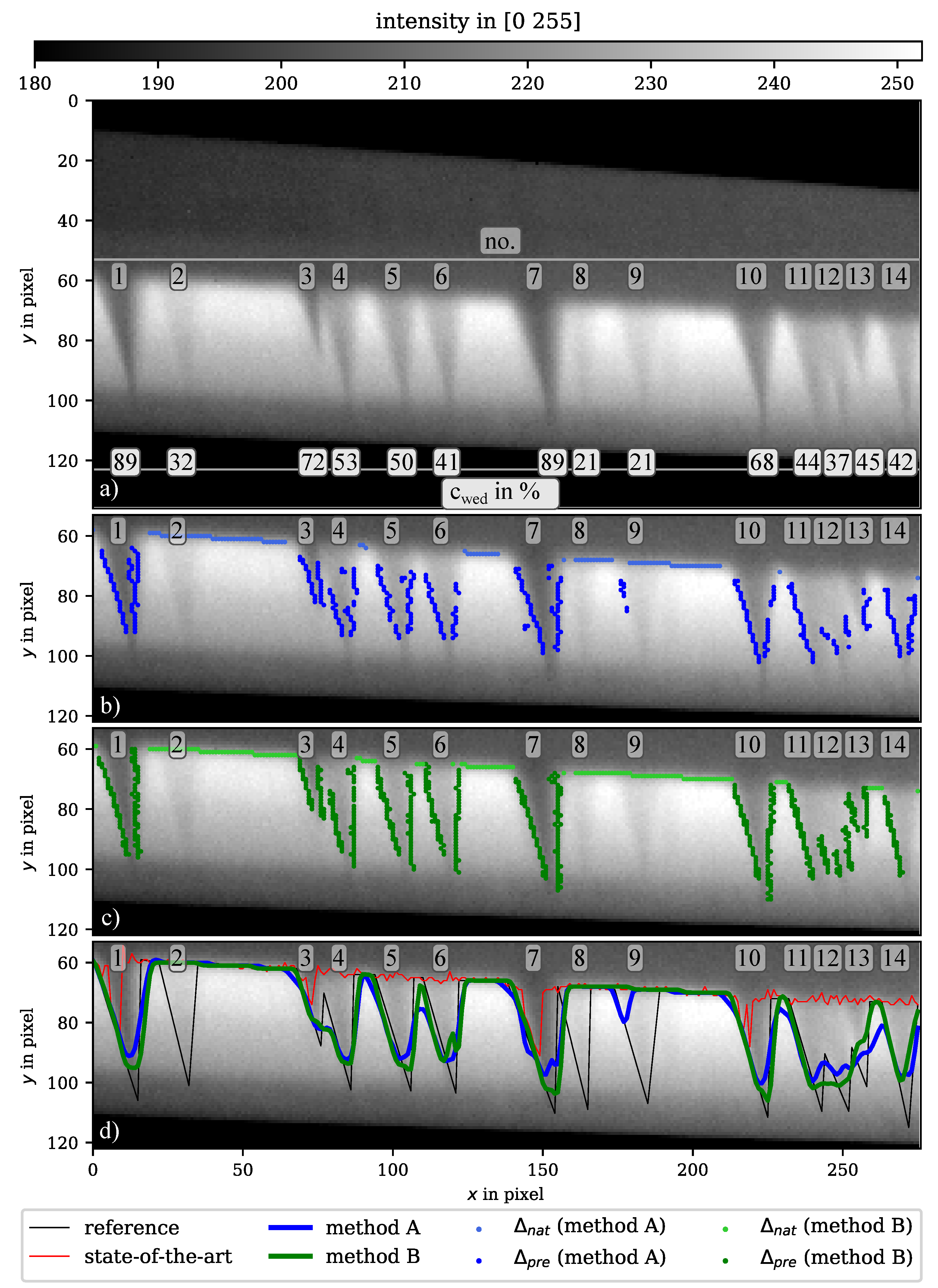
Figure 13a shows the unmodified thermographic image with multiple premature flow transitions due to surface defects, developing 14 distinct turbulence wedges of varying contrast and size. The number of each turbulence wedge and the relative contrast , defined according to Section 4.1.2, is written above and below each turbulence wedges, respectively. Figure 13b,c shows the image section of the laminar flow regime, marked in Figure 13a, with the results of the gradient evaluation for both introduced methods A (blue) and B (green). In both figures the local gradient maxima representing the natural flow transition and the ones representing the premature flow transition are differentiated by a lighter and darker coloring, respectively.
Both methods detect the natural flow transition successfully due to the strong temperature gradient in y-direction, visualized by the bright blue and bright green dots representing in Figure 13b,c, respectively. The localization of the premature flow transitions is successful for most of the turbulence wedges except turbulence wedge no. 2, 8, and 9 as their relative contrast is below the necessary threshold of , as analyzed in the verification, see Section 4.1.2. The turbulence wedges’ tips are also not detected due to no existing temperature gradients, as analyzed in Section 4.1.1.
By focusing on the turbulence wedge no. 7, methods A and B can be compared with respect to their evaluated local gradient maxima. Note hat method B is able to detect more gradients representing premature flow transitions near the tip of the turbulence wedge. As a result, the computed transition line covers a larger area, see Figure 13d.
4.2.1. Flow Transition Line
Figure 13d shows the final computed flow transition line for a comparison of the state-of-the-art (red) and the introduced image processing with both gradient evaluation methods A (blue) and B (green) as well as the manually evaluated flow transition line (black). The state-of-the-art approach is not able to locate most of the premature flow transitions, resulting in most turbulence wedges being undetected. Only in the areas of the turbulence wedges no. 1, 3, 7, and 10 some small parts of the premature flow transition line are located correctly. For the remaining image columns, the method only located the natural flow transition line. The introduced image processing methods A and B detect all 10 turbulence wedges above the critical relative contrast of . Both gradient evaluation methods were able to reduce the deviation of the located flow transition line to the actual position considerably. Therefore, the introduced image processing methods were able to locate the transition line with reduced uncertainty and maximized sensitivity with respect to the occurrences of premature flow transition, especially for low contrast turbulence wedges. The capability of the introduced image processing methods is based on assumptions on the orientation of premature transition line segments and the existence of temperature gradients at the positions of premature flow transitions. The orientations of premature flow transition line segments are almost constant throughout the image and therefore allows for an easy selection of local gradient maxima based on their direction. The existence of a high enough local gradient maxima magnitude on the other hand can vary greatly with the contrast of the turbulence wedges. Especially for low-contrast turbulence wedges, the choice of the gradient thresholds is of utmost importance. If the gradients are too low, the image processing is not capable of detecting the premature flow transitions, as noted for the turbulence wedges’ tips. Therefore, future work has to focus on alternative procedures on closing the wedges’ tips with either a model-based fitting of wedge shapes or extrapolation of the successful detected wedges’ flanks.
4.2.2. Laminar Flow Reduction
The calculated laminar flow reduction based on the introduced image processing method with both gradient evaluation methods A and B calculated by Equation (2) is listed in Table 1. The reference value was calculated by the visually inspected and manually evaluated flow transition line and amounts to , meaning that the laminar flow regime on the rotor blade surface was reduced by a quarter of its size due to surface disturbances, and therefore premature flow transitions. The for the state-of-the-art image processing method was not included as the deviation of the located transition line and reference is too high to quantify a reliable laminar flow reduction.
The absolute deviation of the between the evaluation and the reference is and for method A and B.
5. Conclusions and Outlook
An image processing method for localizing the laminar–turbulent flow transition line in thermographic images of wind turbine rotor blades in operation which is sensitive with respect to premature flow transitions was introduced. The transition line is located by evaluating local gradient maxima in the thermographic image. To achieve this, two gradient evaluation methods were introduced that use the a priori knowledge about the orientation of flow transition line segments. The first method uses this knowledge to analyze a 2D gradient field with respect to the magnitude and the direction of the gradients. The second method changes the alignment of a 1D gradient evaluation before applying a magnitude threshold. This way, both methods are able to maximize the sensitivity of the evaluation with respect to locate local gradient maxima representing premature flow transitions.
Both methods were verified on simulated images based on real measurements and proved to decrease the mean euclidean distance between the evaluated and true transition line location along the rotor blade surface. Additionally, a study of different contrasts between the wedge shaped premature transition regions with turbulent flow and the surrounding laminar flow regime, different magnitudes of image noise and the overlapping of premature transition regions were conducted. Both introduced methods proved to be robust towards the detection of premature flow transitions and are able to cope with lower contrasts and higher image noise compared to the state-of-the-art image processing. The measurement uncertainty of the localization was reduced by both introduced methods if a minimum contrast of the turbulence wedge is present.
Afterwards, a real thermographic image was used in order to validate the introduced image processing method. A visual inspection of the results showed that the number of detected turbulence wedges was increased to 11 turbulence wedges. As a comparison, the state-of-the-art image processing could not detect any of the turbulence wedges sufficiently. This allowed for a more accurate quantification of the laminar flow reduction (LFR) as the deviation of the evaluated flow transition line was reduced.
Due to non-existing local gradients at the position of premature flow transition near the leading edge of the rotor blade, the tips of turbulence wedges were not detected successfully by either image processing method. To improve the flow transition line localization, an extrapolation of the successful located turbulence wedges’ flanks could be conducted in order to close the wedge at their tips. Another possibility would be the fitting of wedge shapes form into located premature flow transitions. A detection of the premature flow transitions in regions without locale gradient maxima to be evaluated would further decrease the measurement uncertainty of the flow transition line localization.
The improved flow transition line localization enables more accurate estimation of the annual energy production loss as the laminar flow reduction due to surface defects can be quantified with reduced uncertainties. The image processing used in previous work focusing on this estimation is equal to the method this work denotes as state-of-the-art [27]. Consequently, by using the introduced methods, the transition line localization takes multiple turbulence wedges with low contrast into account that were excluded with the state-of-the-art method, thus improving the estimation of the annual energy production loss. As a result, the impact of the environment on the rotor blade surface condition and consequently the boundary layer flow can be analyzed more accurately. Additionally, a study of the correlation between turbulence wedge contrast and the origin of the triggered premature flow transition can be made in the future due to the improved localization of the turbulence wedges.
Author Contributions
D.G., M.S., and A.F.: Conceptualization, methodology, validation, formal analysis, writing—review and editing, funding acquisition. D.G.: Software, investigation, resources, data curation, writing—original draft preparation, visualization. A.F. and M.S.: Supervision, project administration. All authors have read and agreed to the published version of the manuscript.
Funding
This research was funded by Bundesministerium für Wirtschaft und Energie (BMWi) grant number 03EE3013.
Conflicts of Interest
The authors declare no conflict of interest.
Abbreviations
The following abbreviations are used in this manuscript.
| CNR | contrast to noise ratio |
| IFOV | instantaneous field of view |
| LFR | laminar flow reduction |
| method A | image processing with no image rotation and 2D gradient evaluation |
| method B | image processing with image rotation and 1D gradient evaluation |
| NETD | noise equivalent temperature difference |
| rotation angle in degrees | |
| gradient direction in degrees | |
| relative contrast of turbulence wedge in % | |
| contrast to noise ratio between area a and b in arbitrary units | |
| gradient threshold for premature flow transitions without unit | |
| gradient threshold for natural flow transitions without unit | |
| collection of premature flow transitions in pixels | |
| collection of natural flow transitions in pixels | |
| G | gradient magnitude without unit |
| gradient magnitude in direction without unit | |
| counting variable without unit | |
| mean intensity without unit | |
| relative laminar flow reduction in image column i in arbitrary units | |
| relative laminar flow reduction in arbitrary units | |
| standard deviation without unit | |
| temperature profile of image column j without unit | |
| image coordinates in pixels | |
| rotated image coordinates in pixels | |
| actual transition position in image column i in pixels | |
| natural transition position in image column i in pixels | |
| rotor blade leading edge position in image column i in pixels | |
| rotor blade trailing edge position in image column i in pixels | |
| y-coordinates of actual flow transition line in pixels | |
| y-coordinates of natural flow transition line in pixels |
References
- Schlichting, H. Boundary-Layer Theory; McGraw-Hill: Braunschweig, Germany, 1979. [Google Scholar]
- Corten, G.P.; Veldkamp, H.F. Insects can halve wind-turbine power. Nature 2001, 412, 41. [Google Scholar] [CrossRef] [PubMed]
- Dalili, N.; Edrisy, A.; Carriveau, R. A review of surface engineering issues critical to wind turbine performance. Renew. Sustain. Energy Rev. 2009, 13, 428–438. [Google Scholar] [CrossRef]
- Keegan, M.H.; Nash, D.H.; Stack, M.M. On erosion issues associated with the leading edge of wind turbine blades. J. Phys. Appl. Phys. 2013, 46, 383001. [Google Scholar] [CrossRef] [Green Version]
- Slot, H.M.; Gelinck, E.R.M.; Rentrop, C.; van der Heide, E. Leading edge erosion of coated wind turbine blades: Review of coating life models. Renew. Energy 2015, 80, 837–848. [Google Scholar] [CrossRef]
- Gaudern, N. A practical study of the aerodynamic impact of wind turbine blade leading edge erosion. J. Phys. Conf. Ser. 2014, 524, 012031. [Google Scholar] [CrossRef]
- Sagol, E.; Reggio, M.; Ilinca, A. Issues concerning roughness on wind turbine blades. Renew. Sustain. Energy Rev. 2013, 23, 514–525. [Google Scholar] [CrossRef]
- Kuester, M.S.; Brown, K.; Meyers, T.; Intaratep, N.; Borgoltz, A.; Devenport, W.J. Wind Tunnel Testing of Airfoils for Wind Turbine Applications. Wind. Eng. 2015, 39, 651–660. [Google Scholar] [CrossRef]
- Dollinger, C.; Balaresque, N.; Sorg, M.; Goch, G. Thermographic measurement method for turbulence boundary layer analysis on wind turbine airfoils. In Proceedings of the Wind Power Conference and Exhibition, Las Vegas, NV, USA, 7–8 October 2014. [Google Scholar]
- Ehrmann, R.S.; White, E.B.; Maniaci, D.C.; Chow, R.; Langel, C.M.; van Dam, C.P. Realistic Leading-Edge Roughness Effects on Airfoil Performance. Am. Inst. Aeronaut. Astronaut. 2013. [Google Scholar] [CrossRef]
- Sareen, A.; Sapre, C.A.; Selig, M.S. Effects of leading edge erosion on wind turbine blade performance. Wind Energy 2014, 17, 1531–1542. [Google Scholar] [CrossRef]
- Han, W.; Kim, J.; Kim, B. Effects of contamination and erosion at the leading edge of blade tip airfoils on the annual energy production of wind turbines. Renew. Energy 2018, 115, 817–823. [Google Scholar] [CrossRef]
- Zidane, I.F.; Saqr, K.M.; Swadener, G.; Ma, X.; Shehadeh, M.F. On the role of surface roughness in the aerodynamic performance and energy conversion of horizontal wind turbine blades: A review. Int. J. Energy Res. 2016, 40, 2054–2077. [Google Scholar] [CrossRef]
- Schaffarczyk, A.P.; Schwab, D.; Breuer, M. Experimental detection of laminar-turbulent transition on a rotating wind turbine blade in the free atmosphere. Wind Energy 2016, 20, 211–220. [Google Scholar] [CrossRef]
- Eggleston, D.M.; Starcher, K. A Comparative Study of the Aerodynamics of Several Wind Turbines Using Flow Visualization. J. Sol. Energy Eng. 1990, 112, 301–309. [Google Scholar] [CrossRef]
- Swytink-Binnema, N.; Johnson, D.A. Digital tuft analysis of stall on operational wind turbines. Wind Energy 2016, 19, 703–715. [Google Scholar] [CrossRef]
- De Luca, L.; Carlomagno, G.M.; Buresti, G. Boundary layer diagnostics by means of an infrared scanning radiometer. Exp. Fluids 1990, 9, 121–128. [Google Scholar] [CrossRef]
- Gartenberg, E.; Roberts, A.S. Airfoil transition and separation studies using an infrared imaging system. J. Aircr. 1991, 28, 225–230. [Google Scholar] [CrossRef]
- Gleichauf, D.; Dollinger, C.; Balaresque, N.; Gardner, A.D.; Sorg, M.; Fischer, A. Thermographic flow visualization by means of non-negative matrix factorization. Int. J. Heat Fluid Flow 2020, 82, 108528. [Google Scholar] [CrossRef]
- Joseph, L.A.; Borgoltz, A.; Devenport, W. Infrared thermography for detection of laminar-turbulent transition in low-speed wind tunnel testing. Exp. Fluids 2016, 57, 77. [Google Scholar] [CrossRef]
- Gartenberg, E.; Roberts, A.S. Twenty-five years of aerodynamic research with infrared imaging. J. Aircr. 1992, 29, 161–171. [Google Scholar] [CrossRef]
- Montelpare, S.; Ricci, R. A thermographic method to evaluate the local boundary layer separation phenomena on aerodynamic bodies operating at low Reynolds number. Int. J. Therm. Sci. 2004, 43, 315–329. [Google Scholar] [CrossRef]
- Dollinger, C.; Balaresque, N.; Sorg, M.; Fischer, A. IR thermographic visualization of flow separation in applications with low thermal contrast. Infrared Phys. Technol. 2018, 88, 254–264. [Google Scholar] [CrossRef]
- Traphan, D.; Herráez, I.; Meinlschmidt, P.; Schlüter, F.; Peinke, J.; Gülker, G. Remote surface damage detection on rotor blades of operating wind turbines by means of infrared thermography. Wind Energy Sci. Discuss. 2018, 3, 629–650. [Google Scholar] [CrossRef] [Green Version]
- Ye, Q.; Avallone, F.; Ragni, D.; Choudhari, M.M.; Casalino, D. Effect of Surface Roughness on Boundary Layer Transition and Far Field Noise. In Proceedings of the 25th AIAA/CEAS Aeroacoustics Conference, Delft, The Netherlands, 20–23 May 2019; Volume 2019. [Google Scholar] [CrossRef]
- Dollinger, C. Thermografische Strömungsvisualiserung an Rotorblättern Von Windenergieanlagen. Ph.D. Thesis, Universität Bremen, Bremen, Germany, 2018. [Google Scholar]
- Dollinger, C.; Balaresque, N.; Gaudern, N.; Gleichauf, D.; Sorg, M.; Fischer, A. IR thermographic flow visualization for the quantification of boundary layer flow disturbances due to the leading edge condition. Renew. Energy 2019, 138, 709–721. [Google Scholar] [CrossRef]
- Dollinger, C.; Sorg, M.; Balaresque, N.; Fischer, A. Measurement uncertainty of IR thermographic flow visualization measurements for transition detection on wind turbines in operation. Exp. Therm. Fluid Sci. 2018, 97, 279–289. [Google Scholar] [CrossRef]
- Bertalmio, M.; Bertozzi, A.L.; Sapiro, G. Navier-Stokes, Fluid Dynamics, and Image and Video Inpainting. In Proceedings of the 2001 IEEE Computer Society Conference on Computer Vision and Pattern Recognition, Kauai, HI, USA, 8–14 December 2001. [Google Scholar]
Figure 1.
Sketch of a rotor blade with a turbulent (dark) and laminar (bright) flow regime. Multiple local surface disturbances trigger premature flow transitions resulting in turbulence wedges within the laminar flow regime. Blue dashed line: Natural flow transition line if no surface disturbances would exist. Red solid line: Actual flow transition line including premature flow transitions. Three evaluation line examples are given for no premature flow transition (A), a premature flow transition at a strong turbulence wedge (B), and a premature flow transition at a soft turbulence wedge (C). The respective temperature profiles and gradients over y are shown in Figure 2.

Figure 2.
Sketch of (a) the temperature profile and (b) the temperature gradient of the three evaluation lines A, B, and C in Figure 1. The star-symbol marks the location of the actual flow transition. The flat temperature rise in the profile B with a premature flow transition results in a lower gradient compared to the profile A and therefore has a lower sensitivity with respect to the flow transition position. For the low-contrast turbulence wedge example C, the location of the flow transition does not correspond with the global but a local gradient maximum, which is lower than for a strong turbulence wedge B.

Figure 3.
Sketch of the rotation motions of the thermographic image and the evaluation line (black line) parallel to the -axis. The rotation angles and align one group of premature transition line segments perpendicular to the evaluation line, respectively. The angles between the evaluation line and the flow transition line (black dashed line) are almost perpendicular, increasing the sensitivity of the local gradient maxima localizations.

Figure 4.
Sketch of the parameter used for calculating the relative length of premature turbulent flow in column i normalized to the distance of laminar flow if no premature flow transition would occur: the distance between leading edge and natural flow transition . The laminar flow reduction (LFR) is a figure of merit for the reduction of the laminar flow regime surface area due to premature flow transitions triggered by surface defects.

Figure 5.
Experimental set-up for field measurements for the thermographic flow visualization containing an IR-camera, an optical trigger camera and the measurement unit.
Figure 5.
Experimental set-up for field measurements for the thermographic flow visualization containing an IR-camera, an optical trigger camera and the measurement unit.

Figure 6.
Flow chart of the image processing method, divided in five main parts: (1) A pre-evaluation of the thermographic image. (2) The localization of local gradient maxima. (3) Selection of gradients representing the flow transition. (4) Construction of the actual and natural flow transition line. (5) Calculation of the laminar flow reduction.
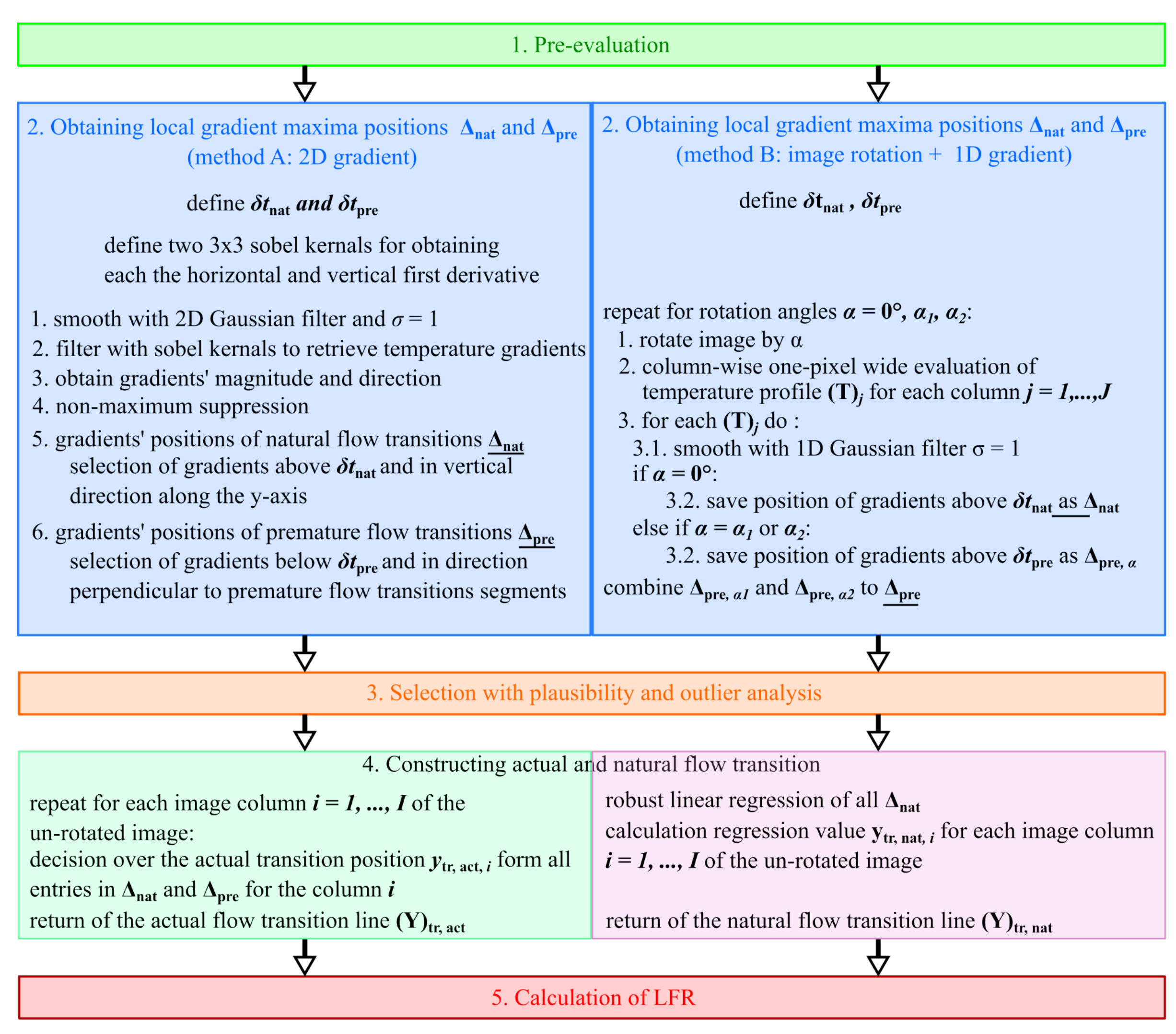
Figure 7.
Simulated thermographic flow visualization image with premature flow transitions along the flanks of a turbulence wedge. (a) Rotor blade surface section with a laminar (brighter) and turbulent (darker) flow regime. The rectangle marks the selected area shown in panels (b–d). (b,c) Evaluation of local gradient maxima for both introduced image processing methods A (blue) and B (green) and the state-of-the-art method (red). (d) True flow transition line in black as a reference as well as all image processing results.

Figure 8.
Simulated thermographic flow visualization image with premature flow transitions along the flanks of a turbulence wedge. The relative contrast between the turbulence wedge and the surrounding laminar flow regime is (a) , (b) , and (c) . In contrast to the state-of-the-art method, the introduced image processing methods A (blue) and B (green) are able to detect the turbulence wedge with a of , see panel (b). A relative contrast of is too low and results in no detected premature flow transitions for all image processing methods, and therefore the turbulence wedge remains undetected, see panel (c).
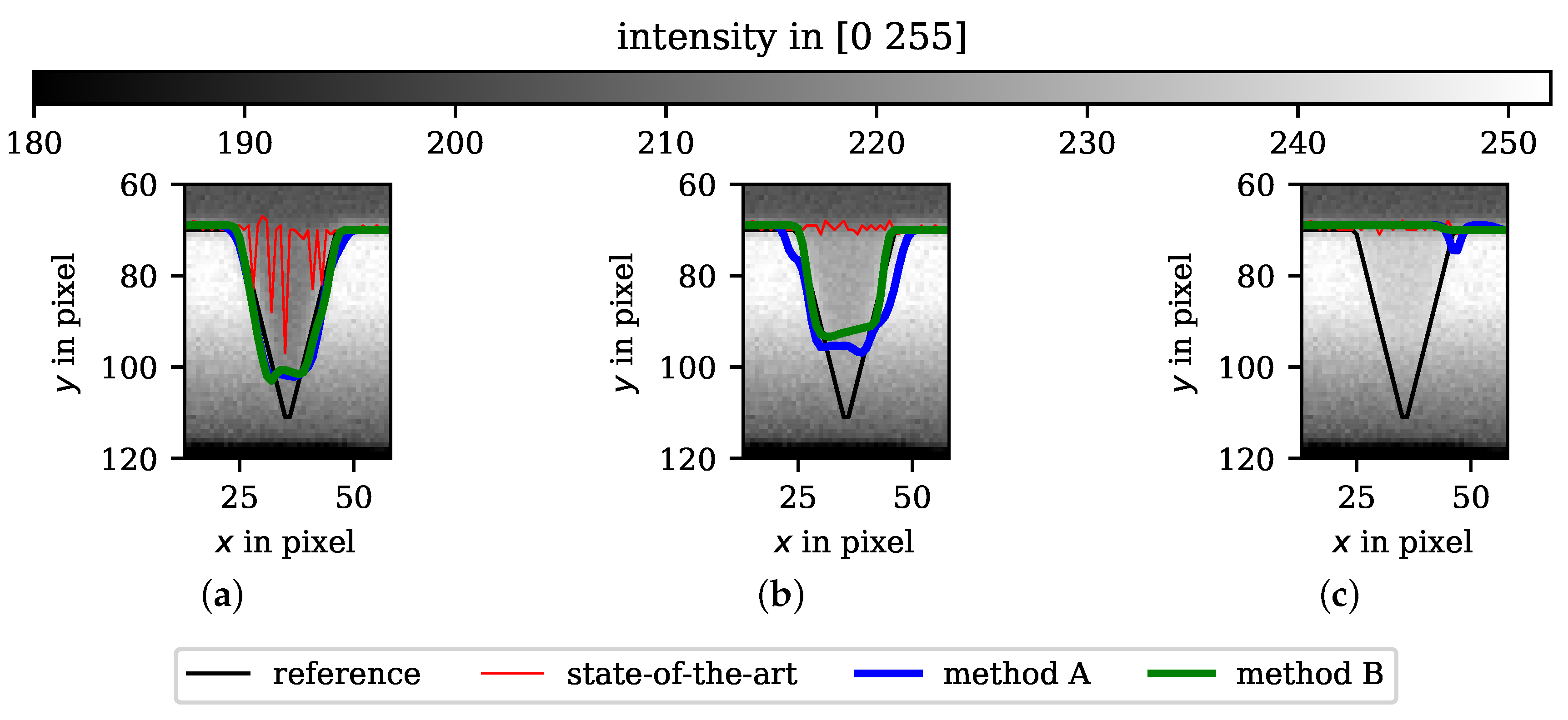
Figure 9.
Mean euclidean distance between the true transition line and the evaluated transition lines of the state-of-the-art image processing (red), method A (blue), and method B (green) over the relative contrast of the turbulence wedge from the maximum ( = fully turbulent wedge) to the minimum ( = fully laminar wedge). The introduced image processing methods A and B are able to cope with a much lower contrast (~) compared to the state-of-the-art method (~) at which the evaluation is still able to detect the turbulence wedge. This contrast limit for the detection can be noted by the sudden increase of the mean euclidean distance for lower .

Figure 10.
Simulated thermographic flow visualization image with premature flow transitions along the flanks of a turbulence wedge with a relative contrast of . The relative noise amplitude is (a) , (b) , and (c) times the measured image noise in a real, reference image. The corresponding CNR are 496, 73, and 33, respectively. Increasing noise results in more local gradient maxima falsely interpreted as premature flow transitions. The consequence is an increased uncertainty of the flow transition line for method A (blue) and B (green).

Figure 11.
Mean euclidean distance between the true and the evaluated transition lines of the state-of-the-art image processing (red), method A (blue), and method B (green) over the CNR between the turbulence wedge and the surrounding laminar flow regime. The relative contrast of the turbulence wedge is . The mean euclidean distance of method A and B increases with increasing noise but remains below the state-of-the-art method. This proves that the introduced image processing is robust towards even low CNR.

Figure 12.
Evaluated flow transition line location in a simulated thermographic flow visualization with premature flow transitions along the flanks of two turbulence wedges. The position of the two turbulence wedges is varied between (a) not-overlapping, (b) medium overlapping, and (c) greatly overlapping. The relative contrast of all turbulence wedge is . Both introduced image processing methods A (blue) and B (green) are able to cope with the overlapping of two turbulence wedges as it occurs in real measurements.

Figure 13.
Measured thermographic image for flow visualization. (a) Complete image with marked laminar flow regime area with a numbering above and relative contrast below for each turbulence wedges. (b,c) Located local temperature gradient maxima (brighter) and (darker) of both introduced gradient evaluation methods A and B in blue and green, respectively. (d) Final evaluated transition line of the state-of-the-art evaluation (red), the evaluation of methods A (blue) and method B (green), as well as the manually evaluated transition line (black) as reference.


Table 1.
Calculated laminar flow reduction compared between the manual transition line evaluation and the two introduced image processing methods.
Table 1.
Calculated laminar flow reduction compared between the manual transition line evaluation and the two introduced image processing methods.
| Method A | Method B | |
|---|---|---|
| = |
© 2020 by the authors. Licensee MDPI, Basel, Switzerland. This article is an open access article distributed under the terms and conditions of the Creative Commons Attribution (CC BY) license (http://creativecommons.org/licenses/by/4.0/).
Share and Cite
MDPI and ACS Style
Gleichauf, D.; Sorg, M.; Fischer, A. Contactless Localization of Premature Laminar–Turbulent Flow Transitions on Wind Turbine Rotor Blades in Operation. Appl. Sci. 2020, 10, 6552. https://doi.org/10.3390/app10186552
AMA Style
Gleichauf D, Sorg M, Fischer A. Contactless Localization of Premature Laminar–Turbulent Flow Transitions on Wind Turbine Rotor Blades in Operation. Applied Sciences. 2020; 10(18):6552. https://doi.org/10.3390/app10186552
Chicago/Turabian StyleGleichauf, Daniel, Michael Sorg, and Andreas Fischer. 2020. "Contactless Localization of Premature Laminar–Turbulent Flow Transitions on Wind Turbine Rotor Blades in Operation" Applied Sciences 10, no. 18: 6552. https://doi.org/10.3390/app10186552
Note that from the first issue of 2016, this journal uses article numbers instead of page numbers. See further details here.